Migrating towards Using Electric Vehicles in Campus-Proposed Methods for Fleet Optimization


1
Smart Infrastructure Research Center, Korea Research Institute for Human Settlements, 5 Gukchaegyeonguwon-ro, Sejong-si 30147, Korea
2
Department of Civil and Environmental Engineering, University of Tennessee, 311 John D. Tickle Building, Knoxville, TN 37996-2313, USA
*
Author to whom correspondence should be addressed.
Sustainability 2018, 10(2), 285; https://doi.org/10.3390/su10020285
Submission received: 28 September 2017
/
Revised: 15 January 2018
/
Accepted: 18 January 2018
/
Published: 23 January 2018
(This article belongs to the Special Issue Control and Optimization of Alternative-Energy Vehicles for Sustainable Transportation)
Abstract
:Managing a fleet efficiently to address demand within cost constraints is a challenge. Mismatched fleet size and demand can create suboptimal budget allocations and inconvenience users. To address this problem, many studies have been conducted around heterogeneous fleet optimization. That research has not included an examination of different vehicle types with travel distance constraints. This study focuses on optimizing the University of Tennessee (UT) motor pool which has a heterogeneous fleet that includes electric vehicles (EVs) with a travel distance and recharge time constraint. After assessing UT motor pool trip patterns as a case study, a queuing model was used to estimate the maximum number of each vehicle type needed to minimize the expected customer wait time to near zero. The break-even point is used for the optimization model to constrain the minimum number of years that electric vehicles should be operated under the no-subsidy assumption. The results show that the fleet has surplus vehicles. In addition to reducing the number of vehicles, total fleet costs could be minimized by using electric vehicles for all trips less than 100 miles. The models are flexible and can be applied and help fleet managers make decisions about fleet size and EV adoption.
1. Introduction
Managing a fleet efficiently to address demand within cost constraints is a challenge. A fleet management program balances many objectives, including driver management, speed management, fuel management, route management, fleet size, and composition management. If those objectives are not balanced, users may be inconvenienced and total fleet costs could be suboptimal. This study examines fleet size and composition management, with a focus on the role of electric vehicles (EVs) in corporate passenger car fleets. Several earlier studies have examined fleet size and composition management [1,2,3,4,5], but none have addressed the unique operational characteristics of EVs in fleet optimization.
Recently, EVs have emerged as an alternative fuel vehicle that can address many sustainability challenges. With low emissions and lower operating costs (fuel and maintenance) than conventional vehicles (CVs), they are becoming more popular in commercial use [6]. This is despite the vehicles’ significantly different performance characteristics and fixed costs, such as purchase price, depreciation, refueling infrastructure, and registration fees. An EV’s purchase price is higher than a CV’s purchase price, but this can be balanced by variable costs, like fuel, insurance, and maintenance costs. An EV’s variable costs are significantly lower than a CV’s. Beyond costs, EVs’ commercial success is impacted by two additional characteristics: their short driving distance and long refueling (recharging) time. EVs need to be driven often for the fuel cost savings to overcome the high fixed costs. Range and recharging time constrain an EV owner’s ability to maximize EV use and economic performance.
Vehicle fleets offer a unique opportunity to manage supply and demand by assigning the appropriate vehicle technology (CV or EV) for each trip. Despite that, most vehicle fleets currently rely on gasoline internal combustion engine vehicles, CVs [7]. However, EVs could easily be integrated into existing fleets. First, fleets usually have centralized parking and dispatch locations that could readily incorporate an EV charging infrastructure. Secondly, with customer’s frequent short trips, EVs could have high utilization rates. Third, with known trip distance and duration, managers can appropriately match vehicle type to individual trips.
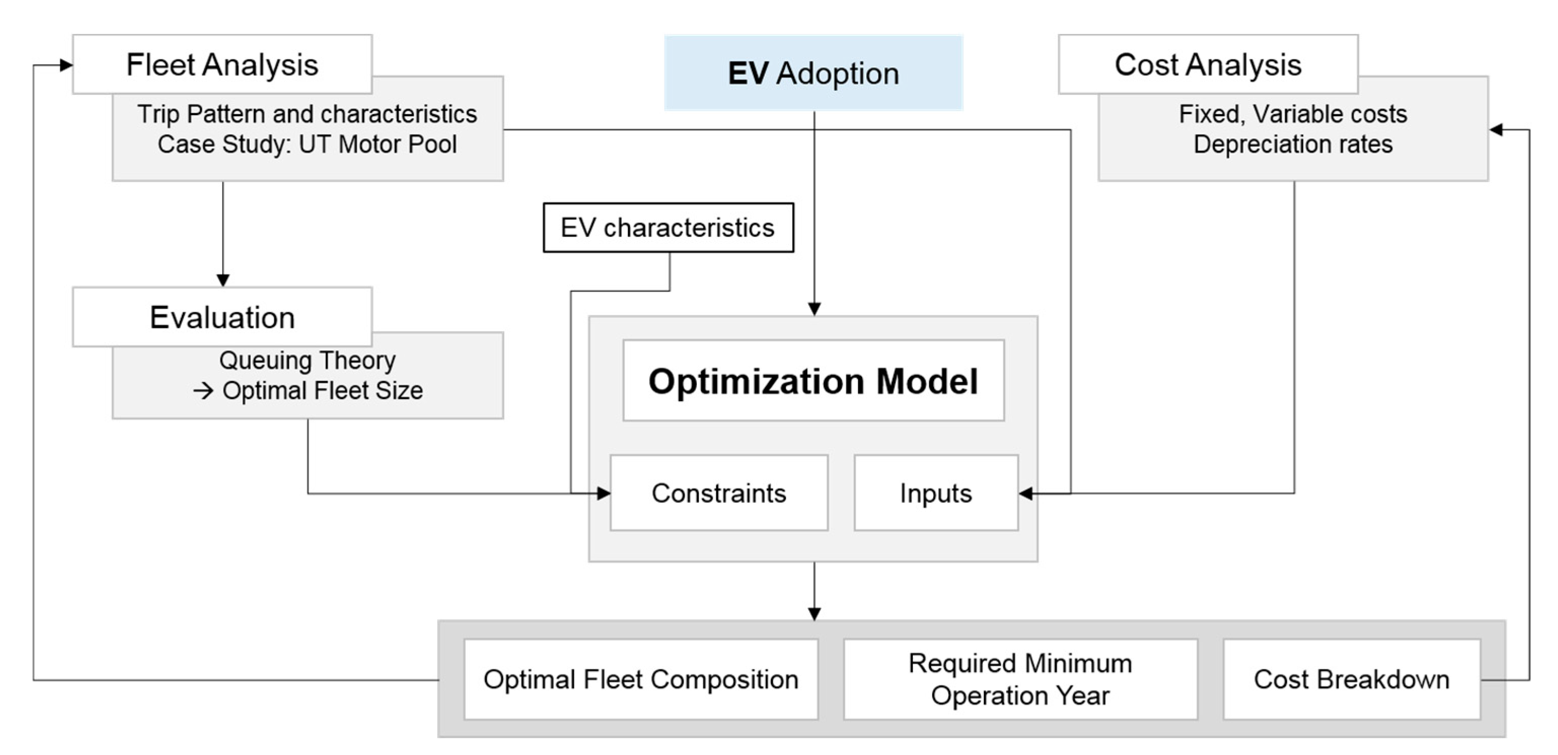
This paper develops an optimization framework for corporate fleet adoption of EVs, this includes developing a model for overall fleet size and the appropriate mix of EVs and CVs. The paper focuses on the University of Tennessee (UT) motor pool, which is located to Knoxville, Tennessee. The UT motor pool serves the transportation needs of faculty, staff, and students conducting official business. This study applies fleet optimization methods to investigate the trip patterns of the UT motor pool and finds how many of those trips are EV-compatible. Optimized fleet size, compositions, and required operating years are the objective values with cost constraints in the optimization model. Figure 1 illustrates the methodology flowchart of this paper.
This will help manage the fleet efficiently with a minimum total cost and greater demand satisfaction. The rest of this paper is organized as follows: in Section 2, we will review previous works; in Section 3 and Section 4, we will describe current fleet and its usage and estimate cost for each vehicle type; in Section 5, we will develop the model how to optimize fleet size and composition; and, finally, results and conclusion of this paper will be presented in Section 6 and Section 7.
2. Literature Review
2.1. Electric Vehicles
The transportation sector has developed plug-in battery EVs and other technologies in recognition of the importance of fuel consumption and energy security, economic efficiency, health concerns, and environmental impacts [8]. EVs (defined as battery EVs here) rely solely on battery power charged through a charging station. Balancing expensive and heavy battery capacity requirements with expected range usually results in commercial EVs with lower driving range than an equivalent CV [9].
EVs have existed for more than 150 years [10]. Due to the production efficiencies and easily available, cheap fossil fuel, CVs became widespread through the 20th century. In recent decades, battery technology improvements have allowed for improved EV designs. The industry has developed more energy-efficient and less-polluting EVs [10]. Using electricity and without tailpipe emissions, EVs can help reduce operating costs and fuel consumption [11]. EVs’ popularity can be attributed to its potential for reducing a country’s dependence on imported petroleum and its greenhouse gas (GHG) emissions [12]. This GHG reduction holds even when balancing EVs increased electric consumption that causes increased pollution from electricity generating sources [6]. Thus, recent commercialized EVs have been relatively successful with markets in the United States, Europe, and China where a new energy vehicle policy subsidizes EV deployment.
Since costs, driving range, fuel efficiency, vehicle gross weight, and other factors differ from EVs to CVs, fleets must precisely determine its vehicles’ needed specifications and characteristics. Even though the EVs’ purchase price is higher than that of gasoline or diesel vehicles, other variable costs, like fuel and maintenance, and when coupled with purchase subsidies, the registration with incentives, insurance, maintenance, repairs, and the energy price of EVs are lower than those of CVs [13,14].
This study introduces and analyzes one commercialized EV, the Nissan Leaf, because of its publically-available specification and performance information. The Nissan Leaf has an 80 kW AC synchronous electric motor, a 24 kWh lithium-ion battery, a 3.3 kW onboard charger, and a battery heater. The Environmental Protection Agency (EPA) LA-4 city cycle laboratory tests determined it has a driving range of up to 100 miles. Based upon EPA five-cycle tests, using varying driving conditions and climate controls, the EPA has rated the Nissan LEAF at a driving range of 73 miles. EPA MPG equivalent is 106 (city) and 92 (hwy) miles [15]. This study assumes that EV can drive up to 100 miles.
2.2. EV Benefits Compared to CV
In general, CVs contribute to local air pollution, noise pollution, water pollution, and other pollution [16]. Air pollution may cause reduced visibility, crop losses, material damage, forest damage, climate change, and human health impacts [17]. CVs emit many kinds of exhaust pollutants such as particulates, hydrocarbons, nitrogen oxides (NOx), carbon monoxide (CO), carbon dioxide (CO2), and other pollutants. The emissions can either affect the environment directly through diminished air quality and climate change or be precursors to species of concern, which are formed in the atmosphere. The former includes carbon monoxide (CO), and the latter includes volatile organic compounds (VOCs) and nitrogen oxides (NOx) which are precursors to the photochemical formation of ozone and PM [18]. Diesel vehicles have different emission characteristics than gasoline vehicles, e.g., NOx emission levels are higher for diesel vehicles [19].
Older vehicles without advanced pollution control technology cause a significant amount of urban emissions. Some argue for an automobile replacement policy, where old cars need to be replaced by new ones to prevent continuous use of inefficient and higher-polluting vehicles. The retirement program sometimes incentivizes owners of older vehicles to replace old vehicles earlier [20]. Kim et al. [21] suggest that vehicle retirement should be decided by economic factors, such as repair cost, market price, and scrap price of a used vehicle.
Previous research [7] concludes that the EVs can reduce 38–41% of GHG emissions compared to the CVs and 7–12% of the emissions compared to traditional hybrids. They find that the EV battery, especially lithium-ion battery material and production, accounts for 2–5% of an EV’s life cycle GHG emissions. They also point out the importance of using electricity for energy which influences GHG emissions.
Emission factors for EVs are very sensitive to the time of recharging, the source of electricity, and the region an EV is charged [22]. Coal (38%) has the largest share as the source of electricity, followed by renewables (20%), nuclear (17%), natural gas (16%), and oil (9%). Previous research expected the electricity production will be almost double by 2020. As more natural gas and nuclear power plants replace older coal power plants, this emission issue should improve [23].
2.3. Fleet Optimization Models
This paper builds on previous research to study how to utilize EVs in vehicle fleets; it develops a model based on fleet size and composition. The vehicle routing problem (VRP) serves as a precursor to the fleet optimization model. Proposed by Dantzig and Ramser in 1959, the VRP is a combinatorial optimization and integer programming approach seeking to service a number of customers with a fleet of vehicles [24]. Since its inception, numerous studies have used and developed the VRP. With several kinds of VRP, this study divides them into two categories: capacitated vehicle routing problem (CVRP) [24,25,26,27,28,29,30,31,32,33] and capacitated arc routing problem (CARP) that improves local search procedures [34].
Some have focused on heterogeneous mixed fleet optimization by narrowing down from VRP and dispatch models. Several studies [35,36,37,38,39,40] have examined the heterogeneous VRP (HVRP). In the applications of HVRP, they tried to minimize total cost by dispatching each vehicle type, defined by its capacity, a fixed cost, a distance unit, and availability.
Company fleets must decide whether to own fleet vehicles or rent them. Etezadi and Beasley [1] found that optimal fleet composition for a central depot has to supply a specific number of customers. That study developed a model that optimized the number of owned and rented vehicles to minimize total costs based on distance travelled:
- = Fixed cost associated with owning a vehicle of type j for T periods.
- = Fixed cost associated with hiring a vehicle a vehicle of type j for one period.
- = Variable cost of an owned vehicle of type j.
- = Variable cost of a hired vehicle of type j.
- . = Number of owned vehicles of type j.
- = Number of hired vehicles of type j in period t.
- = Distance travelled by owned vehicle of type j in period t.
- = Distance travelled by hired vehicle of type j in period t.
Other research was performed with six different size vehicles to optimize the size and composition. The aim of the linear model is to maximize profit and minimize total costs. The vehicle class is constrained by material and volume shipped. The developed model is shown in Equation (2) [2]:
- F = Fixed cost/day of a company-owned vehicle.
- V = Variable cost/day of a company-owned vehicle.
- H = Hiring cost/vehicle per day.
- Y = Number of working days in a year.
- N = Number of vehicles in the fleet.
- = Number of loads carried by company vehicles on days when demand is .
- = Number of loads carried by hired vehicles on days when demand is .
If the fleet is too small and cannot meet the demand, then many additional vehicles should be rented, at additional cost. To achieve the optimal fleet size, the cost to be minimized can be categorized into fixed and variable costs during the total life cycle. A novel algorithm combines dynamic programming and the golden section method to determine optimal fleet composition [3]:
- M = Number of vehicle types.
- N = Number of periods in the time horizon.
- = Fixed cost per period of a type-i vehicle.
- = Variable cost per period of a type-i vehicle.
- = Hiring cost per period of a type-i vehicle.
- = Probability that k type-i vehicles will be required during period j.
- = Maximum number of type-i vehicles required during a single period.
- = Maximum fleet size.
Previous research determined the optimal fleet size and mix for paratransit service. It shows that fleets should not only meet diverse travel needs and seating requirements of their clients, but also the decisions on how many vehicles and what types of vehicles to operate are made by managers on an ad hoc basis without much systematic analysis. The research approaches the optimization problem from the perspective of service efficiency with cost-effectiveness. Another research proposed a heuristic procedure which can be used in paratransit companies’ specific operating conditions and environments [4].
The model to optimize buy, operate, and sell policies for fleets of bus transit vehicles was developed. The model below minimizes the total discounted cost over L years which is equal to the purchase price minus reward from selling plus the cost of operating the buses [5]:
- L = Length of planning horizon in years.
- = Cost of acquiring a new bus in year i.
- = Number of new buses acquired at the beginning of year i.
- = Number of buses j years old operated during year i.
- = Number of route kilometers travelled by a bus j years old in year i.
- = Cost of operating a bus j years old in year i for kilometers (for discounting purposes, operating costs incurred during the year are treated as occurring at the beginning of the year).
Previous research also developed an optimization model that minimizes life cycle cost, petroleum consumption, and GHG emissions for conventional, hybrid, and plug-in hybrid vehicles under several scenarios. They concluded that high battery costs, low gas prices, and high electricity prices drastically reduced the financial viability of plug-in EVs [11].
There have been two studies for the University of Tennessee Motor pool fleet. Even though the data and information are old, these studies show the UT motor pool’s history. Early research in 1980 found that the UT motor pool’s vehicle request rates were time-dependent and non-stationary Poisson processes. Over 85% of the trips were five days or less. Additionally, the research performed regression analysis for check out duration and distance travelled. It shows a strong linear relationship with R2 = 0.92 (total trip mileage by length of trip). Service level and fleet utilization metrics were used to assess the motor pool’s service capability [41]. A different study pointed out that increasing the fleet reduces the number of unsatisfied requests, but increases the fixed investment in the motor pool. Additionally, they found that the peak for checking out vehicles is early in the week and that the demand decreases later in the week. The check-out duration followed an exponential distribution [42].
3. Fleet Description and Usage
The UT motor pool was set up in the early 1950s and stayed relatively small in scale for over a decade. In the 1960s the University experienced a sharp enrollment increase and requests for dispatch vehicles grew rapidly. Thus, a large number of vehicles were added to the fleet to satisfy the increasing demand [41]. Over the years many procedures have been implemented to maintain UT motor pool vehicles. Users are encouraged to use an on-site fueling station or a fleet fueling card at participating gas stations. The vehicles are maintained and repaired in-house except in cases of severe damage when the vehicles are serviced outside. Any vehicles older than three years or that have traveled 80,000 miles, whichever is first, are sold through public auctions each spring.
This study examines data collected between 14 March 2011 and 20 February 2012. The fleet consisted of 95 mid-size gasoline sedans that made a total of 1937 trips. The sedans were 2008–2011 Dodge Avengers and 2011 Ford Fusions. The rated fuel economies (averaged over four model years) ranged from 20–22 miles per gallon (mpg) for city and 28.5–30 mpg for highway driving. Since only mid-size sedans can be potentially replaced by EVs, such as the Nissan Leaf and Chevrolet Volt, only those fleet data were analyzed.
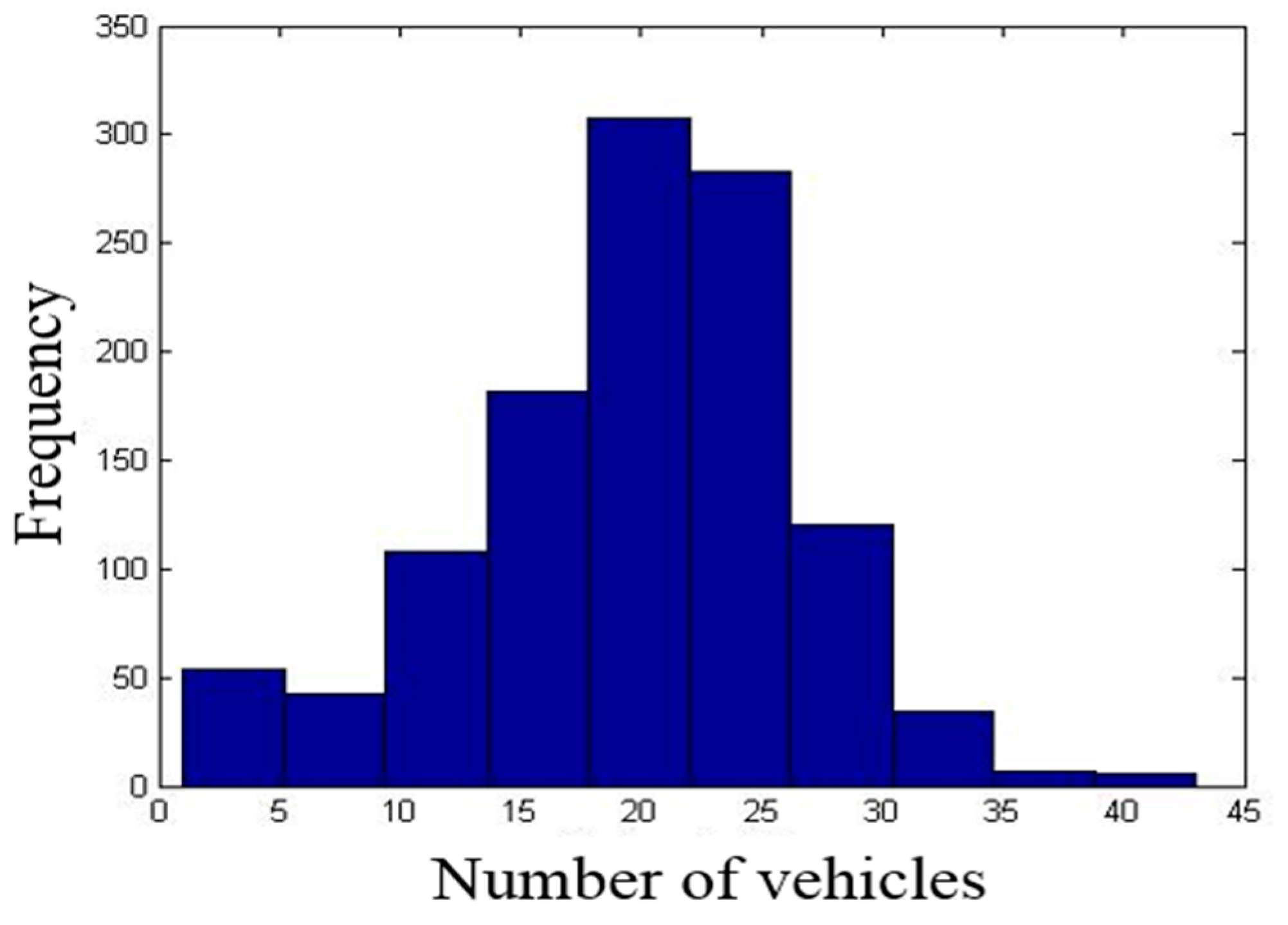
To assess the trip patterns of the UT motor pool vehicles, this study analyzed the times at which the vehicles were checked out, the distance traveled, and the destinations from the given data. The median value of checkout duration and distance traveled are 70 h (three days) and 409 miles, respectively. Around 40% of the total trips are local, meaning that the destinations were in counties bordering the UT campus in Knoxville. The destinations of 79% of the trips are within the state of Tennessee. The longer duration of checkout times reflects overnight or weekend checkouts. Figure 2 shows the frequency of the number of vehicles checked out at a given time. The most frequent number of simultaneously checked out vehicles is 43 and the average is 20–25 vehicles. This will be used to evaluate the model suggested in this paper. About 96% of demand is met by 30 vehicles.
4. Cost Assumption
All costs are included as variables, since different fleets have different rules. For example, the University of Tennessee has no federal incentives, state incentives, taxes, or registration fees. However, the developed model must be a general cost model that can apply to all fleets.
4.1. Fixed Costs
Fixed costs are the expenses that do not change as a function of the activity within the relevant period. This study includes MSRP (manufacturer’s suggested retail price), which is the list price or recommended retail price of the vehicle. The MSRP for the Dodge Avenger, which is used in the UT motor pool, and the Chevrolet Volt are $19,900 and $34,095, respectively. In the state of Tennessee, a 7% sales tax makes the final prices $21,293 and $36,482, respectively. The sales tax rates vary based on where the vehicles are registered. An additional factor for cost is an incentive that the Tennessee Department of Revenue offers, a rebate of $2500 on the first 1000 qualified plug-in EVs (PEV) purchased at Tennessee at EV dealerships [43].
4.2. Variable Costs
Variable costs are expenses that may change by time or use rates. Maintenance costs include regular drivetrain maintenance, repairs and tires, insurance costs, fuel costs, and registration. Every cost can be calculated by using NPV (net present value) which is defined as the sum of the present values of the individual cash flows of the same entity.
For the calculation of fuel costs, this research assumes the retail gasoline price is $3.25/gallon. It costs $0.13 per mile using the average of EPA mileage estimates, 25 MPG (21 City/29 Hwy). For example, when a Dodge Avenger travels 20,000 miles per year, the fuel cost is $2600 per year. A Chevrolet Volt can drive around 3 miles per kWh of electricity. This research assumes the electricity price is $0.1/kWh and costs $0.03 per mile. Thus, when a Chevrolet Volt travels 20,000 miles annually, the fuel cost is $667 per year (about 25% of the Dodge Avenger’s costs).
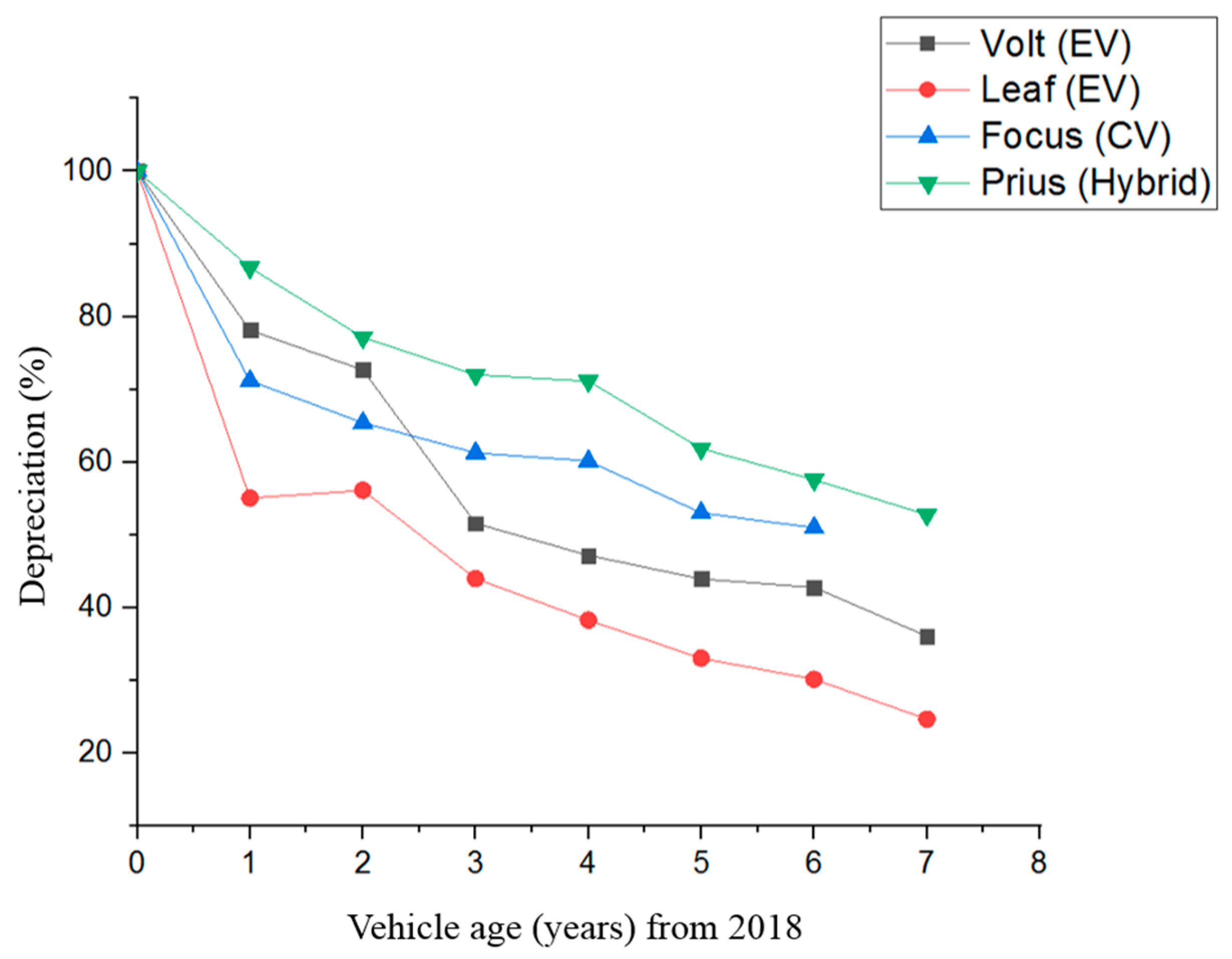
The depreciation rates by vehicle age and model are shown in Figure 3. Since the Chevrolet Volt and the Ford Focus EV (both launched in 2017) do not have a long history, four vehicles—the Chevrolet Volt (EV), the Nissan Leaf (EV), the Ford Focus (CV), the Toyota Prius (Hybrid)—were compared. The Ford Focus represents US-manufactured vehicles and the Toyota Prius represents hybrid vehicles. As expected, the depreciation rate for a hybrid vehicle is lower than that of gasoline vehicles [44]. EV models which have been more than three years after purchasing shows greater depreciation than depreciation rates of CV and hybrid vehicles, perhaps because of concern about battery lifespan and lower performance.
4.3. Break-Even Point
Since an EV’s fixed costs, such as vehicle purchase, tax, and registration, are higher than those of CVs, the break-even point (BEP) is important. This is the point at which expenses and revenue are equal so there is no net loss or gain. At that point an owner has “broken-even”. In this study, the BEP is set as the minimum time or mileage required before an EV can be resold. The EVs’ total costs become lower than the costs of the CVs after this point.
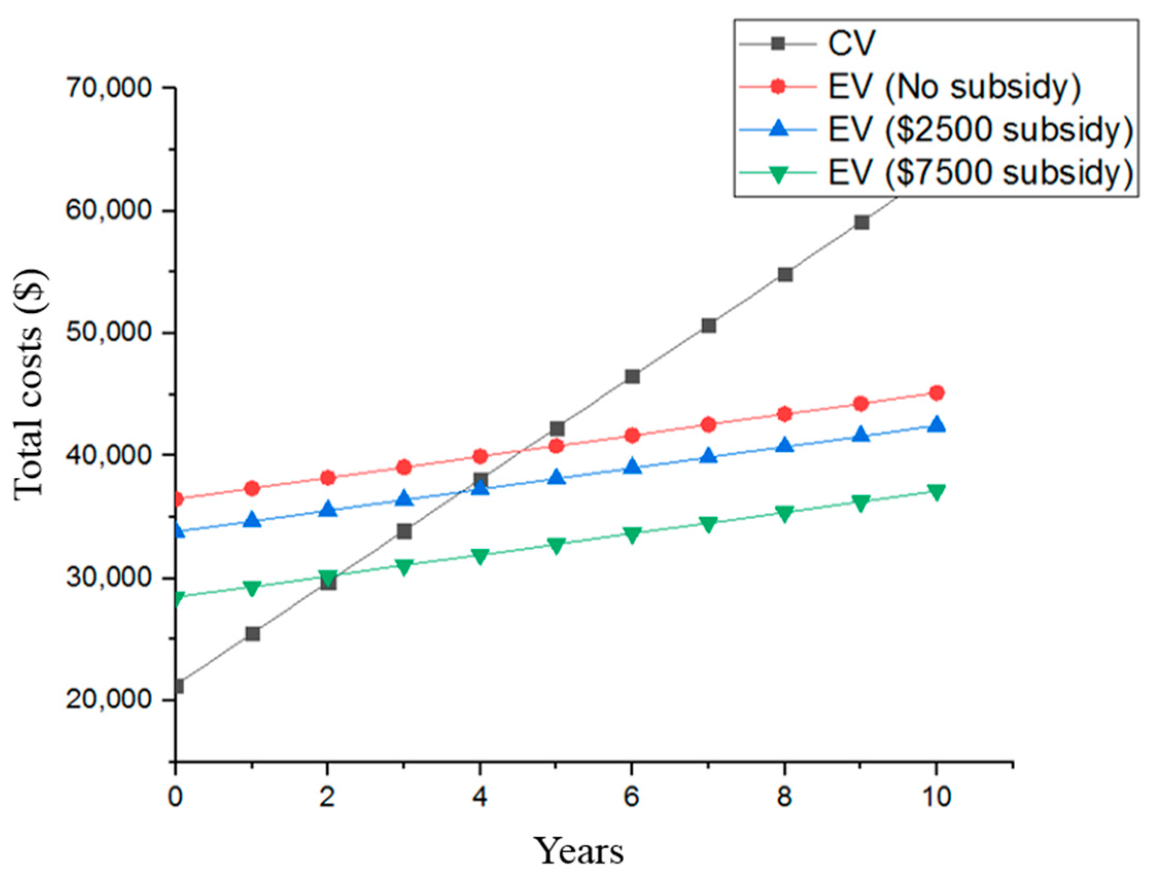
Table 1 shows the break-even point for a Chevrolet Volt and a Dodge Avenger. This assumes the cars travel 20,000 miles per year and operate for 10 years while gasoline remains $3.25/gallon and electricity is $0.1/kWh. The EV break-even points (points of contact in Figure 4) range from two years to 4.5 years with different scenarios. The break-even point will be used for optimization model to set up a constraint of the minimum number of years that EVs should be operated under the no-subsidy assumption.
5. EV Fleet Size and Composition Optimization
5.1. Fleet Size Optimization
This study utilizes a queuing model to determine the optimized fleet size based on the number of trips and trip durations to meet 100% of the demand. This study assumes that the motor pool satisfies demands and makes the probability an arriving customer has to wait near zero. For fleet composition, this study extends that analysis to access the potential for EV s in the fleet. A multiple-channel queuing model is appropriate to estimate the probability under the assumption that one vehicle plays a role as a server.
According to the data collection, a total of 1936 trips were made in 344 days. Each weekday averaged 7.9 trips. However, it is not easy to determine the number of vehicles that the motor pool needs based solely on the number of daily trips. Many other factors are important, for example the duration of checkout (particularly for multi-day use). Figure 5 illustrates the simulation flow.
This study assumes that the distribution of the arrival rate of customers is Poisson and the service time follows the exponential distribution [45]. As a multiple channel queuing model, the aim is to make the probability that an arriving customer has to wait near zero.
5.2. Fleet Composition Optimization
In this section, the total fleet size is set at fleet size (as estimated in the previous section). Assuming that the fleet may adopt EVs, what is the optimal fleet composition? To estimate what portion of CVs can be replaced by EVs (with a constraint maximum of seven EVs), the model should be optimized while minimizing total cost. Then, the model is:
5.2.1. Nomenclature
| Decision variables | |
| The number of k-type vehicle | |
| The estimated life for k-type vehicles | |
| Fixed costs | |
| The purchase price of k-type vehicle | |
| The incentive of k-type vehicle | |
| The vehicle purchase tax rate of k-type vehicle | |
| Variable costs | |
| The number of k-type vehicle in year i | |
| The travel mileage of k-type vehicle in year i | |
| The insurance costs per year of k-type vehicles in year i | |
| The maintenance costs per mile of k-type vehicles in year i | |
| The fuel costs per mile of k-type vehicle in year i | |
| The annual registration fee of k-type vehicle in year i | |
| Resale value | |
| The number of k-type sold vehicle in year i | |
| The resale value of k-type vehicles in year i | |
| R | The break-even point |
5.2.2. Optimization Model
Subject to:
The objective function (5) minimizes the total costs associated with fixed costs, variable costs, and resale value with discounted cash flows. Since the UT motor pool fleet is a self-insured fleet, this study assumes that the average insurance rate reflects expected losses. The constraints of Equations (6) and (7) require a non-negative and integer solution for all decision variables.
The constraints given in Equations (8)–(11) are the number of vehicles’ constraints. The constraint given by Equation (8) enforces the total number of k-type vehicles in year i could not exceed the total number of vehicles in year i. The constraint given by Equation (9) ensures that the total number of k-type vehicles in year i should be equal to the gap between the number of purchased and sold k-type vehicles in year i. The constraint given by Equation (10) ensures that the fleet cannot sell a vehicle that is less than one year old. The constraint given by Equation (11) assures that the number of EVs could not exceed the value attained in the queuing analysis presented above, which assures full availability of the fleet.
The constraints given in Equations (12) and (13) are cost constraints. The constraint given by Equation (12) limits total spending in i year so it will not exceed the fleet budget. The constraint given by Equation (13) enforces that total annual maintenance costs should not exceed the resale value. Fuel costs are calculated by using fuel efficiency such as mile per gallon and mile per kWh and average fuel price per unit (gallon or kWh).
The constraint given by Equation (14) enforces that the minimum estimated life for k-type vehicles in year i should be longer than the break-even year, assuring that the increased capital cost of EVs are recovered in fuel and maintenance savings before resale.
6. Results
6.1. Optimized Fleet Size
In this paper the queuing model helps determine constraints in the optimization model. Together they can determine effective fleet size and help plan EV adoption. Figure 6 indicates how long a single arrival will have to wait and shows that as the number of vehicles increases, the probability goes down. For example, if the fleet only has 10 vehicles, there is nearly 100% probability that at least one customer will have to wait. The number of vehicles assure near zero expected waiting delay is 51 from the queuing model. The average number of customers, which is the average number of vehicles that are checked out during peak times, is 27.7; and the average time a customer spends in the system is 3.5 days according to the equations in queuing model. The number of vehicles that are calculated by the queuing model looks reasonable compared with the number of vehicles that were checked out simultaneously and the considerations of vehicles’ maintenance and repair time.
This study also uses the queuing model for trips of less than 100 miles, which are suitable to be replaced by EVs. The result indicates that seven CVs can be replaced by EVs to maintain the probability that an arriving customer has to wait near 0%. This means the users who travel less than 100 miles will not need to wait to use EVs when the fleet has seven EVs. If the number of EVs is more than the estimated number, the fleet has redundant EVs that cannot meet the demand requiring a CV.
A related question is whether 44 CVs can satisfy all the other trips (not including those less than 100 miles that can use an EV). The probability that an arriving customer has to wait is near 0%, and the given numbers of EVs and CVs used as constraints from the queuing model are well estimated. Therefore, this study sets the maximum number of EVs at seven and the maximum fleet size at 51 (44 CVs) for the optimization model. With these constraints, the optimization model minimizes total costs.
6.2. Optimized Fleet Composition
Along with constraints about the maximum fleet size for each vehicle type, minimum estimated of time was also considered. As many studies set up the constraint to ensure that the fleet cannot sell a vehicle that is less than one year old, this study set up a constraint to enforce not selling EVs before it approaches the BEP. This aims to ensure that the fleet should own EVs which have higher fixed costs, such as purchase price, and lower variable costs, including fuel, maintenance costs, and depreciation for longer than BEP before resale.
Average annual total mileages estimated by the model appear reasonable compared with real data and the sum of total mileage satisfies the total fleet mileage demands. The total cost of ownership would be minimized with the estimated values in Table 2, which means that the fleet can be operated with a minimized budget when seven EVs and 44 CVs are operated for 4.5 and three years, respectively. The optimization results show that all trips less than 100 miles can be replaced by EVs with minimum total costs and those EVs should be operated for at least 4.5 years, which is later than the break-even point. It is important to note that this requires precise dispatching. It is possible that dispatching CVs for short trips will leave the EVs unable to meet demands for long trips under peak demand scenarios.
6.3. Detailed Breakdown Costs
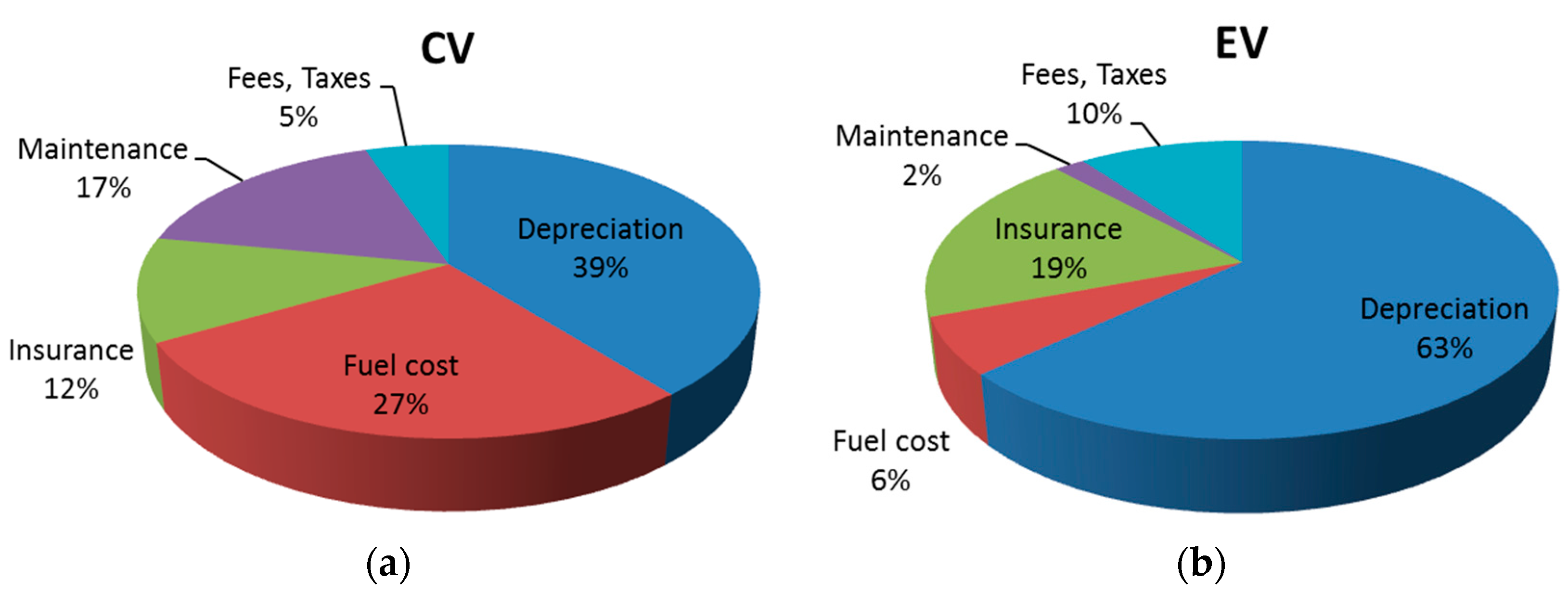
The detailed breakdown by year is shown as Figure 7. It shows that even though the EV depreciation rate is lower than CV depreciation, depreciation costs account for the largest portion of EV’s average total costs per year because of the high purchase price and low fuel and maintenance costs. It also shows the differences for maintenance and fuel costs. Fuel and maintenance costs for a CV account for 27% and 17%, respectively. On the other hand, for an EV they account for only 6% and 2% for EV. This indicates that fuel price and efficiency are the most significant factors for a CV, while a subsidy incentive to lower the high purchase price is the most significant factor to promote EV usage.
6.4. Sensitivity Analysis
We now examine the sensitivity analysis for the change of years that need to be operated. EVs need to be operated a minimum range of 5 to 10 years, while CVs have a minimum range of three to five years. That is, EVs and CVs should be operated for at least five and three years, respectively. An EV can be operated up to 10 years and a CV may be used up to five years to satisfy the minimum total costs condition.
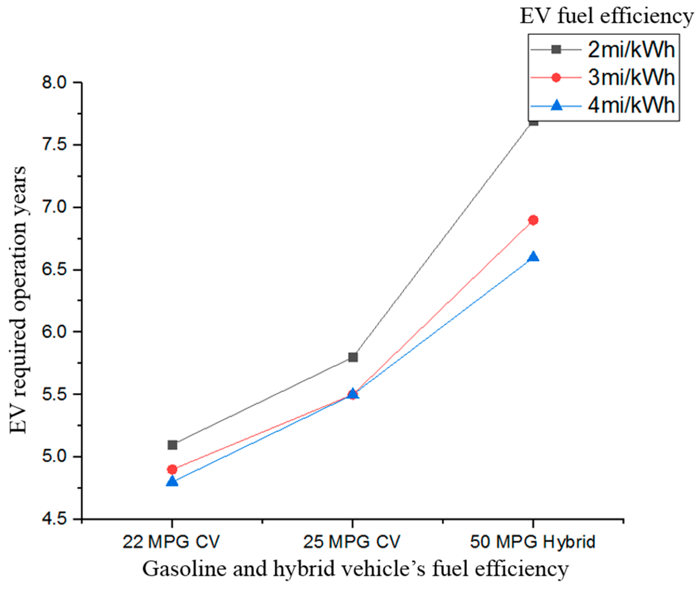
We use three different fuel efficiencies for each vehicle type to investigate how model sensitivities are affected by fuel efficiency. CVs require 22 miles per gallon (mpg), 25 mpg, and 50 mpg, the highest fuel efficiency for the Toyota Prius, a hybrid vehicle. EVs have a higher purchase price and efficiency ranges (mile per kWh) are 2 mi/kWh, 3 mi/kWh, and 4 mi/kWh. As shown in Figure 6, the EV requirement years to minimize total costs increase as CV mpg improves. That is, EVs become less competitive with the adoption of improved fuel efficiency CVs like traditional hybrids. CV required operating duration remains three years. Due to increased maintenance costs and decreased depreciation cost, the fleet would improve by selling old vehicles and buy new ones to minimize total fleet costs. The EV fuel efficiency scenarios do not differ much because of low fuel cost for EVs.
Figure 8 illustrates vehicle costs per year according to each scenario. Across all the scenarios, EVs’ total costs are less than those of gasoline vehicles. In addition, even though the mile per kWh improved, the total costs for EVs do not decrease significantly because maintenance and repair costs exceed electricity costs. In contrast, CVs show a different pattern. The improved fuel economy decreases total costs. CVs are sensitive to gasoline price or fuel economy while EVs’ mean total costs are not much affected by electricity price or mi/kWh. Unlike comparison with CVs, the total costs for EVs increased when the mile energy efficiency improved compared to hybrid vehicles. This reflects the longer duration of time EVs are kept in the fleet and a hybrid vehicle’s lower depreciation rate (when compared to CVs).
7. Conclusions
There have been no studies about the UT motor pool fleet since 1980; this study analyzes recent data and then compares the old and new fleets. The UT motor pool fleet size has increased since 1980 and the appropriate fleet size needed to be re-estimated. The trip duration pattern remains five days or less for 85% of all trips [41,42]. Additionally, a strong linear relationship between total trip mileage (mile) and duration (day or hour) also remains.
The purpose of this study has been to determine the optimized fleet size and composition through queuing and optimization modeling. While, in recent years, many research projects have developed fleet size and composition optimization models, none of these studies consider EV adoption with its unique constraints [1,2,4,46]. This study builds a queuing model to estimate the appropriate fleet size to satisfy demands, which means making the probability an arriving customer has to wait near zero. This model can estimate optimized fleet composition for a wide range of vehicle types with varying characteristic including purchase price, maintenance costs, fuel costs, travel distance, and refueling time. That information can help guide fleets as they adopt the EV or other alternative vehicles.
Results suggest that the UT motor pool may be inefficiently allocating resources. It currently operates with 95 sedans and this research shows that 51 vehicles can satisfy all demands while keeping the probability that an arriving customer has to wait at near zero. Indeed, 30 vehicles could meet 96% of trips in the dataset. The fleet can save on the total annual cost of ownership and generate revenue from sold surplus vehicles. From the analysis, the highest ownership cost occurs during the first year because of sales tax and vehicle registration. The costs gradually increase after the second year as vehicles require more maintenance and repairs, gas prices increase, and fuel efficiency decreases. When the fleet has the appropriate number of vehicles (meaning 44 fewer than it currently maintains), total annual ownership costs can be saved while maintenance is reduced and depreciation costs are minimized.
This study explores annual breakdown cost components based on different EV and CV costs. This includes different depreciation rates from real market data. Even though an EV’s depreciation rate is better than that of a CV, depreciation accounts for the largest part of EV costs. For CVs, fuel costs, along with depreciation costs, account for the largest part of CV costs.
Future research could take this model and introduce more variables, like service and waiting costs, and emission reduction benefits. This study assumes that fleet size should satisfy demands and it would be interesting to examine each demand satisfaction rate. EVs, CVs, and hybrid vehicles’ specifications and characteristics are changing and the research based on the considerations of those changes can be a good future research topic. Finally, allowing outsourced rentals (e.g., commercial rental cars) could be an area of further cost saving during peak demand times.
Although there has been a great deal of research examining fleet optimization, there is little research investigating how fleets can adopt EVs efficiently. The fleet size and composition optimization model is very flexible. It can be used for a wide variety of fleet optimization problems including fleet size and EV adoption as it was used here. It can help vehicle fleets’ demands within cost constraints and EVs’ limited travel distances.
Author Contributions
Taekwan Yoon and Christopher R. Cherry developed the optimization model and analyzed the data, and wrote the paper.
Conflicts of Interest
The authors declare no conflict of interest.
References
- Etezadi, T.; Beasley, J.E. Vehicle Fleet Composition. J. Oper. Res. Soc. 1983, 34, 87–91. [Google Scholar] [CrossRef]
- Gould, J. The Size and Composition of a Road Transport Fleet. J. Gould 1969, 20, 81–92. [Google Scholar]
- Loxton, R.; Lin, Q.; Teo, K.L. A stochastic fleet composition problem. Comput. Oper. Res. 2012, 39, 3177–3184. [Google Scholar] [CrossRef]
- Fu, L.; Ishkhanov, G. Fleet Size and Mix Optimization for Paratransit Services. Transp. Res. Rec. 2004, 1884, 39–46. [Google Scholar] [CrossRef]
- Simms, B.W.; Lamarre, B.G.; Jardine, A.K.S.; Boudreau, A. Optimal buy, operate and sell policies for fleets of vehicles. Eur. J. Oper. Res. 1984, 15, 183–195. [Google Scholar] [CrossRef]
- Funk, K.; Rabl, A. Electric versus conventional vehicles: Social costs and benefits in France. Transp. Res. Part D Transp. Environ. 1999, 4, 397–411. [Google Scholar] [CrossRef]
- Samaras, C.; Meisterling, K. Life Cycle Assessment of Greenhouse Gas Emissions from Plug-in Hybrid Vehicles: Implications for Policy. Environ. Sci. Technol. 2008, 42, 3170–3176. [Google Scholar] [CrossRef] [PubMed]
- Wirasingha, S.G.; Schofield, N.; Emadi, A. Plug-in hybrid electric vehicle developments in the US: Trends, barriers, and economic feasibility. In Proceedings of the 2008 IEEE Vehicle Power and Propulsion Conference (VPPC), Harbin, Hei Longjiang, China, 3–5 September 2008. [Google Scholar]
- Lester, L.B.; Hendrickson, C.T.; McMichael, F.C. Environmental implications of electric cars. Science 1995, 268, 993–995. [Google Scholar]
- Situ, L. Electric Vehicle development: The past, present & future. In Proceedings of the Power Electronics Systems and Applications, PESA 2009, Hong Kong, China, 20–22 May 2009. [Google Scholar]
- Shiau, C.-S.N.; Kaushal, N.; Hendrickson, C.T.; Peterson, S.B.; Whitacre, J.F.; Michalek, J.J. Optimal Plug-In Hybrid Electric Vehicle Design and Allocation for Minimum Life Cycle Cost, Petroleum Consumption, and Greenhouse Gas Emissions. J. Mech. Des. 2010, 132, 91013. [Google Scholar] [CrossRef]
- Taylor, J.; Maitra, A.; Alexander, M.; Brooks, D.; Duvall, M. Evaluation of the impact of plug-in electric vehicle loading on distribution system operations. In Proceedings of the Power & Energy Society General Meeting 2009, PES ’09, Calgary, AB, Canada, 26–30 July 2009. [Google Scholar]
- Mozafar, M.R.; Amini, M.H.; Moradi, M.H. Innovative appraisement of smart grid operation considering large-scale integration of electric vehicles enabling V2G and G2V systems. Electr. Power Syst. Res. 2018, 154, 245–256. [Google Scholar] [CrossRef]
- Yoon, T.; Cherry, C.R.; Jones, L.R. One-way and round-trip carsharing: A stated preference experiment in Beijing. Transp. Res. Part D Transp. Environ. 2017, 53, 102–114. [Google Scholar] [CrossRef]
- Nissan USA. Available online: http://www.nissanusa.com/ (accessed on 14 March 2014).
- Amini, M.H.; Islam, A. Allocation of electric vehicles’ parking lots in distribution network. In Proceedings of the 2014 IEEE PES Innovative Smart Grid Technologies Conference (ISGT), Washington, DC, USA, 19–22 February 2014. [Google Scholar]
- Delucchi, M.A. Environmental Externalities of Motor-Vehicle Use in the US. J. Transp. Econ. Policy 2000, 34, 135–168. [Google Scholar]
- Parrish, D.D. Critical evaluation of US on-road vehicle emission inventories. Atmos. Environ. 2006, 40, 2288–2300. [Google Scholar] [CrossRef]
- Rexeis, M.; Hausberger, S. Trend of vehicle emission levels until 2020—Prognosis based on current vehicle measurements and future emission legislation. Atmos. Environ. 2009, 43, 4689–4698. [Google Scholar] [CrossRef]
- Dill, J. Estimating emissions reductions from accelerated vehicle retirement programs. Transp. Res. Part D Transp. Environ. 2004, 9, 87–106. [Google Scholar] [CrossRef]
- Kim, H.C.; Keoleian, G.A.; Grande, D.E.; Bean, J.C. Life Cycle Optimization of Automobile Replacement: Model and Application. Environ. Sci. Technol. 2003, 37, 5407–5413. [Google Scholar] [CrossRef] [PubMed]
- Hadley, W.S.; Tsvetkova, A.A. Potential Impacts of Plug-in Hybrid Electric Vehicles on Regional Power Generation. Electr. J. 2009, 22, 56–68. [Google Scholar] [CrossRef]
- Sims, R.E.H.; Rogner, H.-H.; Gregory, K. Carbon emission and mitigation cost comparisons between fossil fuel, nuclear and renewable energy resources for electricity generation. Energy Policy 2003, 31, 1315–1326. [Google Scholar] [CrossRef]
- Crevier, B.; Cordeau, J.-F.; Laporte, G. The multi-depot vehicle routing problem with inter-depot routes. Eur. J. Oper. Res. 2007, 176, 756–773. [Google Scholar] [CrossRef]
- Baldacci, R.; Toth, P.; Vigo, D. Recent advances in vehicle routing exact algorithms. Q. J. Oper. Res. 2007, 5, 269–298. [Google Scholar] [CrossRef]
- Gendreau, M.; Iori, M.; Laporte, G.; Martello, S. A Tabu search heuristic for the vehicle routing problem with two-dimensional loading constraints. Networks 2008, 51, 4–18. [Google Scholar] [CrossRef] [Green Version]
- Eksioglu, B.; Vural, A.V.; Reisman, A. The vehicle routing problem: A taxonomic review. Comput. Ind. Eng. 2009, 57, 1472–1483. [Google Scholar] [CrossRef]
- Côté, J.-F.; Potvin, J.-Y. A tabu search heuristic for the vehicle routing problem with private fleet and common carrier. Eur. J. Oper. Res. 2009, 198, 464–469. [Google Scholar] [CrossRef]
- Laporte, G. Fifty Years of Vehicle Routing. Transport. Sci. 2009, 43, 408–416. [Google Scholar] [CrossRef]
- Golden, B.L. Route planning for coast guard ships. Manage. Sci. Syst. 1988, 16, 439–444. [Google Scholar]
- Toth, P.; Vigo, D. The Vehicle Routing Problem; Society for Industrial and Applied Mathematics: Philadelphia, PA, USA, 2001. [Google Scholar]
- Golden, B.L.; Raghavan, S.; Wasil, E.A. The Vehicle Routing Problem: Latest Advances and New Challenges; Springer: Berlin, Germany, 2008; Volume 43. [Google Scholar]
- Vidal, T.; Crainic, T.G.; Gendreau, M.; Prins, C. Heuristics for Multi-Attribute Vehicle Routing Problems: A Survey and Synthesis. Eur. J. Oper. Res. 2012, 231, 1–21. [Google Scholar] [CrossRef]
- Golden, B.L.; Wong, R.T. Capacitated arc routing problems. Networks 1981, 11, 305–315. [Google Scholar] [CrossRef]
- Baldacci, R.; Battarra, M.; Vigo, D. Routing a heterogeneous fleet of vehicles. In The Vehicle Routing Problem: Latest Advances and New Challenges; Springer: Berlin, Germany, 2008; Volume 43, pp. 3–27. [Google Scholar]
- Baldacci, R.; Mingozzi, A. A unified exact method for solving different classes of vehicle routing problems. Math. Program. 2009, 120, 347–380. [Google Scholar] [CrossRef]
- Choi, E.; Tcha, D.-W. A column generation approach to the heterogeneous fleet vehicle routing problem. Comput. Oper. Res. 2007, 34, 2080–2095. [Google Scholar] [CrossRef]
- Brandão, J. A tabu search algorithm for the heterogeneous fixed fleet vehicle routing problem. Comput. Oper. Res. 2011, 38, 140–151. [Google Scholar] [CrossRef]
- Prins, C. A GRASP× evolutionary local search hybrid for the vehicle routing problem. In Bio-Inspired Algorithms for the Vehicle Routing Problem; Part of the Studies in Computational Intelligence Book Series; Springer: Berlin, Germany, 2009; Volume 161, pp. 35–53. [Google Scholar]
- Penna, P.H.V.; Subramanian, A.; Ochi, L.S. An iterated local search heuristic for the heterogeneous fleet vehicle routing problem. J. Heuristics 2013, 19, 201–232. [Google Scholar] [CrossRef]
- Williams, W.; Fowler, O. Minimum Cost Fleet Sizing for a University Motor Pool. Interfaces 1980, 10, 21–29. [Google Scholar] [CrossRef]
- Williams, W.W.; Fowler, O.S. Model formulation for fleet size analysis of a university motor pool. Decis. Sci. 1979, 10, 434–450. [Google Scholar] [CrossRef]
- US Department of Energy. Available online: http://www.energy.gov/ (accessed on 14 March 2013).
- KBB.com Web. Used Car Resale Value. 2018. Available online: kbb.com (accessed on 9 January 2018).
- Stevenson, W.J.; Hojati, M. Operations Management; McGraw-Hill/Irwin Boston: Boston, MA, USA, 2007; Volume 8. [Google Scholar]
- Golden, B.; Golden, B.; Assad, A.; Levy, L.; Gheysens, F. The fleet size and mix vehicle routing problem. Comput. Oper. Res. 1984, 11, 49–66. [Google Scholar] [CrossRef]
Figure 1.
Schematic overview.

Figure 2.
The frequency of the number of vehicles checked out simultaneously.

Figure 3.
Depreciation rates by vehicle age and model (data source: Kelly Blue Book).

Figure 4.
Break-even point (example).

Figure 5.
Simulation flow.
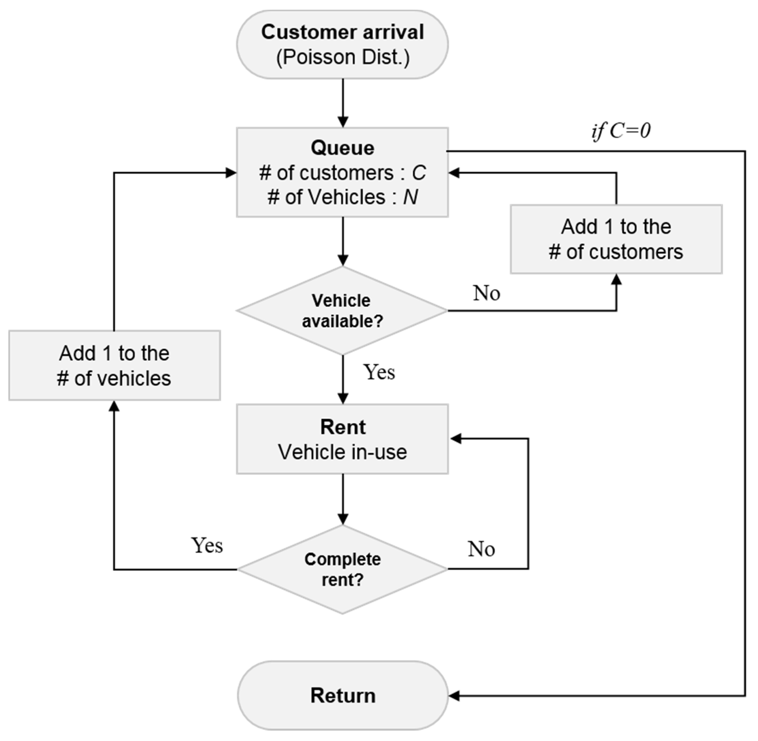
Figure 6.
Probability an arriving customer has to wait in queuing theory.
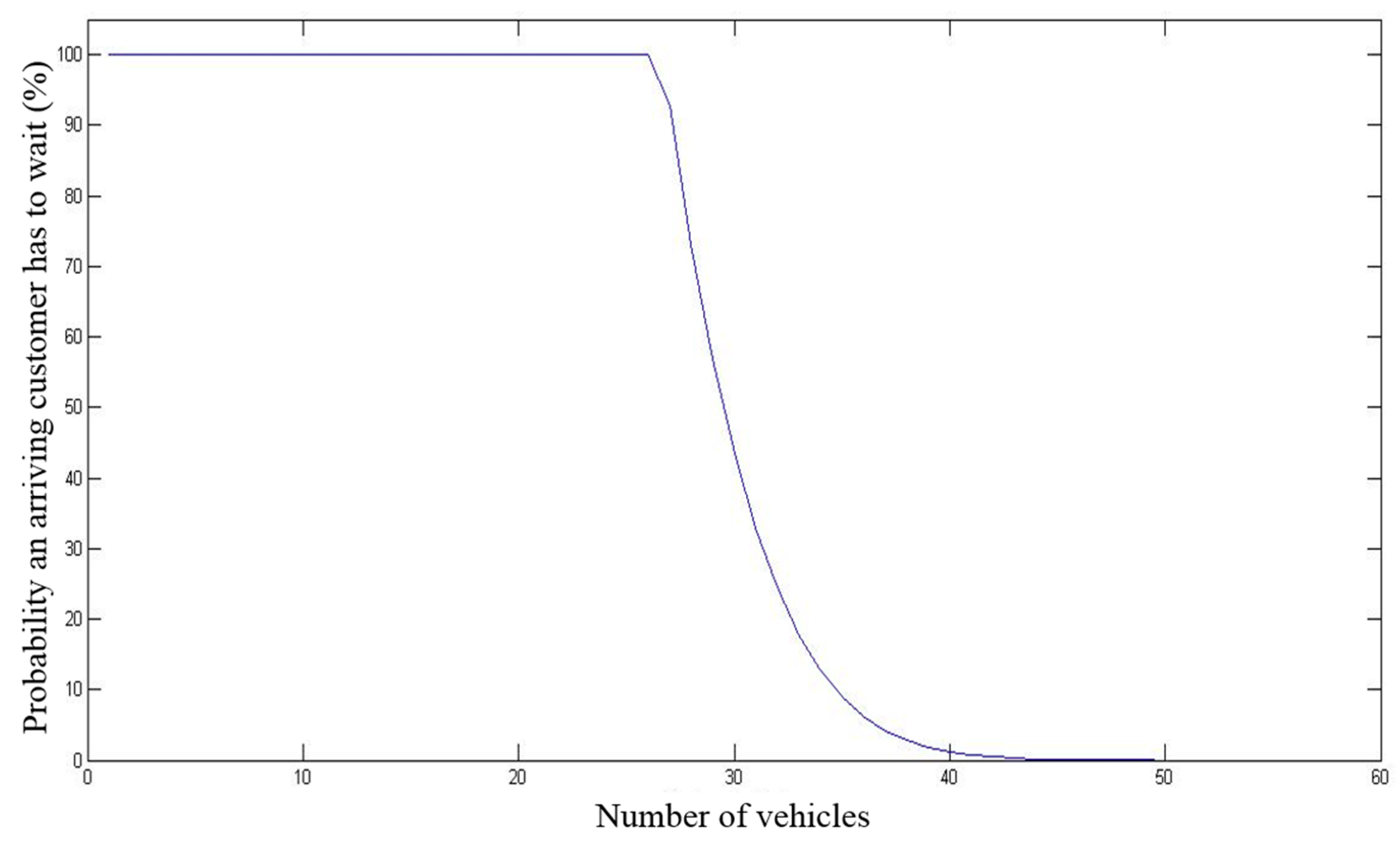
Figure 7.
Detailed break-down cost elements of (a) CV (conventional vehicle) and (b) EV (electric vehicle) per year.
Figure 7.
Detailed break-down cost elements of (a) CV (conventional vehicle) and (b) EV (electric vehicle) per year.

Figure 8.
EV required operating years against mi/kWh and mpg to break even with CV.

Table 1.
Break-even point.
| Assumptions | 20,000 miles Per Year, Gasoline Price: $3.25/gal, Electricity Price: $0.10/kWh (10 Years, 5% Discount Rate) | |||
|---|---|---|---|---|
| EV (Chevrolet Volt) | CV (Dodge Avenger) | |||
| No Subsidy | Subsidy (TN) | Subsidy | - | |
| MSRP ($) | 34,095 | 19,900 | ||
| Subsidy ($) | 0 | 2500 | 7500 | 0 |
| Tax and registration (7%) ($) | 2387 | 2212 | 1862 | 2464 |
| Total purchase price ($) | 36,482 | 33,807 | 28,457 | 21,293 |
| Fuel cost/year ($) | 666.67 | 2600.00 | ||
| Maintenance costs ($) | 200 ($0.01/mile) | 1600 ($0.08/mile) | ||
| Depreciations | Data from Kelly Blue Book | |||
| BEP (years) | 4.56 | 3.75 | 2.15 | - |
Table 2.
Optimization results.
| Number of Vehicles | Travel Mileage Per Year | Years Need to be Operated | Total Costs/Vehicle/Year (Resale Value Included) | |
|---|---|---|---|---|
| EVs | 7 | 10,218 miles | 4.5 | $6062 |
| Gasoline Vehicles | 44 | 20,193 miles | 3 | $10,116 |
© 2018 by the authors. Licensee MDPI, Basel, Switzerland. This article is an open access article distributed under the terms and conditions of the Creative Commons Attribution (CC BY) license (http://creativecommons.org/licenses/by/4.0/).
Share and Cite
MDPI and ACS Style
Yoon, T.; Cherry, C.R. Migrating towards Using Electric Vehicles in Campus-Proposed Methods for Fleet Optimization. Sustainability 2018, 10, 285. https://doi.org/10.3390/su10020285
AMA Style
Yoon T, Cherry CR. Migrating towards Using Electric Vehicles in Campus-Proposed Methods for Fleet Optimization. Sustainability. 2018; 10(2):285. https://doi.org/10.3390/su10020285
Chicago/Turabian StyleYoon, Taekwan, and Christopher R. Cherry. 2018. "Migrating towards Using Electric Vehicles in Campus-Proposed Methods for Fleet Optimization" Sustainability 10, no. 2: 285. https://doi.org/10.3390/su10020285
Note that from the first issue of 2016, this journal uses article numbers instead of page numbers. See further details here.