Recurrence Interval Analysis on Electricity Consumption of an Office Building in China


1
School of Electrical Engineering, Southeast University, Nanjing 210096, Jiangsu, China
2
School of Management and Economics, Southeast University, Nanjing 210096, Jiangsu, China
*
Author to whom correspondence should be addressed.
Sustainability 2018, 10(2), 306; https://doi.org/10.3390/su10020306
Submission received: 30 November 2017
/
Revised: 11 January 2018
/
Accepted: 12 January 2018
/
Published: 24 January 2018
(This article belongs to the Special Issue Sustainable Electric Power Systems Research)
Abstract
:The energy management of office buildings has been a rising concern for owners, researchers, and energy suppliers. The volatility of power load in office buildings threatens energy consumption and risks device security. This paper investigates the load fluctuation patterns in an office building based on user data, using recurrence interval analysis for different thresholds. The recurrence intervals of volatility are fitted by stretched exponential distribution, from which the probability density function is derived. Then, the short-term and long-term memory effect on the fluctuations are learned by conditional probability density function and multifractal detrended fluctuation analysis, respectively. A hazard function is further established to analyze the risk estimation of load volatility and derive the value at risk (VaR). Thus, a functional relationship has been established between average recurrence interval and threshold. The methodology and analysis results addressed in this paper help to understand load fluctuation patterns and aid in the design of energy consumption strategies in office buildings. According to the results of our research, conclusions and management suggestions are provided at the end of this paper.
1. Introduction
The excessive energy consumption of office buildings is becoming a critical and urgent problem in urban development. According to the ministry of construction and other related research departments, China has experienced a rapid development in the scale of construction which has resulted in poor heat preservation performance in new buildings. Hence, the energy consumption of high-rise buildings in the heating-cooling process is much higher than the global average, which makes it urgent to strengthen energy management for office buildings and promote the rational and efficient utilization of energy [1,2].
At present, one-third of total societal energy consumption goes to buildings in the developed world. Though the amount is less than in these developed countries, the proportion of energy consumption in Chinese buildings has increased in recent years due to the rapid development of the construction market. It is forecasted that the number of large public buildings in China (e.g., offices, apartments, restaurants, convention centers, and others) will rise dramatically in the next few years, and China will add an area of about 1 billion square meters of large public buildings by 2020. It is estimated that more than 90% of the large public buildings in China are large energy (electricity) consumers [3]. Thus, in confronting the increasing energy demand, it is unavoidable that we must realize building energy management by various means so as to reduce the energy dissipation of the buildings, including lighting, air conditioning, power, special equipment, and other energy consumption, which has become the most concerning problem for building owners.
In recent years, China’s national economy has developed rapidly, with a high daily electricity consumption whose peak appears during the daytime, especially in summer. Large companies, shopping malls, office buildings, and other buildings need air-conditioning systems to adjust the temperature. Hence, daytime electricity demands and prices are both much higher than those at night. With the advancement of science and technology, the ice thermal storage system has been used at night to avoid electricity reaching its peak during the day. This helps to reduce electricity consumption during peak hours and increases power off-peak consumption, which is called peak load shifting. This saves money for businesses and promotes local economic development [4].
Energy management reflects the quantified data of energy conservation and plays an important role in emission reduction. Meanwhile, it contributes to applying the energy data as a management tool and means for accurate diagnosis and analysis and promotes the utilization of construction energy, resulting in energy savings in office buildings.
As one of the indispensable developments in social energy, electricity is considered of great significance to the economy. At present, China has an urgent demand to save resources as the world’s second-largest power consumer. Therefore, the forecast on power load has become an important research focus and has been investigated continuously in recent years, from which power suppliers and consumers can benefit to develop better energy management. The forecasting period ranges from minutes to years due to the various demands for power load forecasting [5,6,7]. Many models have been developed to address this problem, and most of them can be classified into three categories: regression models, time series analysis, and artificial neural networks (ANNs).
Regression models make use of linear functions to construct relationships between the dependent variables and numerous independent variables, including weather [8], income [9], GDP (Gross Domestic Product), and seasonal variables [10]. The validity and correctness of regression models have been confirmed by some empirical studies [11,12]. This modeling method and its extended versions are widespread among researchers since they can accurately quantify the effect caused by various factors. Today, abstract characteristics such as human behavior can also be physically described thanks to technological development, although the model accuracy is sensitive to the volume of data.
Unlike the regression model, time series analysis considers future power load as a function of previous load [13]. Typical time series analysis models consist of a multiplicative autoregressive model, an autoregressive integrated moving average, and an autoregressive moving average with exogenous input model [14]. Though the model is effective in short-time load prediction, its requirement for the accuracy of historical data is extremely high, and the algorithm may be complex and unstable in some nonlinear or non-stationary cases. Further, when involving meteorological factors, time series analyses are unable to deal with the inaccuracy problems.
Compared to time series analysis, ANNs require further investigations [15]. An ANN does not presume functional relations between past and future electrical loads, and performs better in dealing with nonlinear and non-stationary relationships [16]. Benefiting from its great extensibility, ANNs can integrate various other tools, including genetic algorithms [17], fuzzy logic [18], wavelet analysis [19], and grey systems [20]. The effectiveness of ANNs has been confirmed in several case studies [21,22]. Currently, ANNs are widely applied in various fields consisting of electrical loads forecasting, although ANNs are associated with the problems of slow convergence speed and the danger of easily falling into local minima.
In this paper, recurrence interval analysis (RIA) [23]—which belongs to the category of time series analysis—is introduced to investigate the fluctuation patterns of energy consumption in office buildings. RIA focuses on the time interval of volatility instead of the power load. Therefore, RIA enables us to analyze the profile of volatility in different magnitudes, and it does not have to make the presumption that the load between past and future should follow specific functional relationships [23]. Owing to its wide application, RIA is now used in diverse fields, including the study of climate [24], earthquake activities [25], heartbeat monitoring [26], and financial volatility [27].
Electricity generation requires the development of annual, monthly, daily, and even hourly power system generation planning. Generation ability satisfies most needs for power in cities, but managers are more concerned with fluctuations. Since traditional turbo generators cannot be regulated instantly, surging and collective loads will disrupt the supply balance of power systems and lead to electricity supply halts.
In the grid, it is important to design the power capacity of transmission lines and devices, and load fluctuation makes capacity design more complex and equipment more expensive with “redundant” performance, while the rate of return on investment is less. In addition, when out of normal range, fluctuations can result in bus voltage out-of-limits and vulnerable power quality and interrupt the normal work of some sensitive instruments.
In the power market, the load of a single building may have little effect on the power grid, but considering the process of Chinese urbanization and its countless buildings in cities, multiple load fluctuations at the same time will threaten the security of the energy supply. With regard to electricity market reform in China, both the amount and the volatility of the power load are essential and of great value to formulate a suitable energy supply strategy and reduce the running cost of buildings.
It is therefore reasonable to find that the system is threatened by risks of violent fluctuations. The rest of this paper is arranged as follows. In Section 2, the analysis method is proposed and the basic statistics of the dataset are presented. Then, an empirical study, including distribution function, scaling properties, memory effect, and risk estimation, is demonstrated in Section 3, while the conclusions of this paper are delivered in Section 4.
2. Method
“Recurrence interval” refers to the time interval between two sequential events beyond (below) a positive (negative) threshold, and is usually utilized to investigate the extreme events among the fluctuations. As is well known, extreme events feature a huge magnitude with a lower occurrence probability, in accordance with the reality in the field of power research. Different from the financial market, where investors mostly pay attention to price decline, electricity suppliers/consumers care more about power load volatility.
A typical office building possesses heating, ventilation, and air conditioning systems that consume a large portion of electricity [28]. RIA on extreme events with regard to electricity load fluctuation helps to better forecast the future energy load, which can be applied to formulate a power supply/consumption strategy.
2.1. Research Object Information
Today, commerce buildings are common in urban areas due to the development of China’s reform and opening up, as well as improvements to the standard of living in China. The office building selected as the research object is located in Xuanwu District, Nanjing, Jiangsu, China. The construction area of the building is about 133 thousand square meters, which meets the multiple demands of international enterprises. The building has a total height of 58 floors, of which floors 1–5 are a shopping/leisure plaza, floor 6 includes large restaurants, floors 7–8 are hotel auxiliary facilities (including a swimming pool, gymnasium, Western restaurant, and conference center), floors 9–26 are hotel suites, and floors above 26 contain office space—all of which are rentals and are not for sale.
The power load data collected in this paper come from the meters in the office building area, and were telemetry-recorded at a 15-min frequency by the State Grid Nanjing Electric Power Company. The sample period covers from 1 January 2016 through 31 December 2016, and the data collected are comprised of 35,111 electricity load observations.
2.2. Fluctuation of Power Load
The return of time series is calculated by taking the logarithmic difference of the load, as follows:
In Equation (1), is the electricity load (unit: kW) of th time, and because of the data sampling frequency. The logarithmic return reduces the absolute value of the data and makes the calculation convenient, which allows the multiplication to be transformed into an addition calculation. It does not change the nature and correlation of the data, and helps to weaken the collinearity and heteroscedasticity of the model, making further statistical analysis possible.
To apply the recurrence interval analysis, time series is normalized by dividing its standard deviation as follows:
where E denotes the mathematical expectation of the variables and is the standard deviation of . For each threshold , a group data of recurrence interval can be obtained, with which the probability density function of is confirmed. Therefore, the mathematical expression of the recurrence interval could be derived as follows:
2.3. Probability Density Function
Considering as the recurrence interval when the threshold is , the overwhelming consensus [27,29,30] is that the recurrence intervals of volatility can be fitted by a stretched exponential distribution, which is given by
Equation (4) means that, given a threshold , the distribution of recurrence interval is , where is the mean recurrence interval depending on , and , , and are the function parameters.
2.4. Memory Effect
2.4.1. Short-Term Memory
To investigate short-term correlations among the recurrence intervals, , the conditional probability density functions are first calculated and compared. is the probability of finding a recurrence interval immediately following the recurrence interval . The criterion is that if there are no short-term correlations, will be found independent from . However, in order to obtain more data, values of for in a certain interval will be calculated instead of a single value of [31].
For a given threshold q, the set of all the recurrence intervals is partitioned into four non-overlapping subsets, meeting where . All of the recurrence intervals in are sorted with an increasing order in the partitioning procedure, and then T is turned into subsets with the same size. Hence, the quarter smallest recurrence intervals are selected to the first subset , while contains the largest quarter of T. Under the estimation that the conditional probability density functions are derived as , and if there are no short-term correlations, it can be found that .
2.4.2. Long-Term Memory
The multifractal detrended fluctuation analysis (MF-DFA) method [32,33] is adopted to determine the long-term memory in electricity consumption for Building A.
The conventional DFA method—invented by Peng to investigate the long-range dependence in DNA nucleotide sequences [34]—is adopted in this paper to investigate the statistical self-affinity in time series analysis. The properties of DFA have been extensively studied, and have been authenticated to be capable of characterizing the long-term correlations in a time series [35,36,37]. Kantelhardt [32] combined multifractal with DFA and proposed MF-DFA, which allows us to describe the multifractal characteristics of time sequence and compute the Hurst exponent H(p) for all p-order statistical moments. When p = 2, the MF-DFA degrades into conventional DFA.
For a non-stationary time series, only when 0.5 < H(p) < 1 will the series have a long-term correlation, indicating that the system has a fluctuation pattern in long-term evolution. When H(p) is the function of p, the time series has multiple fractal characteristics.
2.5. Risk Estimation
The hazard probability function is one important method to estimate risk in recurrence interval analysis. Considering the fact that t units of time have passed since the last large volatility greater than , it is probable that the next large volatility greater than will occur within units of time. Mathematically, the hazard probability function can be expressed as
Since each distribution has been matched to a stretched exponential, the theoretical value of can be calculated with the parameters , as shown in Equation (4). Besides, in order to determine the empirically, is further derived as
where “” denotes the number of recurrence intervals greater than units of time and “” is the number of recurrence intervals greater than and not greater than for a given .
Value at risk (VaR) is widely applied for risk estimation. In this paper, the loss probability density function in RIA is introduced to estimate the VaR, which defines the risk at loss as follows:
where is probability density function of the normalized series and is the loss probability. Then, the mean recurrence interval can be derived as
where denotes the number of intervals that fall below the threshold , so is approximately equal to the total number of returns, and is the number of returns below threshold . Thus, the mean recurrence interval can satisfy VaR as
3. Results
The fluctuations of logarithmic returns of power load in the office building are presented in Figure 1, and the statistics are calculated as shown in Table 1.
From Figure 1, it is found that the returns are not normally distributed and sharp peaks arise. In Table 1, the volatility is not symmetric, and the magnitude of negative values are higher than that of positive values. It is also observed that volatile time periods when large volatilities cluster are accompanied by short and dense recurrence intervals. In contrast, the recurrence during calm periods with small volatility intervals are large and sparse. In the meantime, the volatility clusters (i.e., large fluctuations) tend to follow a large fluctuation, while the small ones tend to follow small ones, which helps to demonstrate the existence of long-term memory. Moreover, we go further to wonder whether there are multi-fractal properties—namely, self-similarity—in the volatilities.
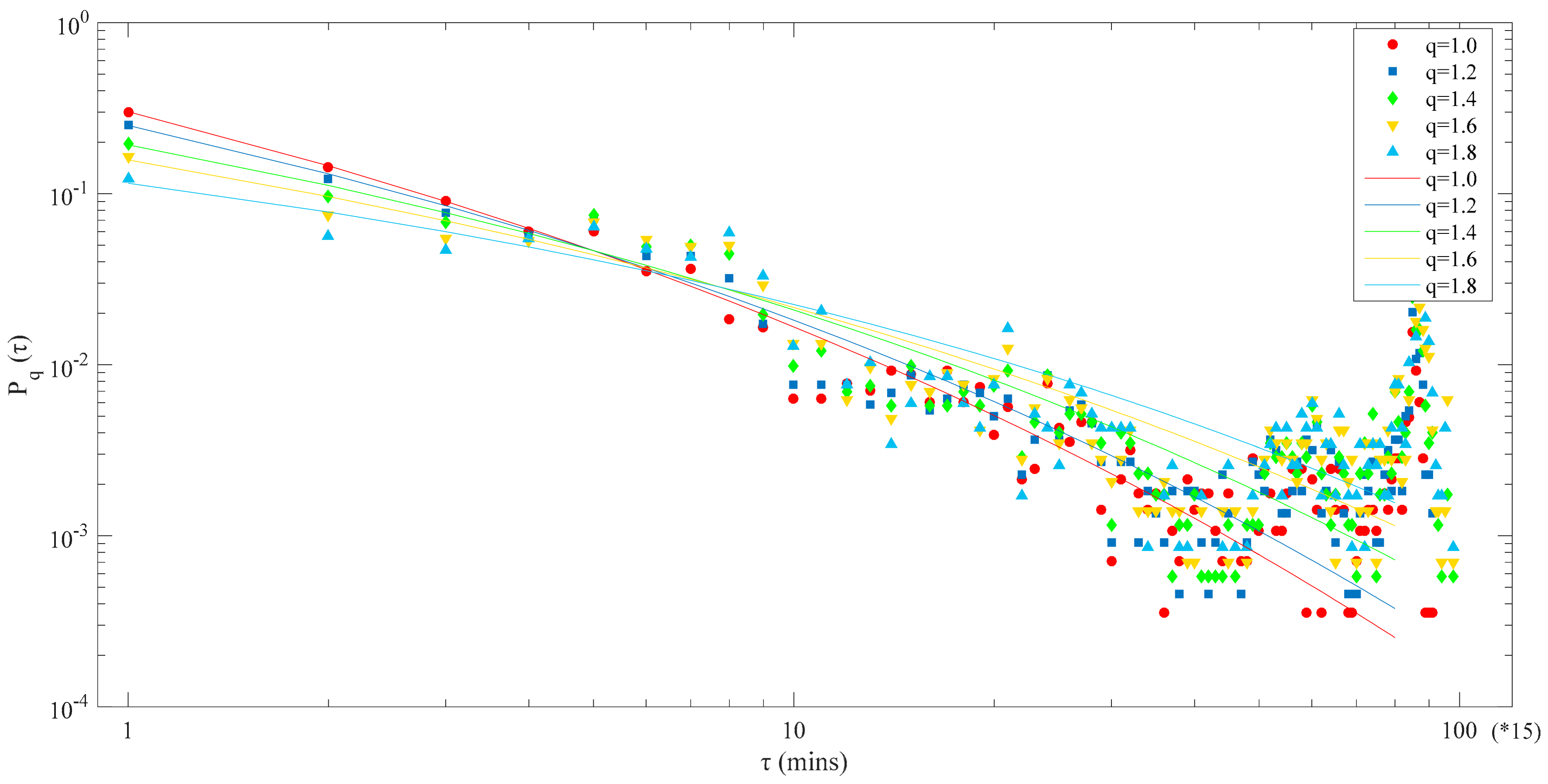
Figure 2 depicts the , the distribution of recurrence interval , between returns with different threshold , of which the parameters are also calculated by maximum likelihood estimation, as shown in Table 2.
From Figure 2, it can be seen that recurrence intervals will be longer with increasing , in agreement with the fact that large fluctuations have more long intervals and fewer short intervals than small fluctuations, which means the time interval between two consecutive events for large fluctuations has a higher probability of increasing than shrinking. It is observed in Figure 2 that the empirical distribution has a slight rise but then falls down again. This indicates that when the recurrence interval reaches a spot, the corresponding occurrence probability will have a slight and short increase. The magnitude of the rise in Figure 2 is too obvious to ignore, but please note that Figure 2 is in double logarithmic coordinates, and when we change it to regular logarithmic coordinates, it is merely a negligible error between theory and reality. Besides, through the analysis of Table 2 and Figure 2, it is found that all of the function curves have a similar shape, which makes us wonder if there are any scaling behaviors between these probability distribution functions (PDFs).
To examine that, the method used in Yamasaki et al. [38] is introduced into this paper as
where is the scaled recurrence interval and is the scaled PDFs. When threshold changes, will change, and there is , indicating that the mean time of recurrence interval increases with the volatility increase. Assuming is independent of , there will be a unique function for different threshold , which can be derived as
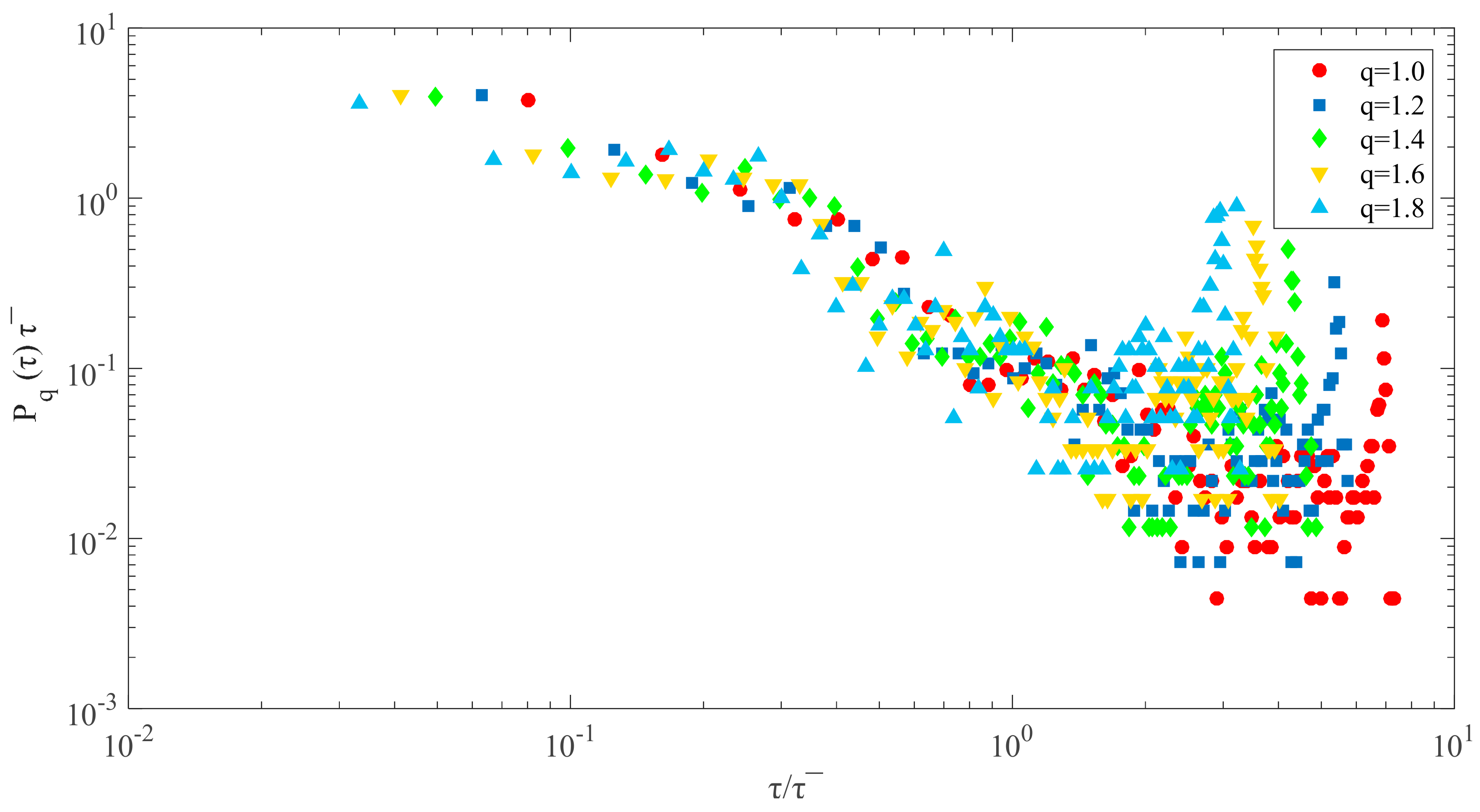
Namely, the scaled probability distribution will converge to the single curve , and recurrence intervals will show scaling behavior. To verify that, the scatter diagram of designed as the function of is shown in Figure 3.
It can be clearly seen in Figure 3 that for different thresholds , does not converge to any single curve, illustrating that there is no scaling behavior, and the behaviors of large fluctuations cannot be deduced by that of small fluctuations.
Figure 4 shows the results of as a function of for in the smallest subset (filled symbols) and the largest subset (open symbols), in which . It is also noticed that is larger than for small , while is smaller than for large . The fact that a small tends to follow a small , and a large tends to follow a large , indicates the short-term correlations in recurrence intervals.
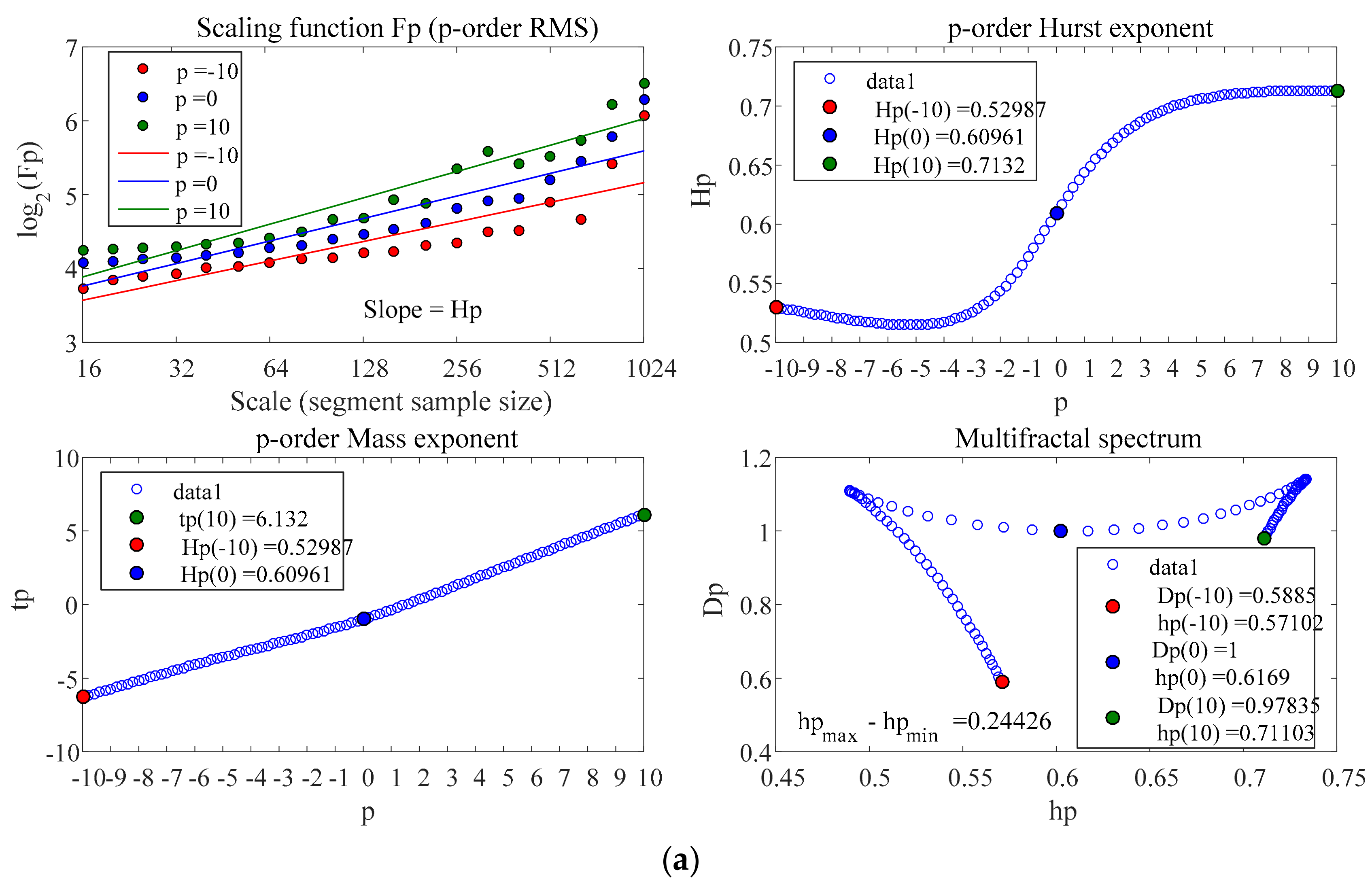
In Figure 5, there are five subfigures, and each subfigure has four sub-subfigures which show the results of MF-DFA, respectively. It can be seen that the p-order Hurst exponent of each line is greater than 0.5 in a certain area, suggesting that long-term correlations and multifractal characteristics exist in the recurrence intervals. When , it means the volatility is of anti-continuity.
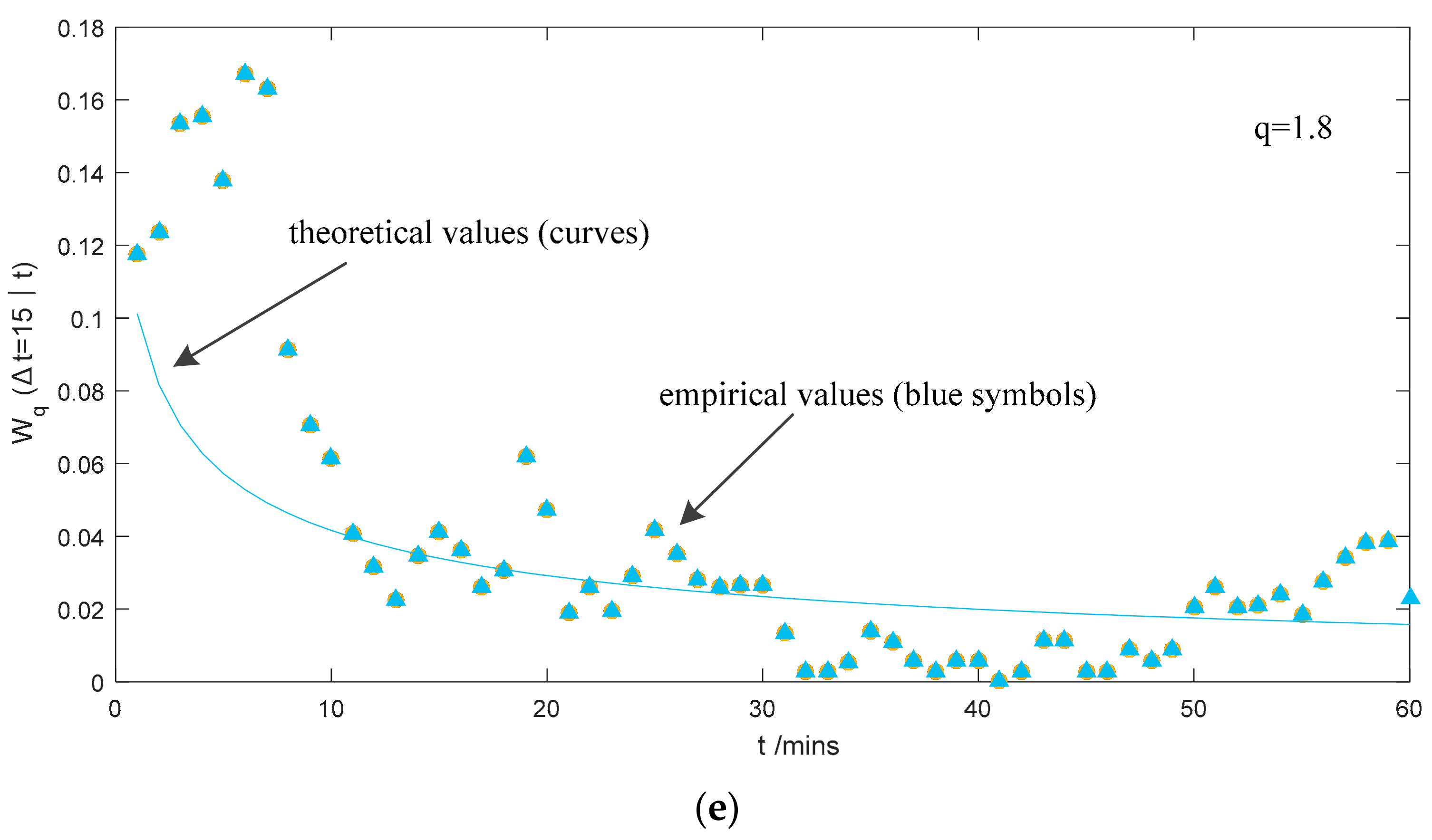
Figure 6 depicts the hazard function, in which the symbols are empirical values and the curves are the theoretical values of . It is observed that the empirical values and the curves coincide with each other very nicely, and the discrepancy between empirical and theoretical curves decreases when increases.
Furthermore, the trend that decreases with increasing suggests that recurrence intervals exhibit clustering behaviors, and long-term memory between volatilities and theoretical values will underestimate the risk in a short time period. Theoretically, the recurrence probability of extreme events can be calculated for a given threshold .
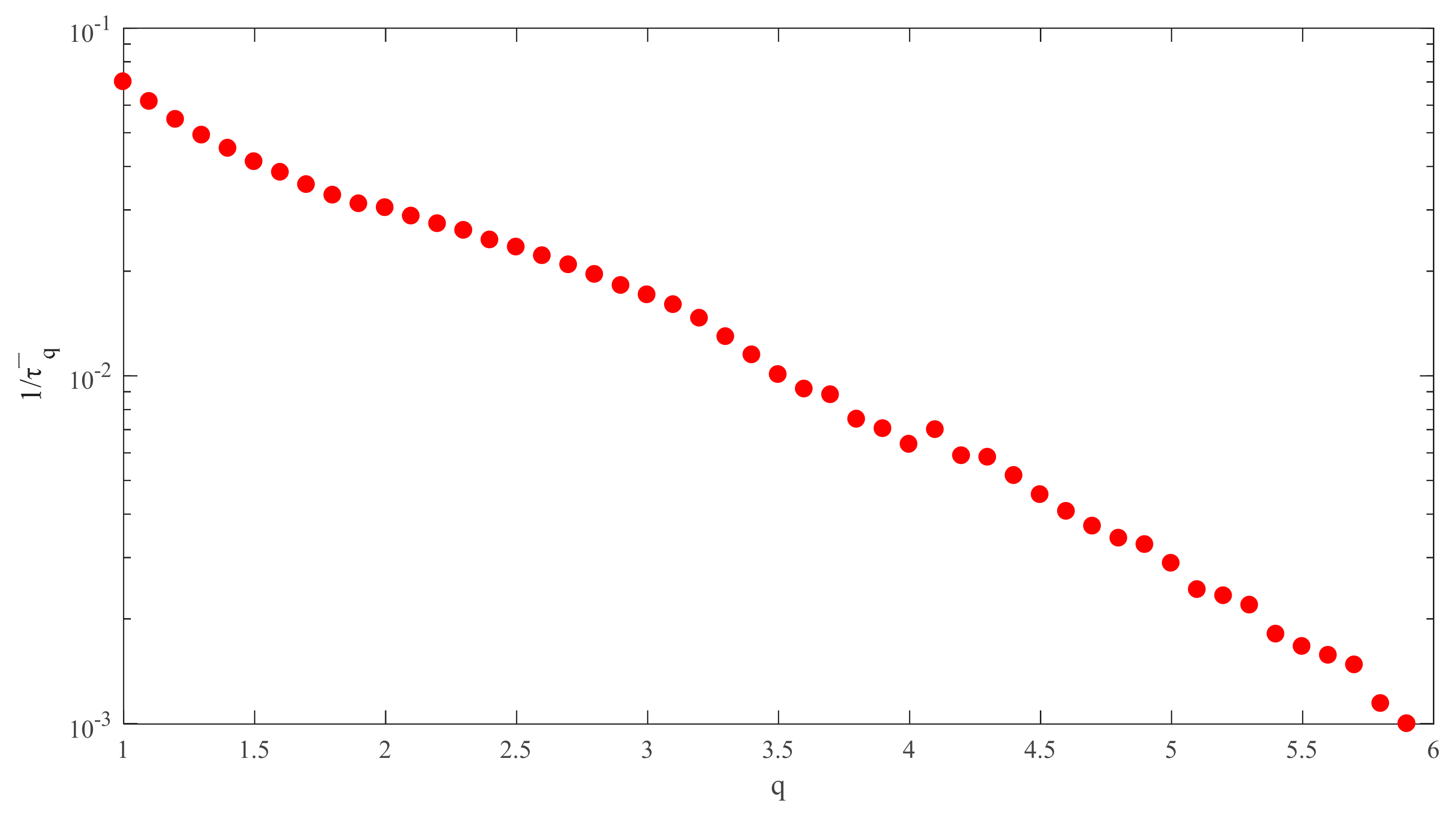
Equation (9) defines as the loss probability for a threshold , the curve of which is depicted in Figure 7. Figure 7 demonstrates the functional relationship between threshold q and the average recurrence interval.
In Figure 7, as q increases, the average recurrence interval gets larger. This illustrates that with increased volatility, the recurrence interval between load fluctuations exceeding the threshold will become larger, which is consistent with the fact that small fluctuations (with less q) are more frequent than the violent fluctuations as shown in Figure 1. Thus, energy managers can roughly estimate the risk probability of the next occurrence of different amplitude fluctuations based on (9) and Figure 7. For example, if investors want to know the probability of a risk level at 1%, they can find the q for , which represents the VaR that we are looking for.
4. Conclusions
The paper utilizes recurrence interval analysis to investigate the properties of recurrence intervals’ volatility for different thresholds and to study the power load behaviors of large volatilities in an office building from which mass data were collected at 15-min high-frequency. The RIA method was applied to analyze the characteristics of volatility in Building A and to verify the short-term and long-term memory effectiveness and estimate the VaR.
On the basis of the above empirical analyses, the following suggestions are summarized for the future improvement of China’s power supply companies and energy managers:
First, power enterprises can make full use of data to conduct load and customer management. The load of the office building fluctuates more frequently in specific periods, such as late spring and early summer and late autumn (see Figure 1), when building managers can practice seasonal differential management. More frequent and careful inspections will help to decrease the risk of serious accidents. Besides, the capacity of power devices can be optimized to save equipment costs according to the fluctuation amplitude of power loads in different areas. The details of load fluctuation and their characteristics in variable industries—including buildings—can also help to construct different energy services with industrial differences.
Second, the distribution of the probability density function is shown in Figure 2, Figure 3 and Figure 4, illustrating that the occurrence of large fluctuations can be estimated according to load fluctuation characteristics in the office building. Based on the probability density function, power enterprises can characterize the features of load fluctuations and provide it as a value-added service to large electricity consumers, which helps to reduce the operating costs. According to the estimation, power enterprises can design multiple energy storage devices or maintenance strategies for different service combinations. This will improve the efficiency of energy utilization in the region and improve the viability of the power enterprises under market-oriented reform.
Third, both short-term and long-term memory effects exist in the fluctuations in the office building, indicating that clusters of recurrence intervals of volatilities are caused by both present and long-term correlations. This helps to demonstrate that the failure of load forecasting is in some cases influenced by complicated factors.
Finally, the study of risk estimation shows that there is more short-term correlation between the recurrence intervals of power fluctuation in the office building. Therefore, when the load of the office buildings fluctuates (especially in the case of large fluctuations), energy managers need to prepare for the next similar fluctuation within a short time. Further, power supply enterprises can make corresponding preventive management strategies in order to deal with the crisis brought by sudden load fluctuations in such industries and set reasonable prices for different levels of energy usage.
This paper has some deficiencies, which can be overcome by subsequent research. Comprehensive analysis and comparison of power load fluctuations in multiple buildings can help energy suppliers and consumers realize energy management better.
Acknowledgments
This work was supported by the National Natural Science Foundation of China under Grant 51707034, and the Natural Science Foundation of Jiangsu Province under Grant BK20160679.
Author Contributions
Lucheng Hong conceived and designed the analysis method of this paper. He also conducted the critical verifications and proposed the analytical results. Wantao Shu collected the data and contributed to the words. Angela C. Chao provided instructions and valuable suggestions for this article.
Conflicts of Interest
The authors declare no conflict of interest.
References
- Bedir, M.; Kara, E.C. Behavioral patterns and profiles of electricity consumption in dutch dwellings. Energy Build. 2017, 150, 339–352. [Google Scholar] [CrossRef]
- Bedir, M.; Hasselaar, E.; Itard, L. Determinants of electricity consumption in Dutch dwellings. Energy Build. 2013, 58, 194–207. [Google Scholar]
- Guo, X.-L.; Jin, L.-Y.; Pan, J.C. Development of Workbench Interface of Power Management System Based on iFIX5.1. Value Eng. 2017, 2017, 216–219. [Google Scholar]
- Amara, F.; Agbossou, K.; Dubé, Y.; Kelouwani, S.; Cardenas, A.; Bouchard, J. Household electricity demand forecasting using adaptive conditional density estimation. Energy Build. 2017, 156, 271–280. [Google Scholar] [CrossRef]
- Cerjan, M.; Matijas, M.; Delimar, M. Dynamic Hybrid Model for Short-Term Electricity Price Forecasting. Energies 2014, 7, 3304–3318. [Google Scholar] [CrossRef]
- Chitsaz, H.; Shaker, H.; Zareipour, H.; Wood, D.; Amjady, N. Short-term electricity load forecasting of buildings in microgrids. Energy Build. 2015, 99, 50–60. [Google Scholar] [CrossRef]
- Li, Y.; Guo, P.; Li, X. Short-Term Load Forecasting Based on the Analysis of User Electricity Behavior. Algorithms 2016, 9, 80. [Google Scholar] [CrossRef]
- Amber, K.P.; Aslam, M.W.; Hussain, S.K. Electricity consumption forecasting models for administration buildings of the UK higher education sector. Energy Build. 2015, 90, 127–136. [Google Scholar]
- Harris, J.L.; Liu, L.-M. Dynamic structural analysis and forecasting of residential electricity consumption. Int. J. Forecast. 1993, 9, 437–455. [Google Scholar] [CrossRef]
- To, W.-M.; Lee, P.K.C.; Lai, T.-M. Modeling of Monthly Residential and Commercial Electricity Consumption Using Nonlinear Seasonal Models—The Case of Hong Kong. Energies 2017, 10, 885. [Google Scholar] [CrossRef]
- Bianco, V.; Manca, O.; Nardini, S. Electricity consumption forecasting in Italy using linear regression models. Energy 2009, 34, 1413–1421. [Google Scholar] [CrossRef]
- Fumo, N.; Mago, P.; Luck, R. Methodology to estimate building energy consumption using EnergyPlus Benchmark Models. Energy Build. 2010, 42, 2331–2337. [Google Scholar] [CrossRef]
- Afshari, A.; Friedrich, L.A. Inverse modeling of the urban energy system using hourly electricity demand and weather measurements, Part 1: Black-box model. Energy Build. 2017, 157, 126–138. [Google Scholar] [CrossRef]
- Chae, Y.T.; Horesh, R.; Hwang, Y.; Lee, Y.M. Artificial neural network model for forecasting sub-hourly electricity usage in commercial buildings. Energy Build. 2016, 111, 184–194. [Google Scholar] [CrossRef]
- Afshari, A.; Liu, N. Inverse modeling of the urban energy system using hourly electricity demand and weather measurements, Part 2: Gray-box model. Energy Build. 2017, 157, 139–156. [Google Scholar] [CrossRef]
- Platon, R.; Dehkordi, V.R.; Martel, J. Hourly prediction of a building’s electricity consumption using case-based reasoning, artificial neural networks and principal component analysis. Energy Build. 2015, 92, 10–18. [Google Scholar] [CrossRef]
- Azadeh, A.; Ghaderi, S.; Tarverdian, S.; Saberi, M. Integration of artificial neural networks and genetic algorithm to predict electrical energy consumption. Appl. Math. Comput. 2007, 186, 1731–1741. [Google Scholar] [CrossRef]
- Liao, G.-C.; Tsao, T.-P. Application of a fuzzy neural network combined with a chaos genetic algorithm and simulated annealing to short-term load forecasting. IEEE Trans. Evol. Comput. 2006, 10, 330–340. [Google Scholar] [CrossRef]
- Bashir, Z.; El-Hawary, M. Applying wavelets to short-term load forecasting using PSO-based neural networks. IEEE Trans. Power Syst. 2009, 24, 20–27. [Google Scholar] [CrossRef]
- Shi, C.K.; Yan, W.Q.; Zhang, X.H.; Zhang, B.; Fan, Y.H.; Tang, W. Heavy overload forecasting of distribution transformer during the spring festival based on BP network and grey model. J. Electr. Power Sci. Technol. 2016, 3, 140–145. [Google Scholar]
- Hippert, H.S.; Taylor, J.W. An evaluation of Bayesian techniques for controlling model complexity and selecting inputs in a neural network for short-term load forecasting. Neural Netw. 2010, 23, 386–395. [Google Scholar] [CrossRef] [PubMed]
- Suh, D.; Chang, S. An Energy and Water Resource Demand Estimation Model for Multi-Family Housing Complexes in Korea. Energies 2012, 5, 4497–4516. [Google Scholar] [CrossRef]
- Altmann, E.G.; Kantz, H. Recurrence time analysis, long-term correlations, and extreme events. Phys. Rev. E 2005, 71 Pt 2, 056106. [Google Scholar] [CrossRef] [PubMed]
- Forte, M.F.; Hanson, J.L.; Hagerman, G. North Atlantic Wind and Wave Climate: Observed Extremes, Hindcast Performance, and Extratropical Recurrence Intervals. In Proceedings of the 2012 Oceans, Hampton Roads, VA, USA, 14–19 October 2012. [Google Scholar]
- Williams, R.T.; Goodwin, L.B.; Sharp, W.D.; Mozley, P.S. Reading a 400,000-year record of earthquake frequency for an intraplate fault. Proc. Natl. Acad. Sci. USA 2017, 114, 4893–4898. [Google Scholar] [PubMed]
- Huo, C.Y.; Lu, Y.; Huang, X.L.; Liu, H.X.; Ning, X.B. Multi-scale Recurrence Quantification Analysis of Heartbeat Interval Series in Healthy vs. Heart Failure Subjects. In Proceedings of the 2014 7th International Conference on Biomedical Engineering and Informatics (BMEI), Dalian, China, 14–16 October 2014; pp. 347–352. [Google Scholar]
- Xie, W.-J.; Jiang, Z.-Q.; Zhou, W.-X. Extreme value statistics and recurrence intervals of NYMEX energy futures volatility. Econ. Model. 2014, 36, 8–17. [Google Scholar] [CrossRef]
- Avci, M.; Erkoc, M.; Rahmani, A.; Asfour, S. Model predictive HVAC load control in buildings using real-time electricity pricing. Energy Build. 2013, 60, 199–209. [Google Scholar] [CrossRef]
- Suo, Y.-Y.; Wang, D.-H.; Li, S.-P. Risk estimation of CSI 300 index spot and futures in China from a new perspective. Econ. Model. 2015, 49, 344–353. [Google Scholar]
- Ren, F.; Zhou, W.X. Recurrence interval analysis of high-frequency financial returns and its application to risk estimation. New J. Phys. 2010, 12, 075030. [Google Scholar] [CrossRef]
- Yamamoto, Y.; Hughson, R.L. Coarse-graining spectral analysis: New method for studying heart rate variability. J. Appl. Physiol. 1991, 71, 1143–1150. [Google Scholar] [CrossRef] [PubMed]
- Jan, W.; Kantelhardt, S.A.Z.; Koscielny-Bundec, E.; Havlind, S.; Bunde, A.; Stanley, H.E. Multifractal detrended Fluctuation analysis of nonstationary time series. Physica A 2002, 316, 87–114. [Google Scholar]
- Lin, A.; Ma, H.; Shang, P. The scaling properties of stock markets based on modified multiscale multifractal detrended fluctuation analysis. Physica A 2015, 436, 525–537. [Google Scholar] [CrossRef]
- Peng, C.K.; Buldyrev, S.V.; Havlin, S.; Simons, M.; Stanley, H.E.; Goldberger, A.L. Mosaic organization of DNA nucleotides. Phys. Rev. E 1994, 49, 1685–1689. [Google Scholar] [CrossRef]
- Shang, P.; Lin, A.; Liu, L. Chaotic SVD method for minimizing the effect of exponential trends in detrended fluctuation analysis. Physica A 2009, 388, 720–726. [Google Scholar] [CrossRef]
- Ma, Q.D.; Bartsch, R.P.; Bernaola-Galvan, P.; Yoneyama, M.; Ivanov, P. Effect of extreme data loss on long-range correlated and anticorrelated signals quantified by detrended fluctuation analysis. Phys. Rev. E 2010, 81 Pt 1, 031101. [Google Scholar] [CrossRef] [PubMed]
- Chen, Z.; Ivanov, P.; Hu, K.; Stanley, H.E. Effect of nonstationarities on detrended fluctuation analysis. Phys. Rev. E. 2002, 65 Pt 1, 041107. [Google Scholar] [CrossRef] [PubMed]
- Yamasaki, K.; Muchnik, L.; Havlin, S.; Bunde, A.; Stanley, H. E. Scaling and memory in volatility return intervals in financial markets. Proc. Natl. Acad. Sci. USA 2005, 102, 9424–9428. [Google Scholar] [CrossRef] [PubMed]
Figure 1.
Logarithmic returns of power load in the office building.
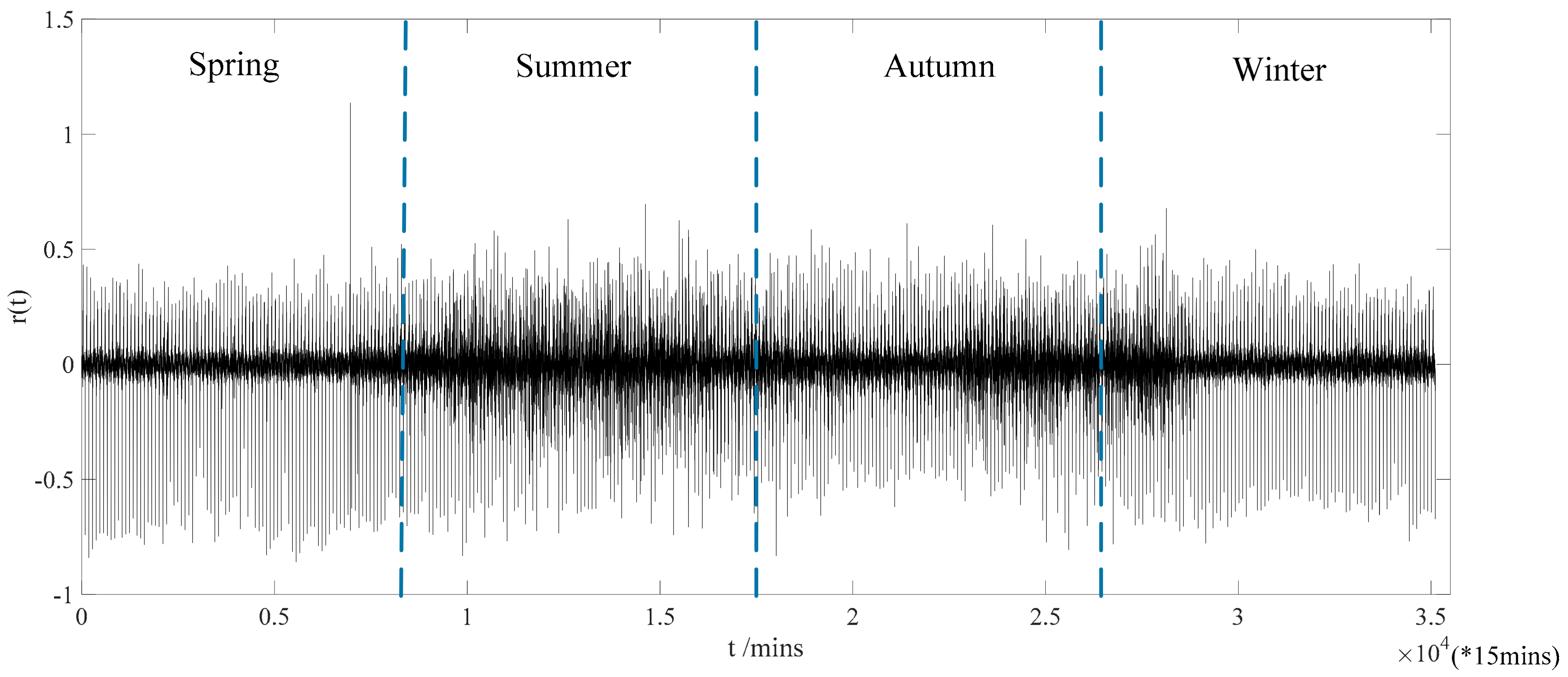
Figure 2.
Empirical and theoretical probability distribution of recurrence intervals between returns with different thresholds of power load for the office building.
Figure 2.
Empirical and theoretical probability distribution of recurrence intervals between returns with different thresholds of power load for the office building.

Figure 3.
Scaled probability distributions of recurrence intervals for different thresholds of power load in the office building.
Figure 3.
Scaled probability distributions of recurrence intervals for different thresholds of power load in the office building.

Figure 4.
Conditional probability density functions with (filled symbols) and (open symbols) for the office building.
Figure 4.
Conditional probability density functions with (filled symbols) and (open symbols) for the office building.
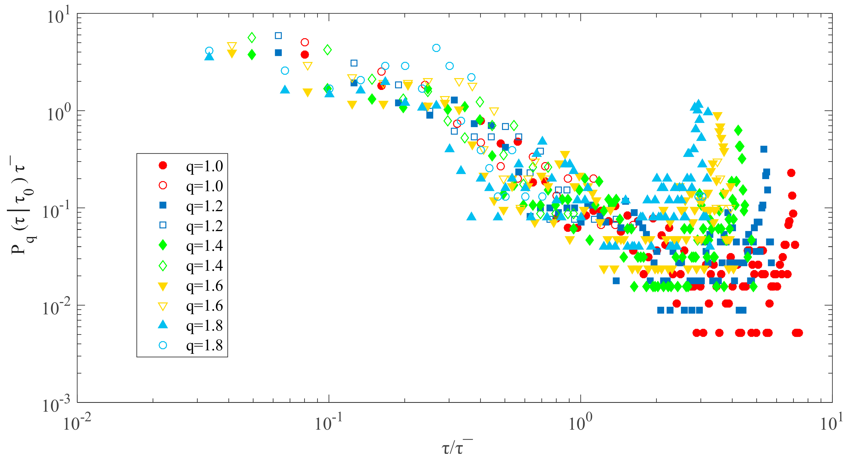
Figure 5.
Multifractal detrended fluctuation analysis (MF-DFA) of the office building in different thresholds. (a) Results of MF-DFA when ; (b) Results of MF-DFA when ; (c) Results of MF-DFA when; (d) Results of MF-DFA when; (e) Results of MF-DFA when .
Figure 5.
Multifractal detrended fluctuation analysis (MF-DFA) of the office building in different thresholds. (a) Results of MF-DFA when ; (b) Results of MF-DFA when ; (c) Results of MF-DFA when; (d) Results of MF-DFA when; (e) Results of MF-DFA when .

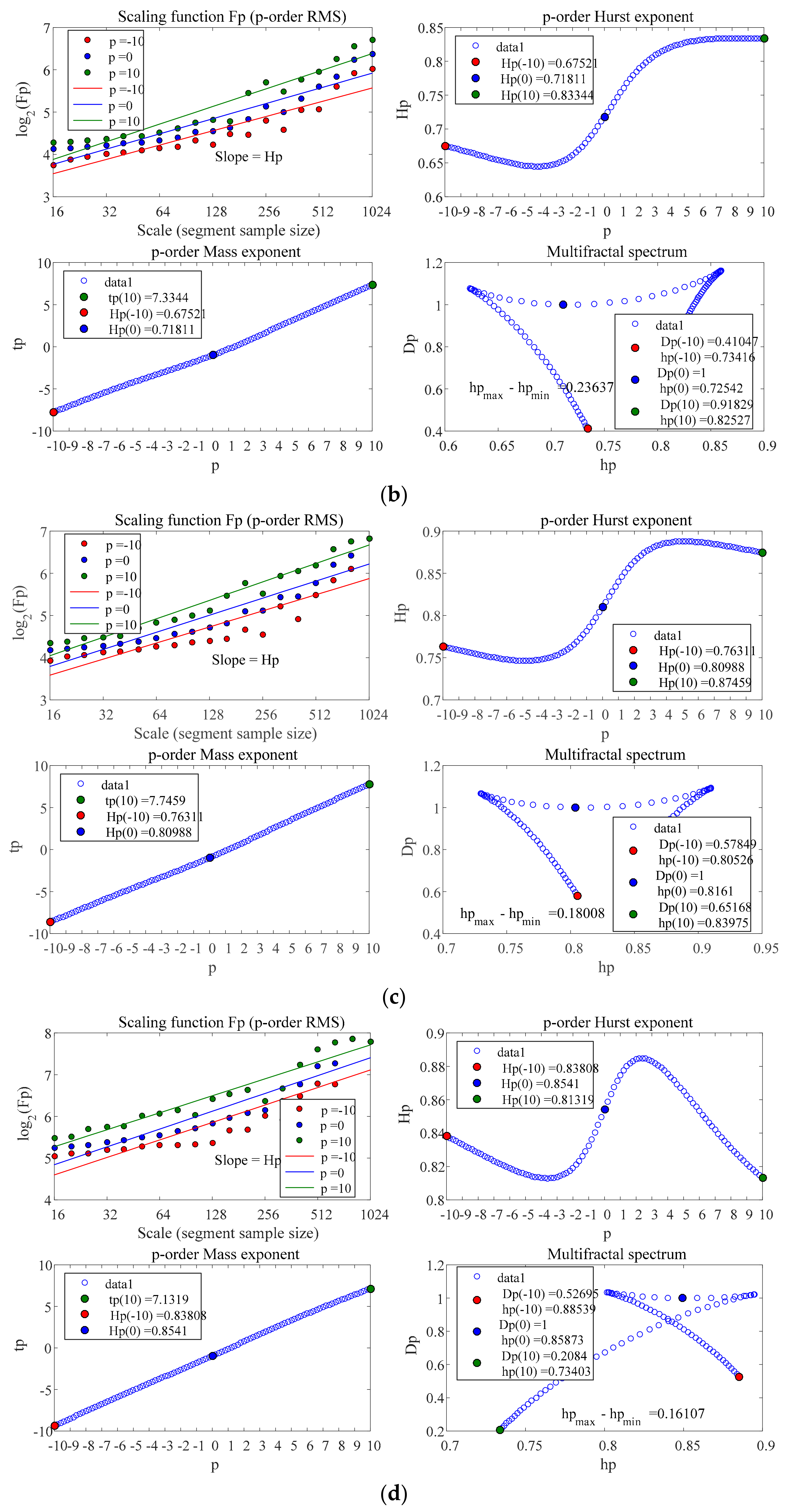
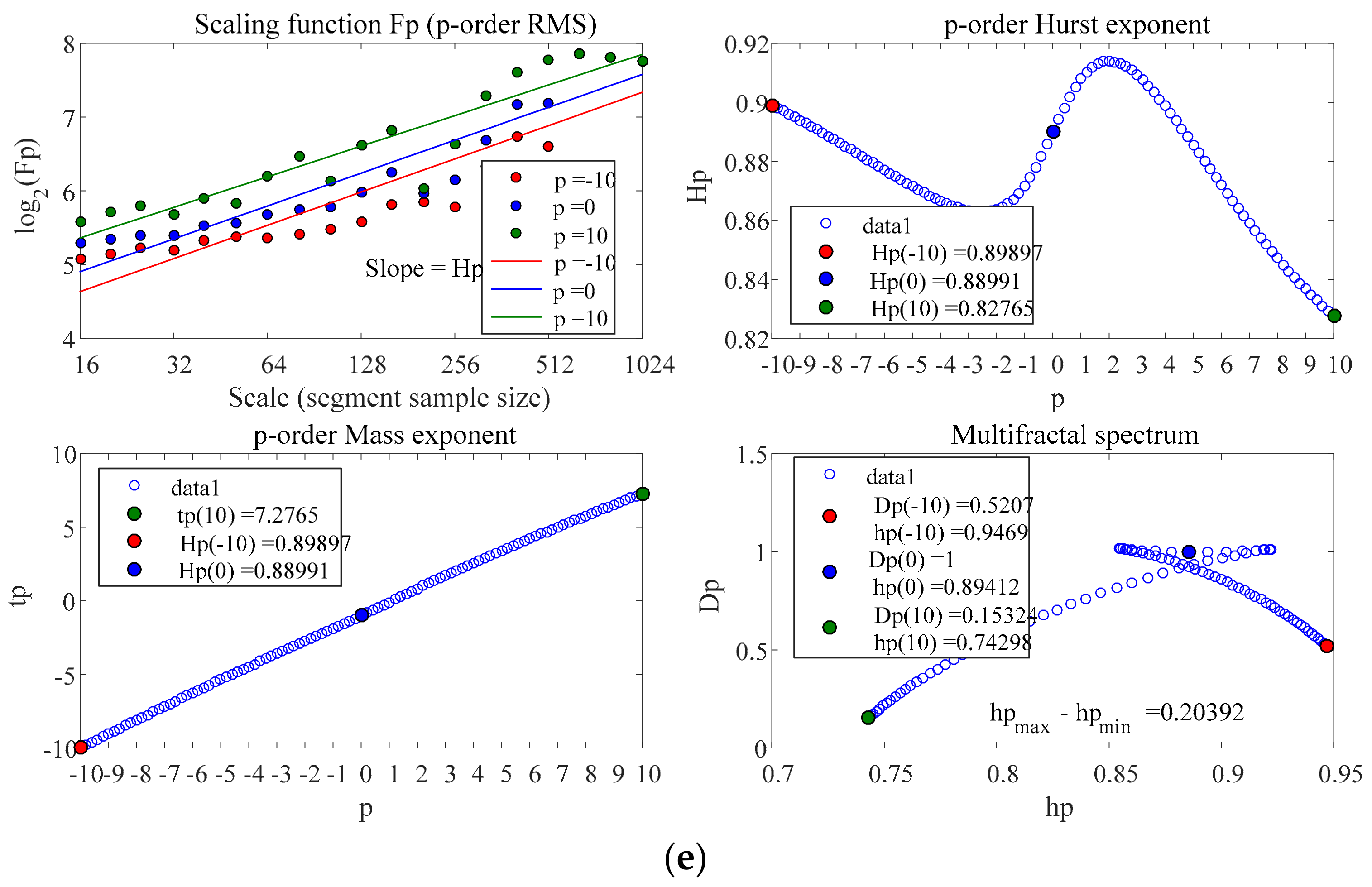
Figure 6.
Theoretical (curves) and empirical (color symbols) value of (x-axes are t, y-axes are values of for from top to bottom). (a) Empirical values and the curves are the theoretical values of for ; (b) Empirical values and the curves are the theoretical values of for ; (c) Empirical values and the curves are the theoretical values of for ; (d) Empirical values and the curves are the theoretical values of for ; (e) Empirical values and the curves are the theoretical values of for .
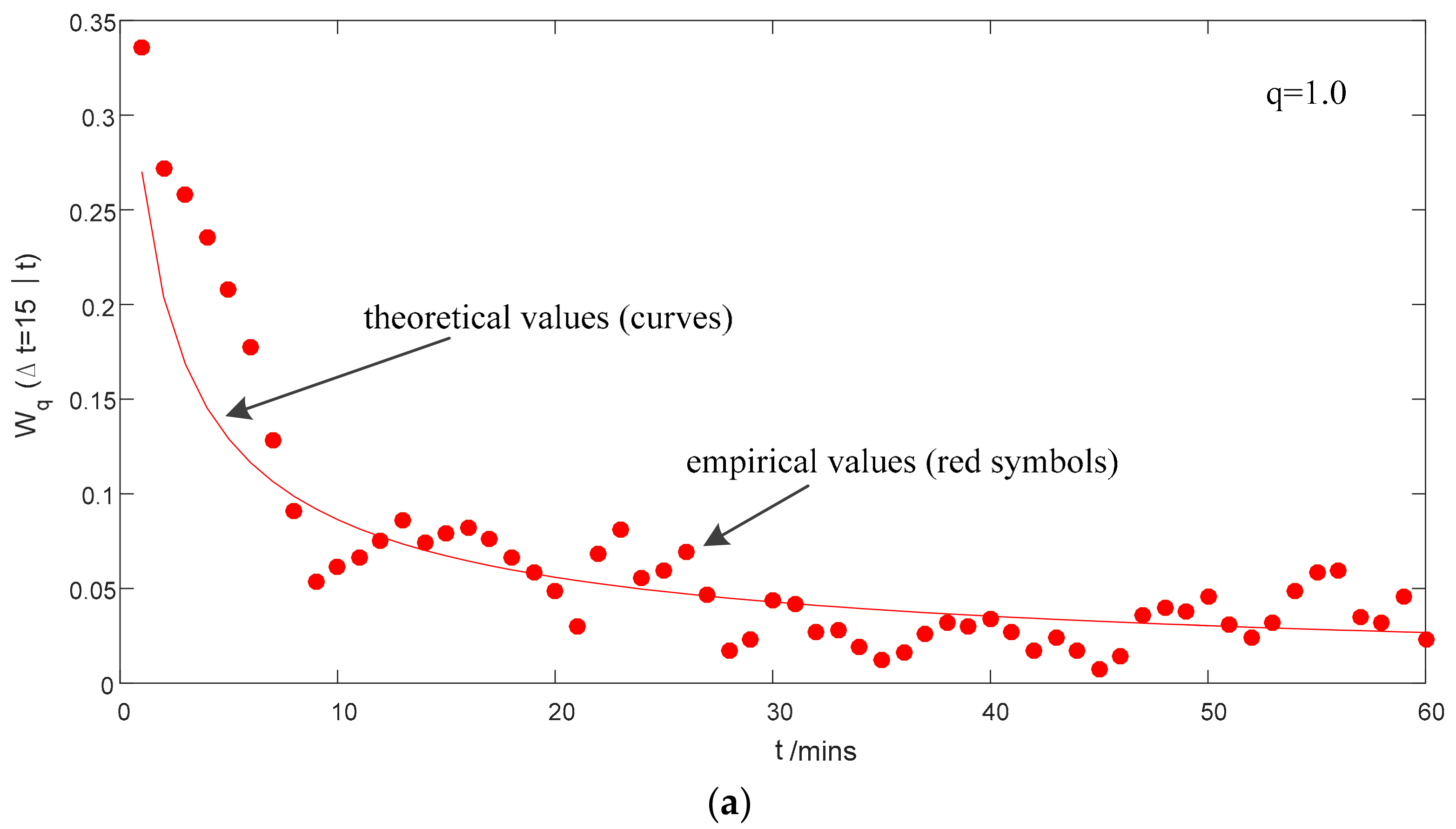
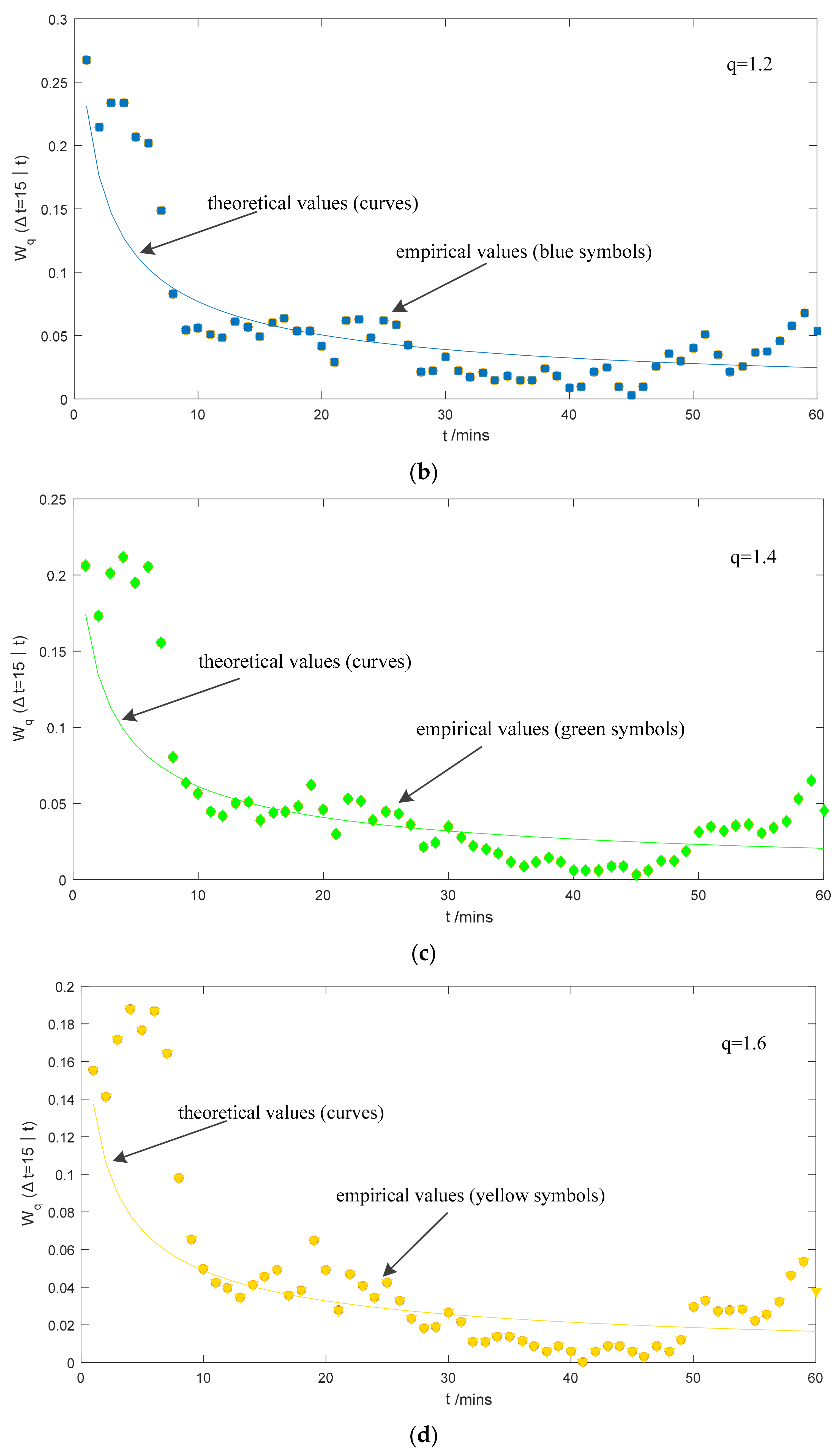

Figure 7.
The reciprocal of mean recurrence interval as a function of threshold.


Table 1.
Statistics of the returns of power load in the office building.
| Average | Maximum | Minimum | Standard Deviations | Skewness | Kurtosis | Nobs |
|---|---|---|---|---|---|---|
| 2.4240 × 10⁻⁵ | 1.1364 | −0.8591 | 0.1055 | −1.4120 | 17.5124 | 35,110 |
Table 2.
Estimates of the coefficients of stretched exponential functions.
| 1.0 | 2.228 | 89.399 | 0.2151 |
| 1.2 | 0.720 | 23.148 | 0.2269 |
| 1.4 | 0.207 | 5.756 | 0.2363 |
| 1.6 | 0.120 | 4.660 | 0.2260 |
| 1.8 | 0.025 | 0.338 | 0.2720 |
© 2018 by the authors. Licensee MDPI, Basel, Switzerland. This article is an open access article distributed under the terms and conditions of the Creative Commons Attribution (CC BY) license (http://creativecommons.org/licenses/by/4.0/).
Share and Cite
MDPI and ACS Style
Hong, L.; Shu, W.; Chao, A.C. Recurrence Interval Analysis on Electricity Consumption of an Office Building in China. Sustainability 2018, 10, 306. https://doi.org/10.3390/su10020306
AMA Style
Hong L, Shu W, Chao AC. Recurrence Interval Analysis on Electricity Consumption of an Office Building in China. Sustainability. 2018; 10(2):306. https://doi.org/10.3390/su10020306
Chicago/Turabian StyleHong, Lucheng, Wantao Shu, and Angela C. Chao. 2018. "Recurrence Interval Analysis on Electricity Consumption of an Office Building in China" Sustainability 10, no. 2: 306. https://doi.org/10.3390/su10020306
Note that from the first issue of 2016, this journal uses article numbers instead of page numbers. See further details here.