Comparison of Modeling Grassland Degradation with and without Considering Localized Spatial Associations in Vegetation Changing Patterns

Abstract

Grassland ecosystems worldwide are confronted with degradation. It is of great importance to understand long-term trajectory patterns of grassland vegetation by advanced analytical models. This study proposes a new approach called a binary logistic regression model with neighborhood interactions, or BLR-NIs, which is based on binary logistic regression (BLR), but fully considers the spatio-temporally localized spatial associations or characterization of neighborhood interactions (NIs) in the patterns of grassland vegetation. The BLR-NIs model was applied to a modeled vegetation degradation of grasslands in the Xilin river basin, Inner Mongolia, China. Residual trend analysis on the normalized difference vegetation index (RESTREND-NDVI), which excluded the climatic impact on vegetation dynamics, was adopted as a preprocessing step to derive three human-induced trajectory patterns (vegetation degradation, vegetation recovery, and no significant change in vegetation) during two consecutive periods, T₁ (2000–2008) and T₂ (2007–2015). Human activities, including livestock grazing intensity and transportation accessibility measured by road network density, were included as explanatory variables for vegetation degradation, which was defined for locations if vegetation recovery or no significant change in vegetation in T₁ and vegetation degradation in T₂ were observed. Our work compared the results of BLR-NIs and the traditional BLR model that did not consider NIs. The study showed that: (1) both grazing intensity and road density had a positive correlation to vegetation degradation based on the traditional BLR model; (2) only road density was found to positively correlate to vegetation degradation by the BLR-NIs model; NIs appeared to be critical factors to predict vegetation degradation; and (3) including NIs in the BLR model improved the model performance substantially. The study provided evidence for the importance of including localized spatial associations between the trajectory patterns for mapping vegetation degradation, which has practical implications for designing management policies to counterpart grassland degradation in arid and semi-arid areas.

1. Introduction

Grasslands are the most widely distributed natural ecosystems, and play a vital role in global carbon recycling, as well as serve as an important livestock husbandry base for agricultural activities [1,2]. Grassland degradation has attracted wide attention worldwide. Grassland covers more than 40% of China’s total land area, a large percentage of which is found in the Inner Mongolia Autonomous Region (IMAR) [3]. Due to arid and semi-arid climate conditions, as well as the impact of human activities during the past several decades, the grassland ecosystems showed a limited capacity to withstand human interference; as a result, grassland degradation has been widely observed in IMAR [4,5,6]. Grassland degradation is a complex process in which grassland productivity, vegetation coverage, grass height, soil biodiversity, or community composition decreases [7,8,9,10]. Numerous studies focusing on the characteristics, processes, and mechanisms of grassland degradation and on the restoration of degraded vegetation have been conducted [1,7]. Development in remote sensing technology in the past few decades has significantly advanced the work in vegetation cover monitoring [11,12,13,14,15]. Huge datasets were accumulated by remote sensing sensors, which greatly facilitated studies in grassland ecosystems. Based on the integration of remotely sensing data and other socio-economic data, a few important issues related to grassland degradation were analyzed. For example, steppe degradation in arid and semi-arid areas could be the result of both climate conditions, particularly due to limited precipitation, and intensified human activities [16,17]. Furthermore, studies on the driving factors of grassland degradation, both natural and human-induced, presented some critical insights for understanding the pathways of vegetation deterioration and their mechanisms [18,19]. Typical examples of natural driving factors included climatic conditions, local environments (e.g., topography such as elevation, slope, or aspect), and soil properties [20,21,22]. Some human-induced factors, including overpopulation, overgrazing from livestock, and transportation, were also identified as being threatening factors for the grassland ecosystem [23,24,25,26]. Intensified human disturbance due to increased accessibility to remote regions, as a result of the construction of more road networks, have led to vegetation degradation in many parts of the world [17,27,28,29].

While the constraints from natural factors are difficult to remove, threats from human-induced factors are relatively easier to alleviate by means of designing more sound land use policies, e.g., rotational grazing, fenced grazing, or through vegetation recovery projects [30]. Therefore, quantifying vegetation degradation due to human-induced factors attracted much attention from grassland policymakers and experts in academia [31,32]. Evans and Geerken proposed a method called residual trend analysis, or simply RESTREND, to discriminate the roles on dryland degradation played from climatic and human-induced factors based on the residuals of regression between the normalized difference vegetation index (NDVI) and precipitation [33]. RESTREND has since been applied widely to explore the associations between grassland degradation and human-induced vegetation changes [31,34,35,36,37].

Remote sensing and spatial analysis can be combined to map the trajectory patterns (TPs) of grassland vegetation based on historical time-series data. It is of great value to understand the factors that explain TPs, and preferably, to predict future vegetation degradation. However, land use change is a complex process that is not easy to model [38,39,40]. Pattern based land-use models have been widely applied to map land-use changes [41]. Relying on observations from a list of potential driving variables, pattern based land-use models were implemented to quantify the relationships of land-use patterns and those variables of interest [42]. In addition, localized spatial associations, or neighborhood interactions contained in the land use patterns, have proved to be helpful in studying land use changes [43]. Cellular automata, usually referred to as a CA model, is a typical example that uses the links or characteristics of neighborhood interactions in land use patterns to model the dynamics of land use expansion [44]. Neighborhood interactions (NIs) reveal the degree of dependence between TPs in a local space, which are usually defined by a neighborhood matrix, and NIs could be important factors for determining further directions of TPs [45]. By characterizing neighborhood interactions, global as well as spatially varied, or localized associations between different TPs were measured [46]. There have been a few methods proposed for quantifying such neighborhood interactions. For example, Verburg et al. [46] proposed an index called the enrichment factor (F); for every location defined in a grid dataset, the characteristics of interactions between land cover types could be measured. In the case of modeling grassland degradation, NIs, implying possible spatial interactions between TPs, might also be helpful.

The primary aim of this paper is to validate the effectiveness of including NIs along with other human-induced driving factors in modeling grassland vegetation degradation. Binary logistic regression (BLR) has been widely applied to studying cause–effect relationships. BLR is capable of predicting the odds of being a case or not (responses from a binary variable) based on the values of the independent variables (predictors), and thus is fit for studying vegetation degradation [18]. We compared two models based on binary logistic regression: the traditional binary logistic regression model (simply referred to as BLR hereafter), and a binary logistic regression model with neighborhood interactions (referred to as BLR-NIs). With the support of historical data, it is possible to predict the probability of future vegetation degradation by the BLR models.

2. Study Area, Data Sources and Methodology

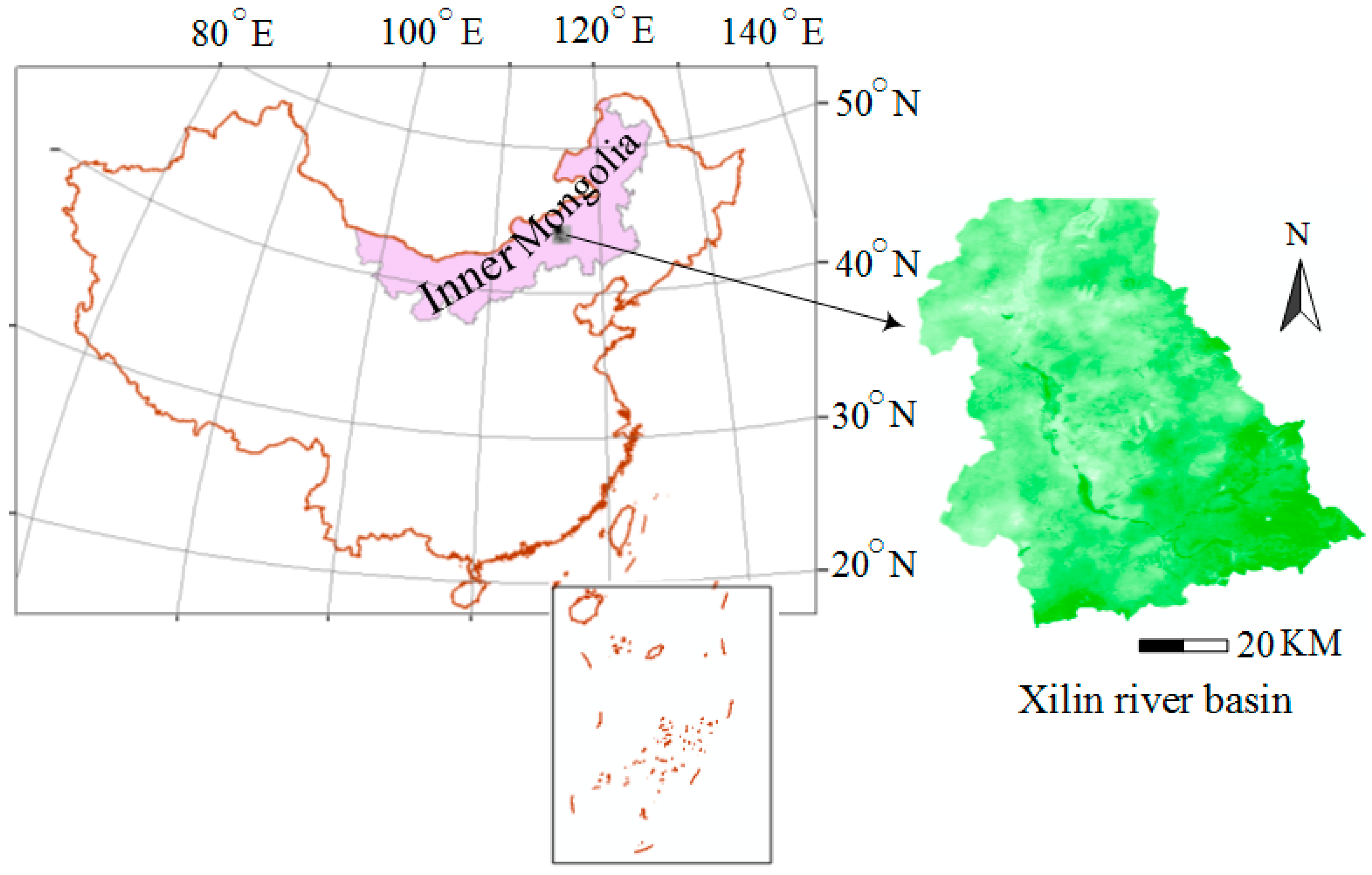
2.1. Study Area

The study area was in the Xilin river basin located between 43°26′ and 44°29′ North and 115°32′ and 117°12′ East in the Inner Mongolia Autonomous Region (IMAR), China (Figure 1). It is one of the most representative steppe zones in China. Out of the total area about 10,000 km², approximately 90% of the region is covered by grassland [44]. The area belongs to the continental semi-arid grasslands of the central Asian steppe ecosystem [47]. The annual mean temperature of the area ranges from 1 °C to 4 °C [48], while annual mean precipitation is about 350 mm, most of which concentrates between June and August [49]. Needle grass (scientifically known as Stipa grandis) and false wheatgrass (Leymus chinensis) are two dominant species in the area [50], and dominant soil types include chestnut, chernozem, and Aeolian [51]. The growing season (from May to September) of local plants usually starts in late April and ends in late September. Agriculture is the primary income for the local people. Breeding livestock on the grassland is one of the most important activities for the farmers. Fenced grazing and rotational grazing were adopted since the early 2000s in some parts of the region to avoid overgrazing from the grassland animals.

2.2. Data Sources

In order to study the vegetation degradation in relationship to human activities (including grazing intensity and road network density), we acquired NDVI data, climatic data, grazing intensity data, and road network data. The NDVI data were obtained from the NASA MODIS MOD13Q1 vegetation index dataset for the years 2000–2015. MOD13Q1 were provided every 16 days at 250-meter spatial resolution. Maximum annual NDVI (NDVI_max) was computed and represented the annual climax productivity of the grassland vegetation. The climatic data were obtained from China’s Meteorological Data Sharing Service System (http://cdc.cma.gov.cn), which included monthly precipitation data collected from 680 weather stations across the entire country. Ordinary Kriging spatial interpolation was adopted to generate monthly precipitation thematic maps, considering its capability of giving unbiased predictions with minimum variance for the target variable. Grazing intensity (GI) was one of the most representative human-induced factors that caused grassland degradation. GI data were collected from the local statistical yearbook during the study period. There were five recorded animal species, that is, sheep, horse, buffalo, camel, and donkey. Since different livestock have varied impacts on grass consumption and vegetation damage, each of the livestock was converted to a standard animal unit, called a sheep unit, through a conversion coefficient to compute the grazing intensity [18]. By converting all of the animal species to sheep unit, it is more convenient to model the overall grazing effect. Local farmers helped determine the coefficients, which represented the magnitude of grass consumption and vegetation damage from a particular animal type relative to that from one sheep, through a questionnaire survey. Specifically, one horse is equivalent to six sheep, and thus was multiplied by six to transform into the sheep unit. Similarly, cattle, camel, and donkey were multiplied by five, seven, and three, respectively. The road network was collected from an open source project called Open Street Map (OSM), as well as traffic road maps from the local transportation bureau. The line density analysis from the ArcGIS Spatial Analyst toolbox was used to compute road density (RD) for both OSM and the traffic road map, separately. Then, the two RD maps were overlaid to get the maximum value as RD. In the end, all of the dataset were resampled to 250 m × 250 m, and clipped using the boundary of the study region.

2.3. Methodology

The NDVI-based residual trend (RESTREND-NDVI) method proposed by Evans and Geerken [33] was used to extract human-induced grassland degradation for two consecutive periods, T₁ (2000–2008) and T₂ (2007–2015), respectively. Here, the purpose of designing two periods was to test the power of predicting patterns of vegetation change for the next stage (namely T₂) based on the previous stage (T₁), because vegetation change not only depends on spatial context, but also presents time-lag, which indicates the linkage of patterns of vegetation change in a temporal context. NDVI has a significant positive correlation with rainfall in arid and semi-arid drylands [34]. By performing regression analysis between precipitation data and annual NDVI_max at the pixel level, the associated residuals in each period could be mapped in a linear regression [33]. A positive trend in residuals indicates an increasing NDVI signal relative to precipitation, i.e., vegetation recovery (RR), whereas a negative trend in residuals indicates a declining NDVI signal relative to precipitation, i.e., vegetation degradation (DD); if the residuals show no significant trend, then no significant change (NS) in vegetation is detected [33,34,52].

Based on the above patterns (RR, DD, or NS) of vegetation change identified for each period (T₁ and T₂), vegetation degradation (VD) was redefined based on the conversions matrix of TPs from T₁ to T₂: if RR or NS was observed in T₁ and DD was observed in T₂, suggesting significant decreased vegetation productivity in T₂ compared with that in T₁. This definition emphasized the changes of TPs in two consecutive periods, and this conversion was attributed to human activities. Similarly, vegetation restoration (VR) was redefined for the cases when DD or NS was present in T₁ and RR observed in T₂, indicating an improvement of vegetation productivity in T₂.

The time-lag effect may influence patterns of vegetation change, and the characterization of neighborhood interactions was computed by Verburg’s F index [46], which measures the localized impact of each pattern (RR, DD, or NS) on vegetation degradation in a local region relative to that in a whole study area. As there were three involved patterns, namely RR, DD, and NS, which were derived from the vegetation dynamics based on the historical NDVI and precipitation data, three F_i,k,d variables corresponding to pattern k (k = RR, DD, or NS) at each pixel (location) i within a local window defined by a predefined size d were computed for period T₁. The average neighborhood characteristic for a particular pattern k can be calculated by taking the average F for all pixels. We were interested in testing whether the neighborhood interactions at an earlier period (T₁) given by the three F indices helped to predict vegetation degradation. The parameter d was relatively difficult to determine. Verburg et al. [46] found that the average neighborhood characteristic for a land use type changed from other land use types, and varied with different window sizes, but usually leveled off after a threshold. We found that the average neighborhood characteristic for DD developed from RR and NS showed a negligible change to window size when it was beyond seven units. Considering this result, as well as the previous study on vegetation density interpolation [18], d was set to seven (equivalent to a window with 1.75 km in width).

Binary logistic regression (BLR) is a bivariate statistical analysis model that predicts the probability of a binary response, for example, the presence or absence of an event. The BLR model provides insights into the relationship between a dependent variable, and one or a set of independent explanatory variables. Formally, the probability of occurring vegetation degradation (y) is a function for a vector X(x₁, x₂, …, x_n):

$$\ln \left(\frac{\mathrm{P}\left(\mathrm{y}=1|\mathrm{X}\right)}{\mathrm{P}\left(\mathrm{y}=0|\mathrm{X}\right)}\right)=\ln \left(\frac{\mathrm{P}\left(\mathrm{y}=1|\mathrm{X}\right)}{1-\mathrm{P}\left(\mathrm{y}=1|\mathrm{X}\right)}\right)={\mathsf{\beta }}_0+{{\displaystyle \sum }}_{\mathrm{i}=1}^{\mathrm{n}}{\mathsf{\beta }}_{\mathrm{i}}{\mathrm{x}}_{\mathrm{i}}$$

(1)

where y is a binary variable that takes 1 as meaning an occurrence of vegetation degradation, or 0 as meaning the opposite; $\mathrm{P}\left(\mathrm{y}=1|\mathrm{X}\right)$ denotes the probability that the event occurred at a certain location; element x_i (i = 1, 2, …, n) in X corresponds variable i explaining y, $\mathrm{P}\left(\mathrm{y}=1|\mathrm{X}\right)$/$1-\mathrm{P}\left(\mathrm{y}=1|\mathrm{X}\right)$ is the odds ratio, and ln$(\mathrm{P}\left(\mathrm{y}=1|\mathrm{X}\right)$/$\left(1-\mathrm{P}\left(\mathrm{y}=1|\mathrm{X}\right)\right))$ is a logit transformation. β₀ and β_i (i = 1, 2, …, n) are the regression coefficients of the function, which are best fit by a maximum likelihood estimation algorithm.

Climate impact was excluded from being a contributing factor, since the vegetation degradation was derived by the RESTREND-NDVI method. Therefore, explanatory variables from human activities, including RD and GI, were taken in the BLR analysis, while the post-processed vegetation degradation (VD) was taken as the dependent variable. The RD and GI in T₂ were temporally averaged and input to the BLR models. In addition, neighborhood interactions (NIs) are also possible factors. It is of great value to know whether including NIs in the patterns of vegetation change improves the performance of vegetation degradation modeling. To examine the contribution of NIs, two BLR models—BLR-NIs that considered NIs and the other that did not (simply BLR)—were built and compared. All of the explanatory variables were standardized into zero-mean, following the formula:

$${\mathrm{x}}_{\mathrm{i}}^{*}=\frac{{\mathrm{x}}_{\mathrm{i}}-\overline{\mathrm{x}}}{\mathsf{\sigma }}$$

(2)

where ${\mathrm{x}}_{\mathrm{i}}^{*}$ denotes the standardized value of variable x for sample/location i, ${\mathrm{x}}_{\mathrm{i}}$ is the original value of the variable, $\overline{\mathrm{x}}$ is the mean value, and $\mathsf{\sigma }$ is the standard deviation of the original variable. After substituting x_i with ${\mathrm{x}}_{\mathrm{i}}^{*}$ in Equation (1), the result of the regression can be expressed in terms of conditional probability at any spatial location (pixel i) to be predicted:

$$p_{\mathrm{i}}=\frac{\exp \left({\mathsf{\beta }}_0+{{\displaystyle \sum }}_{\mathrm{i}=1}^{\mathrm{n}}{\mathsf{\beta }}_{\mathrm{i}}{\mathrm{x}}_{\mathrm{i}}\right)}{\left(1+\exp \left({\mathsf{\beta }}_0+{{\displaystyle \sum }}_{\mathrm{i}=1}^{\mathrm{n}}{\mathsf{\beta }}_{\mathrm{i}}{\mathrm{x}}_{\mathrm{i}}\right)\right)}$$

(3)

The probability of vegetation degradation (VD) at a location i, indicated by p_i, in the study region could be calculated according to Equation (3). It is a straightforward computation to make a probability map of vegetation degradation over a given region when the required data for the models (BLR and BLR-NIs) are available.

A total of 6.5% of pixels labeled with VD and non-VD were randomly selected from the processed dataset and split into two parts with equal size (5000 samples) to fit and test the BLR and BLR-NIs, respectively. A confusion matrix and relative operating characteristic (ROC) were adopted to evaluate the performance of the models [53]. The confusion matrix method uses a contingency table (also known as a cross-tabulation) to display a multivariate frequency distribution of the variables, and evaluate the classification accuracy of the models. The ROC method is based on a curve relating the true-positive rate and the false-positive rate over a range of cutoff values in classifying the probability. The area under the curve (AUC) is used to evaluate the accuracy of the model. The AUC varies between 0.5 (completely random) and 1 (perfect discrimination), and values above 0.7 are generally assumed to indicate a good model fit [54]. All of the statistics were performed using the Statistical Package for the Social Sciences (SPSS, v22).

3. Results

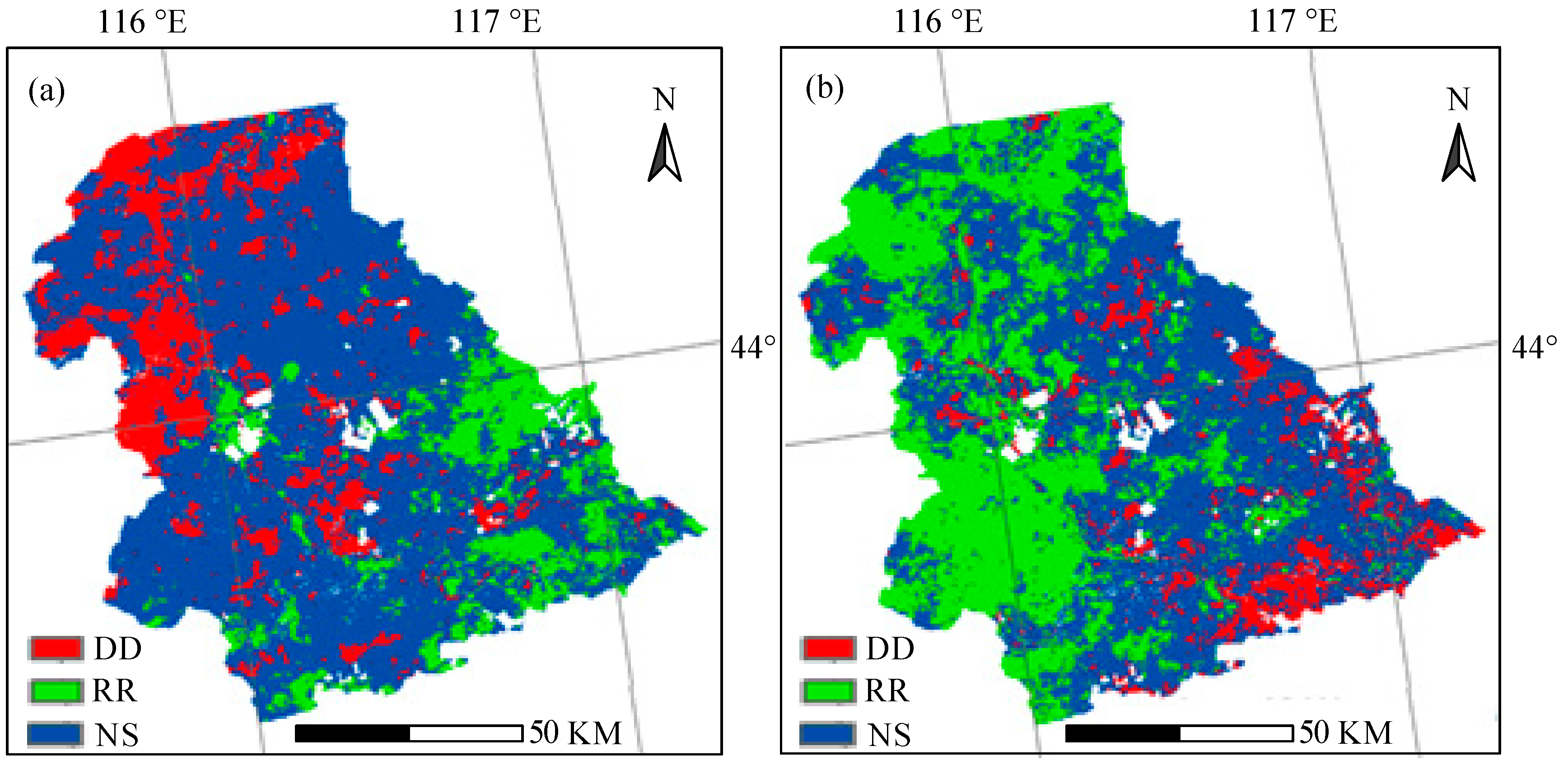
3.1. Spatio-Temporal Patterns in Vegetation Change

While a great part of area showed no obvious change (NS) in vegetation cover for both T₁ and T₂, a significant difference was observed in the spatial distribution of RR and DD between period T₁ and T₂ (Figure 2). The DD during T₁ was mostly observed in the northwestern part (covering 16.75% of the total area), and RR mainly dominated the southeastern part, covering 12.80% of the total study area. Conversely, during T₂, DD mainly appeared in southeastern region, which only took 8.64% of the total area, but RR shifted to the northwestern part, which showed a much larger area (36.29%) when compared with that in its previous period. Furthermore, a great part of the area in the southwest was also categorized as RR during T₂.

The patterns of vegetation change present in each of the two periods (T₁ and T₂) exhibited much spatial variation. After the patterns in T₁ and T₂ were overlaid, several combinations were obtained. There was a clear spatial shift in the distribution of the patterns between the two study periods. For example, locations that showed stable (NS) or even recovered (RR) in vegetation productivity at an earlier stage (T₁), but significantly declined (denoted as DD) at a later stage (T₂), were mostly located in the southeastern part of the study area (Figure 2). Conversely, most of the degraded (DD) or no significant (NS) change in vegetation cover at T₁ appeared to recover (RR) at a later stage (Figure 2). This spatial shift in the distribution of the patterns in vegetation change indicated a revertible trend in vegetation changes. The result from the overlaying the layers of the patterns of vegetation change indicated a relatively small percentage of vegetation degradation compared to that of vegetation recovery (7.71% for VD vs. 34.78% for VR, in Figure 3).

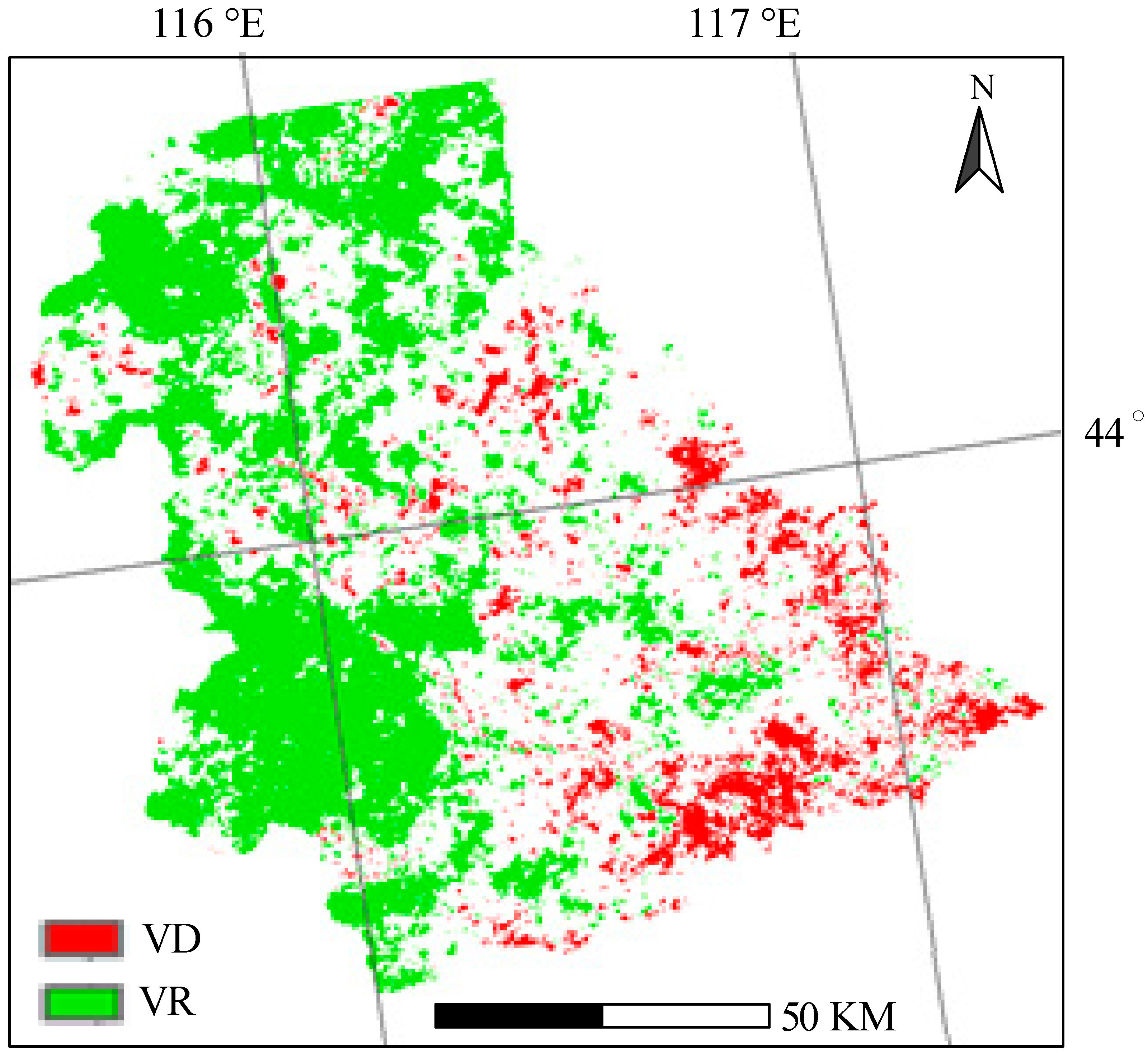
3.2. Comparison of Vegetation Degradation by the BLR Models

The modeling results for vegetation degradation by the BLR—with and without NIs—are listed in

Table 1. Results of two binary logistic regression (BLR) models.

Model	Variable	β	Exp(β)	95% CI for Exp(β)
				Lower	Upper
BLR	GI	0.610	1.841	1.554	2.180
	RD	1.847	6.339	5.634	7.133
	Const.	0.417	1.518
BLR-NIs	#GI
	RD	1.671	5.318	4.673	6.052
	FDD	−0.749	0.473	0.413	0.541
	FRR	2.176	8.812	6.820	11.387
	#FNS
	Const.	0.832	2.299

CI: confidence intervals; Exp(β): odd ratio; #variables not significant in the model (α = 0.01); the cut value is 0.5.

. The BLR model demonstrated that grazing intensity and road density were significant and positive contributors to the human-induced vegetation degradation. For grazing intensity, the odds ratio Exp(β) could be interpreted as an increase of grazing intensity by one standardized unit almost doubling the possibility of human-induced degradation (184.1%). Road density exhibited an even more significant impact on the predicted probability of grassland degradation. When road density increased by one standardized unit, the probability for vegetation degradation increased more than six times (i.e., 6.339).

When the localized association variables, or neighborhood interactions (NIs) in TPs, were added to the BLR model (BLR-NIs), some changes were observed. First, grazing intensity was excluded from the model, demonstrating that the impact of grazing intensity was diminished (from significant in the BLR to insignificant) with the inclusion of NIs. Road density in BLR-NIs was still significantly and positively correlated with grassland degradation, with the coefficient (β) reduced from 1.847 to 1.671, suggesting that a one unit increase in standardized road density would lead to a high probability (increased more than five times) of vegetation degradation. Though the neighborhood interactions (DD, RR, and NS) in TPs demonstrated their impact on vegetation degradation, they presented different roles. For example, a higher F value in RR (F_RR) would lead to a greater likelihood for vegetation degradation, meaning that the locations with RR at T₁ were much more likely to experience vegetation degradation in the next period. The VD probability with a unit increase in standardized F_RR would increase more than eight times (Exp(β) = 8.812). Conversely, a higher F value in DD (F_DD) would cut the probability in vegetation degradation in half (Exp(β) = 0.473) with a standardized unit increase. Lastly, the F value for NS (F_NS) did not show a significant impact on the vegetation degradation.

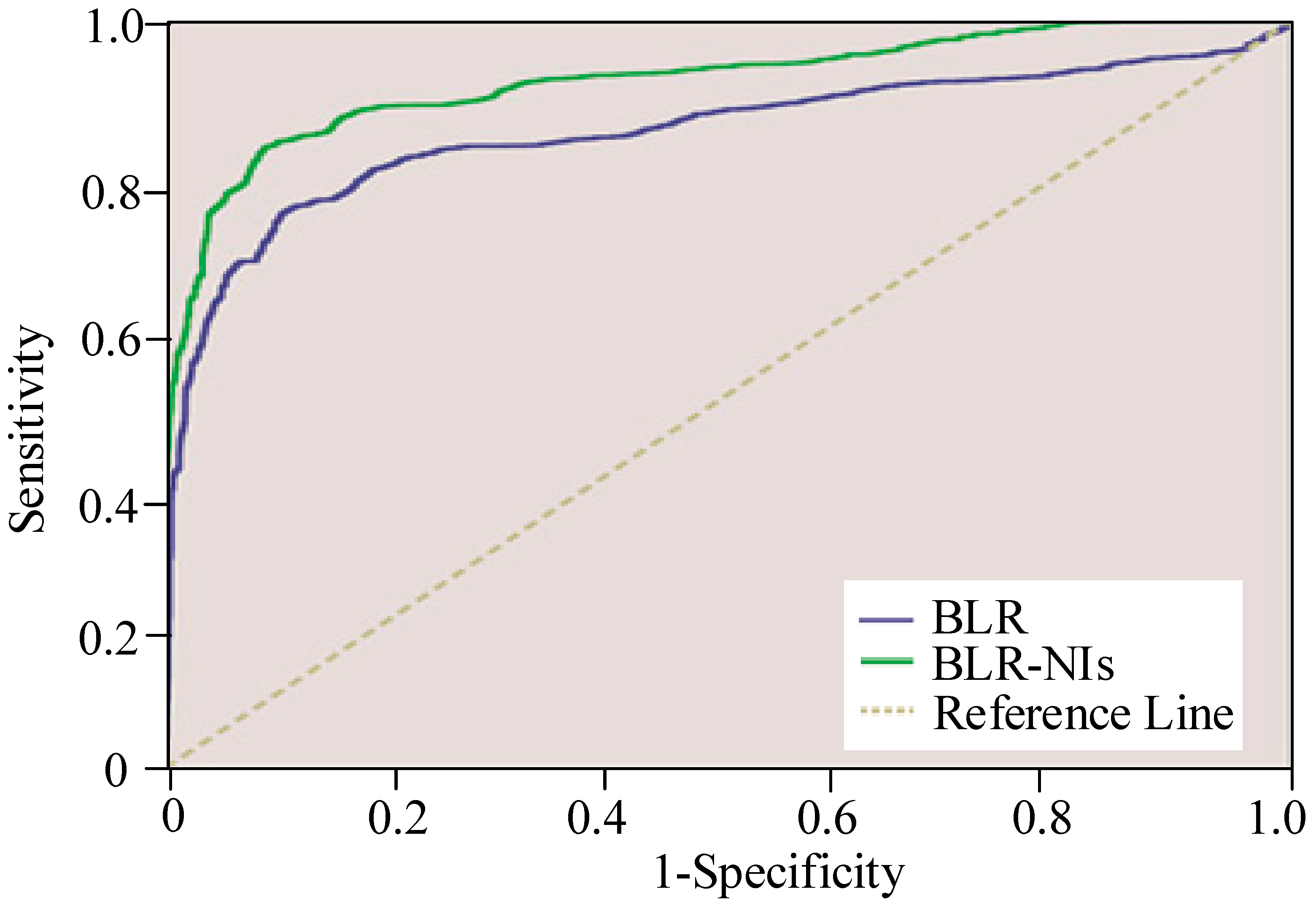
3.3. Accuracy Evaluation

Table 2. Classification table for two BLR models. VD: vegetation degradation.

Model	Data from	Response	Predicted		Percentage Corr.
			VD	Non-VD
BLR	Observed	VD	1701	799	68.0%
		Non-VD	205	2295	91.8%
		Overall acc.			79.9%
BLR-NIs	Observed	VD	1940	560	77.6%
		Non-VD	163	2337	93.5%
		Overall acc.			85.5%

presented the accuracy of the two models, comparing the results of the observed and predicted VD. The percentage correct for the positive case (VD) was 68.0% for the BLR model and 77.6% for the BLR-NIs model, while that for negative case (non-VD) was 91.8% and 93.5% for the BLR model and the BLR-NIs model, respectively, suggesting that both models had better prediction power for the negative cases. The overall accuracy for the BLR model and the BLR-NIs model was 79.9% and 85.5%, respectively. From the performance of both the percentage correct and overall accuracy, the BLR-NIs model showed improved power in predicting VD over the BLR model, indicating the importance of the inclusion of localized spatial associations in TPs.

The ROC curves for the two BLR models were compared. Figure 4 and

Table 3. Statistics of the pseudo R² and area under the curve (AUC) for BLR models with and without neighborhood interactions (NIs).

Model	Cox & Snell R2	Nagelkerke R2	AUC
BLR	0.368	0.490	0.850
BLR-NIs	0.499	0.665	0.919

show that the AUC for the BLR and BLR-NIs models was 0.850 and 0.919, confirming that the model BLR-NIs had a better accuracy than the BLR model in predicting the probability of vegetation degradation. Finally, pseudo Cox & Snell and Nagelkerke R², both computed as the ratio of the variance explained by independent variables to the total of the dependent, but from different aspects, for the two models are summarized in Table 3. For both R², the values for the BLR-NIs model were much higher than those for the BLR model, suggesting that the variables taken in the BLR-NIs model have more explanatory power.

4. Discussion

This paper tried to analyze human-induced grassland degradation through residual trend analysis on the normalized difference vegetation index (RESTREND-NDVI), which is often adopted for arid or semi-arid regions, and to quantify the degradation with two typical factors from human activities. Transportation (road density) and grazing (intensity) were selected in the study because they had been widely recognized as driving factors of vegetation productivity. Our emphasis on human-induced vegetation degradation was based on the consideration that they were relatively easier to be reduced through designing sound grassland management plans. Nevertheless, very few models accounted for the neighborhood interactions (NIs) in the patterns of vegetation change when studying grassland vegetation degradation. Here, we compared two binary logistic regression (BLR) models to explain the vegetation degradation. While both of them included the two human-induced factors, our initial hypothesis was that NIs could be important predictors, and might be able improve model performance.

Overgrazing has long been regarded as the principal factor driving vegetation degradation [8]. Previous studies also indicated that overgrazing has been present in the Xilin river basin for a long time, triggering a series of ecological problems, including serious grassland degradation [23,48,55]. This was also confirmed in the BLR model, which presented a significant and positive coefficient in the fit BLR function, suggesting that higher grazing intensity led to a greater likeliness of vegetation degradation. Under the influence of overgrazing, the structure, productivity, or biological characteristics of grassland vegetation could be affected [9,10]. Furthermore, overgrazing on vegetation often resulted in the degraded succession of vegetation communities, causing degradation in vegetation productivity in the end [56]. However, it is interesting that the grazing intensity was not listed as a significant contributor to vegetation degradation once the characteristics of neighborhood interactions were accounted for in the modified BLR model, i.e., the BLR-NIs model. This result indicated that the grazing effect could have been included and reflected in the characterization of the neighborhood interactions, which was captured by the F indices in the BLR-NIs model.

Compared to other factors, road accessibility showed the strongest impact on vegetation degradation. The significance was confirmed by both of the BLR models. While constructing more road networks expanded the domain of human activities, it also might lead to more damage to the grassland vegetation due to the easier access to vegetated areas. The side impact on vegetation due to road networks on grasslands has been documented by a few studies investigated in Inner Mongolia and Mongolia [18,57]. The paper [57] also analyzed a few reasons, including the hardness of the top layer and soil erosion, for the damage imposed by road tracks on grasslands. The BLR models in the current study suggest that a one-unit increase in the standardized road network density led to a five to six-fold increase in the probability of vegetation degradation. Traditionally, local people relied more on fixed locations for livestock grazing; in the last few decades, more and more road networks were built with the economic development of the region, which greatly facilitated moving grazing and the formation of more village centers in the countryside [18]. The current study indicated that the grassland vegetation adjacent to the road network was more likely to suffer degradation.

Many factors, ranging from human activities to climate change, have proved to be important for grassland vegetation dynamics. However, previous studies rarely consider how neighborhood interactions impact vegetation degradation. In fact, vegetation degradation is not only affected by exterior factors (e.g., precipitation or grazing), it also varies under different spatial and temporal contexts of the patterns of vegetation change. For example, in our previous study, from the perspective of vegetation succession patterns, we found that grassland degradation was closely related to the background vegetation types from which the successions developed [18]. This study revealed that vegetation degradation was more likely to occur at places where vegetation showed a recovery pattern (denoted as RR) at an earlier time, but was less likely to happen if vegetation had already showed degradation (labeled as a DD pattern) previously in the BLR-NIs model. This finding suggests that the patterns of vegetation change in the study region tended to reverse/convert over time, making it necessary to continue to enforce vegetation protection policies in the already recovered vegetated area, while at the same time strengthening efforts to improve other degraded areas. Out of those policies, an adaptive grazing strategy has been introduced in the past decade to allow grassland pasture to be fed by livestock in a rotational manner, which prohibits continuous grazing at the same location, and instead encourages feeding livestock at different locations based on the availability of pasture. Adaptive grazing tends to balance grazing intensity over an entire region by interrupting grazing always in degraded (DD) areas, and looking for vegetation recovered (RR) areas or areas with no significant (NS) change in vegetation. Other enforced strategies such as fenced grazing also prevented grassland vegetation from severe degradation [4]. Similar outcomes resulted from the enforcement of those policies (e.g., adaptive grazing) may suggest certain clues for the insignificance of the grazing effect once the neighborhood interactions in TPs were included in the model.

Regression analysis is a typical method for estimating the relationships among variables. Binary logistic regression analysis is based on a regression model particularly fit for investigating the dependence of a variable with two responses, one positive and one negative, on a set of explanatory variables. Understanding the probability of the occurrence (or non-occurrence) of vegetation degradation is very important for the sustainable development of the grassland ecosystem. It is reasonable to apply BLR-based models to investigate factors related to grassland degradation. With support from available statistical packages such as SPSS, BLR models could be quickly fit and evaluated. The two BLR models (BLR versus BLR-NIs) compared the results between including and excluding neighborhood interactions in the prediction of the probability of vegetation degradation. Compared with the BLR model, the BLR-NIs model had much improvement in the prediction power. The outcome from the BLR models, particularly the odd ratio (i.e., Exp(β)) provided a valuable reference for policymakers in regard to designing informed strategies for improving grassland management in the future. Along the lines of the regression model, non-stationary models such as geographically weighted regression may provide better explanation in exploring the relationships among the variables. However, the main purpose of the current work was to test the effectiveness of including NIs; as a result, the more general forms of regression models (i.e., BLR and BLR-NIs) were compared. Further studies that combine geographically weighted regression with binary logistic regression may be preferred in finding improved models for analyzing grassland degradation.

The current study confirmed the effectiveness of accounting for the neighborhood characteristics in predicting vegetation degradation in BLR-NIs. Nevertheless, a few limitations should be acknowledged. First, RESTREND-NDVI was recognized as being able to separate the impacts on vegetation productivity from climatic and human-induced factors, but their interaction effect was not addressed. Therefore, the human-induced vegetation degradation patterns derived from RESTREND-NDVI may contain some interaction components of the principal climatic and human-induced factors. Moreover, certain uncertainties regarding the results from RESTREND-NDVI have also been pointed out [58]. Those scenarios will inevitably lead to accumulated uncertainties in the current study. Second, more detail work should be input to measure the localized spatial associations or the neighborhood interactions in different TPs. For example, a spatially varied rather than fixed size in the definition of neighborhood might be necessary in modeling NIs, because measurements of neighborhood interactions are possibly constrained by the definition of a neighborhood matrix [59]. Lastly, the current study only took into account two factors, namely GI and RD, from human activities. The performance of the models might be improved by the inclusion of other factors from human activities, such as the distribution of village centers. However, compiling the qualified dataset required more effort than expected, and future studies need to examine more potential variables, which may account for more variance in the vegetation degradation.

5. Conclusions

Historical remote sensing archives and climate data are valuable resources for mapping long-term grassland vegetation dynamics. Modeling the trajectory patterns of vegetation is important for both policymakers of grassland management and academic researchers. Vegetation dynamics are attributed to many factors, including climate change and human activities. While climatic constraints have proved to restrict vegetation productivity in arid or semi-arid grassland, human responses to lower those constraints are often limited, and sometimes impossible. Thus, many practical measures focusing on improving the grassland ecosystem turn to the optimized management of human-induced factors by balancing the requirement of grazing from agriculture production and the protection of grassland pastures at the same time, possibly using fenced grazing or adaptive grazing. Therefore, modeling the vegetation degradation from human-induced factors seems more promising.

Excluding the impact on vegetation dynamics from climate factors has been tested, particularly for arid and semi-arid grassland regions. In this study, we subtracted the impact of the climate factor by RESTREND-NDVI, and then focused on the human-induced factors that exhibited a significant impact on grassland degradation. However, modeling grassland degradation should also take into account the spatial and temporal context of the patterns of vegetation change themselves. Vegetation changes are not only related to the vegetation properties at the exact location, they are also related to the vegetation properties within a spatial neighborhood. Possible links between the patterns of vegetation change also exist from a temporal context, since vegetation cover at a later stage is developed on the basis of a previous one. To analyze such neighborhood interactions, this study considered three F indices (measurements of characteristics of neighborhood interactions), along with factors from human activities (i.e., grazing intensity and road density) in the BLR-NIs model. The BLR model indicated a positive and significant contribution to the grassland degradation from grazing intensity and the density of the road network. However, the variable of grazing intensity was excluded from the list of significant factors in the BLR-NIs model; instead, neighborhood interactions from DD (indicated by F_DD) and RR (F_RR) on the vegetation degradation were found to be significant. With the inclusion of NIs, the study showed that vegetation degradation was found to occur in a recovered vegetated area (high F for RR) during an early period, but less likely to happen in a previously degraded area (high F for DD), suggesting an unstable status in the vegetation dynamics from a long-term and temporal perspective. Thus, continuous effort must be taken to improve the grassland ecosystem. Our study confirmed that neighborhood interactions should be taken into consideration when modeling the patterns of vegetation change because, compared to the BLR, the BLR-NIs model had a significantly improved model prediction performance. The proposed method, i.e., integrating BLR and neighborhood interactions, can be a useful tool for modeling grassland vegetation dynamics.

References

1. Li, B. The rangeland degradation in North China and its preventive strategy. Sci. Agric. Sin. 1997, 30, 1–9. [Google Scholar] [CrossRef]
2. Liu, J.; Yang, X.; Liu, H.L.; Qiao, Z. Algorithms and applications in grass growth monitoring. Abstr. Appl. Anal. 2013, 2013. [Google Scholar] [CrossRef]
3. Ren, J.Z.; Hu, Z.Z.; Zhao, J.; Zhang, D.G.; Hou, F.J.; Lin, H.L.; Mu, X.D. A grassland classification system and its application in China. Rangel. J. 2008, 30, 199–209. [Google Scholar] [CrossRef]
4. Ren, H.; Han, G.; Ohm, M.; Schönbach, P.; Gierus, M.; Taube, F. Do sheep grazing patterns affect ecosystem functioning in steppe grassland ecosystems in Inner Mongolia? Agric. Ecosyst. Environ. 2015, 213, 1–10. [Google Scholar] [CrossRef]
5. Wang, T.; Xue, X.; Zhou, L.; Guo, J. Combating Aeolian Desertification in Northern China. Land Degrad. Dev. 2015, 26, 118–132. [Google Scholar] [CrossRef]
6. Zhou, J.; Cai, W.; Qin, Y.; Lai, L.; Guan, T.; Zhang, X.; Jiang, L.; Du, H.; Yang, D.; Cong, Z.; et al. Alpine vegetation phenology dynamic over 16 years and its covariation with climate in a semi-arid region of China. Sci. Total Environ. 2016, 572, 119–128. [Google Scholar] [CrossRef] [PubMed]
7. Wang, S.; Li, Y. Degradation mechanism of typical grassland in Inner Mongolia. Chin. J. Appl. Ecol. 1999, 10, 437–441. [Google Scholar] [CrossRef]
8. Schönbach, P.; Wan, H.; Gierus, M.; Bai, Y.; Müller, K.; Lin, L.; Susenbeth, A.; Taube, F. Grassland responses to grazing: Effects of grazing intensity and management system in an Inner Mongolian steppe ecosystem. Plant Soil 2011, 340, 103–115. [Google Scholar] [CrossRef]
9. Wagg, C.; Bender, S.F.; Widmer, F.; van der Heijden, M.G.A. Soil biodiversity and soil community composition determine ecosystem multifunctionality. Proc. Natl. Acad. Sci. USA 2014, 111, 5266–5270. [Google Scholar] [CrossRef] [PubMed]
10. Veldman, J.W.; Buisson, E.; Durigan, G.; Fernandes, G.W.; Le Stradic, S.; Mahy, G.; Negreiros, D.; Overbeck, G.E.; Veldman, R.G.; Zaloumis, N.P.; et al. Toward an old-growth concept for grasslands, savannas, and woodlands. Front. Ecol. Environ. 2015, 13, 154–162. [Google Scholar] [CrossRef]
11. Del Valle, H.F.; Elissalde, N.O.; Gagliardini, D.A.; Milovich, J. Status of desertification in the Patagonian region: Assessment and mapping from satellite imagery. Arid Soil Res. Rehabil. 1998, 12, 95–121. [Google Scholar] [CrossRef]
12. Tong, C.; Yang, J.; Yong, W.; Yong, S. Spatial pattern of steppe degradation in Xilin River Basin of Inner Mongolia. J. Nat. Resour. 2002, 17, 571–578. [Google Scholar] [CrossRef]
13. Tong, C.; Wu, J.; Yong, S.; Yang, J.; Yong, W. A landscape-scale assessment of steppe degradation in the Xilin River Basin, Inner Mongolia, China. J. Arid Environ. 2004, 59, 133–149. [Google Scholar] [CrossRef]
14. Galdino, S.; Sano, E.E.; Andrade, R.G.; Grego, C.R.; Nogueira, S.F.; Bragantini, C.; Flosi, A.H.G. Large-scale Modeling of Soil Erosion with RUSLE for Conservationist Planning of Degraded Cultivated Brazilian Pastures. Land Degrad. Dev. 2016, 27, 773–784. [Google Scholar] [CrossRef]
15. Xu, D.; Guo, X. Evaluating the impacts of nearly 30 years of conservation on grassland ecosystem using Landsat TM images. Grassl. Sci. 2015, 61, 227–242. [Google Scholar] [CrossRef]
16. Li, S.; Verburg, P.H.; Lv, S.; Wu, J.; Li, X. Spatial analysis of the driving factors of grassland degradation under conditions of climate change and intensive use in Inner Mongolia, China. Reg. Environ. Chang. 2012, 12, 461–474. [Google Scholar] [CrossRef]
17. Chen, B.; Zhang, X.; Tao, J.; Wu, J.; Wang, J.; Shi, P.; Zhang, Y.; Yu, C. The impact of climate change and anthropogenic activities on alpine grassland over the Qinghai-Tibet Plateau. Agric. For. Meteorol. 2014, 189–190, 11–18. [Google Scholar] [CrossRef]
18. Xie, Y.; Sha, Z. Quantitative Analysis of Driving Factors of Grassland Degradation: A Case Study in Xilin River Basin, Inner Mongolia. Sci. World J. 2012, 2012. [Google Scholar] [CrossRef] [PubMed]
19. Gang, C.; Zhou, W.; Chen, Y.; Wang, Z.; Sun, Z.; Li, J.; Qi, J.; Odeh, I. Quantitative assessment of the contributions of climate change and human activities on global grassland degradation. Environ. Earth Sci. 2014, 72, 4273–4282. [Google Scholar] [CrossRef]
20. Deng, X.; Zhao, C.; Yan, H. Systematic modeling of impacts of land use and land cover changes on regional climate: A review. Adv. Meteorol. 2013, 2013. [Google Scholar] [CrossRef]
21. Gao, J.G.; Zhang, Y.L.; Liu, L.S.; Wang, Z.F. Climate change as the major driver of alpine grasslands expansion and contraction: A case study in the Mt. Qomolangma (Everest) National Nature Preserve, southern Tibetan Plateau. Quat. Int. 2014, 336, 108–116. [Google Scholar] [CrossRef]
22. Cao, Q.; Yu, D.; Georgescu, M.; Han, Z.; Wu, J. Impacts of land use and land cover change on regional climate: A case study in the agro-pastoral transitional zone of China. Environ. Res. Lett. 2015, 10, 124025. [Google Scholar] [CrossRef]
23. Jiang, Y.; Bi, X.; Huang, J.; Bai, Y. Patterns and drivers of vegetation degradation in Xilin River Basin, Inner Mongolia, China. Chin. J. Plant Ecol. 2010, 34, 1132–1141. [Google Scholar] [CrossRef]
24. Harris, R.B. Rangeland degradation on the Qinghai-Tibetan plateau: A review of the evidence of its magnitude and causes. J. Arid Environ. 2010, 74, 1–12. [Google Scholar] [CrossRef]
25. Ford, H.; Garbutt, A.; Jones, D.L.; Jones, L. Impacts of grazing abandonment on ecosystem service provision: Coastal grassland as a model system. Agric. Ecosyst. Environ. 2012, 162, 108–115. [Google Scholar] [CrossRef]
26. Qian, J.; Wang, Z.; Liu, Z.; Busso, C.A. Belowground Bud Bank Responses to Grazing Intensity in the Inner-Mongolia Steppe, China. Land Degrad. Dev. 2017, 28, 822–832. [Google Scholar] [CrossRef]
27. Deng, X.; Huang, J.; Huang, Q.; Rozelle, S.; Gibson, J. Do roads lead to grassland degradation or restoration? A case study in Inner Mongolia, China. Environ. Dev. Econ. 2011, 16, 751–773. [Google Scholar] [CrossRef] [Green Version]
28. Li, X.; Liu, Z.; Wang, Z.; Wu, X.; Li, X.; Hu, J.; Shi, H.; Guo, F.; Zhang, Y.; Hou, X. Pathways of Leymus chinensis individual aboveground biomass decline in natural semiarid grassland induced by overgrazing: A study at the plant functional trait scale. PLoS ONE 2015, 10. [Google Scholar] [CrossRef] [PubMed]
29. Wang, Z.; Zhong, J.; Lan, H.; Wang, Z.; Sha, Z. Association analysis between spatiotemporal variation of net primary productivity and its driving factors in inner mongolia, china during 1994–2013. Ecol. Indic. 2017. [Google Scholar] [CrossRef]
30. Lu, X.; Yan, Y.; Sun, J.; Zhang, X.; Chen, Y.; Wang, X.; Cheng, G. Short-term grazing exclusion has no impact on soil properties and nutrients of degraded alpine grassland in Tibet, China. Solid Earth 2015, 6, 1195–1205. [Google Scholar] [CrossRef]
31. Li, A.; Wu, J.; Huang, J. Distinguishing between human-induced and climate-driven vegetation changes: A critical application of RESTREND in inner Mongolia. Landsc. Ecol. 2012, 27, 969–982. [Google Scholar] [CrossRef]
32. Sha, Z.; Xie, Y.; Tan, X.; Bai, Y.; Li, J.; Liu, X. Assessing the impacts of human activities and climate variations on grassland productivity by partial least squares structural equation modeling (PLS-SEM). J. Arid Land 2017, 9, 473–488. [Google Scholar] [CrossRef]
33. Evans, J.; Geerken, R. Discrimination between climate and human-induced dryland degradation. J. Arid Environ. 2004, 57, 535–554. [Google Scholar] [CrossRef]
34. Wessels, K.J.; Prince, S.D.; Malherbe, J.; Small, J.; Frost, P.E.; VanZyl, D. Can human-induced land degradation be distinguished from the effects of rainfall variability? A case study in South Africa. J. Arid Environ. 2007, 68, 271–297. [Google Scholar] [CrossRef]
35. Higginbottom, T.P.; Symeonakis, E. Assessing land degradation and desertification using vegetation index data: Current frameworks and future directions. Remote Sens. 2014, 6, 9552–9575. [Google Scholar] [CrossRef]
36. Li, X.; Wang, H.; Zhou, S.; Sun, B.; Gao, Z. Did ecological engineering projects have a significant effect on large-scale vegetation restoration in Beijing-Tianjin Sand Source Region, China? A remote sensing approach. Chin. Geogr. Sci. 2016, 26, 216–228. [Google Scholar] [CrossRef]
37. Tong, X.; Wang, K.; Yue, Y.; Brandt, M.; Liu, B.; Zhang, C.; Liao, C.; Fensholt, R. Quantifying the effectiveness of ecological restoration projects on long-term vegetation dynamics in the karst regions of Southwest China. Int. J. Appl. Earth Obs. Geoinf. 2017, 54, 105–113. [Google Scholar] [CrossRef]
38. Chytrý, M.; Wild, J.; Pyšek, P.; Jarošík, V.; Dendoncker, N.; Reginster, I.; Pino, J.; Maskell, L.C.; Vilà, M.; Pergl, J.; et al. Projecting trends in plant invasions in Europe under different scenarios of future land-use change. Glob. Ecol. Biogeogr. 2012, 21, 75–87. [Google Scholar] [CrossRef] [Green Version]
39. Du, S.; Wang, Q.; Guo, L. Spatially varying relationships between land-cover change and driving factors at multiple sampling scales. J. Environ. Manag. 2014, 137, 101–110. [Google Scholar] [CrossRef] [PubMed]
40. Selwood, K.E.; Mcgeoch, M.A.; Mac Nally, R. The effects of climate change and land-use change on demographic rates and population viability. Biol. Rev. 2015, 90, 837–853. [Google Scholar] [CrossRef] [PubMed]
41. Mas, J.F.; Kolb, M.; Paegelow, M.; Camacho Olmedo, M.T.; Houet, T. Inductive pattern-based land use/cover change models: A comparison of four software packages. Environ. Model. Softw. 2014, 51, 94–111. [Google Scholar] [CrossRef] [Green Version]
42. Anputhas, M.; Janmaat, J.J.A.; Nichol, C.F.; Wei, X. (Adam) Modelling spatial association in pattern based land use simulation models. J. Environ. Manag. 2016, 181, 465–476. [Google Scholar] [CrossRef] [PubMed]
43. Guo, L.; Du, S.; Haining, R.; Zhang, L. Global and local indicators of spatial association between points and polygons: A study of land use change. Int. J. Appl. Earth Obs. Geoinf. 2012, 21, 384–396. [Google Scholar] [CrossRef]
44. He, C.; Zhang, Q.; Li, Y.; Li, X.; Shi, P. Zoning grassland protection area using remote sensing and cellular automata modeling—A case study in Xilingol steppe grassland in northern China. J. Arid Environ. 2005, 63, 814–826. [Google Scholar] [CrossRef]
45. Haining, R.P. Spatial Data Analysis in the Social and Environmental Sciences; Cambridge University Press: Cambridge, UK, 1990. [Google Scholar]
46. Verburg, P.H.; de Nijs, T.C.M.; van Eck, J.R.; Visser, H.; de Jong, K. A method to analyse neighbourhood characteristics of land use patterns. Comput. Environ. Urban Syst. 2004, 28, 667–690. [Google Scholar] [CrossRef]
47. Kawamura, K.; Akiyama, T.; Yokota, H.O.; Tsutsumi, M.; Yasuda, T.; Watanabe, O.; Wang, S. Quantifying grazing intensities using geographic information systems and satellite remote sensing in the Xilingol steppe region, Inner Mongolia, China. Agric. Ecosyst. Environ. 2005, 107, 83–93. [Google Scholar] [CrossRef]
48. Zhang, X.; Niu, J.; Buyantuev, A.; Zhang, Q.; Dong, J.; Kang, S.; Zhang, J. Understanding grassland degradation and restoration from the perspective of ecosystem services: A case study of the Xilin River Basin in Inner Mongolia, China. Sustainability 2016, 8, 594. [Google Scholar] [CrossRef]
49. Zhang, X.; Niu, J.; Zhang, Q.; Dong, J.; Zhang, J. Soil conservation function and its spatial distribution of grassland ecosystems in Xilin River Basin, Inner Mongolia. Acta Pratac. Sin. 2015, 24, 12–20. [Google Scholar] [CrossRef]
50. Chen, S.; Bai, Y.; Zhang, L.; Han, X. Comparing physiological responses of two dominant grass species to nitrogen addition in Xilin River Basin of China. Environ. Exp. Bot. 2005, 53, 65–75. [Google Scholar] [CrossRef]
51. Li, L.; Chen, Z.; Wang, Q.; Liu, X.; Li, Y. Changes in soil carbon storage due to over-grazing in Leymus chinensis steppe in the Xilin River Basin of Inner Mongolia. J. Environ. Sci. 1997, 9, 486–490. [Google Scholar]
52. Geerken, R.; Ilaiwi, M. Assessment of rangeland degradation and development of a strategy for rehabilitation. Remote Sens. Environ. 2004, 90, 490–504. [Google Scholar] [CrossRef]
53. Swets, J. Measuring the accuracy of diagnostic systems. Science 1988, 240, 1285–1293. [Google Scholar] [CrossRef] [PubMed]
54. Manel, S.; Williams, H.C.; Ormerod, S.J. Evaluating presence absence models in ecology; the need to count for prevalence. J. Appl. Ecol. 2001, 38, 921–931. [Google Scholar] [CrossRef]
55. Sun, L.; Yang, L.; Hao, L.; Fang, D.; Jin, K.; Huang, X. Hydrological effects of vegetation cover degradation and environmental implications in a semiarid temperate Steppe, China. Sustainability 2017, 9, 281. [Google Scholar] [CrossRef]
56. Liu, Y.Y.; Evans, J.P.; McCabe, M.F.; de Jeu, R.A.M.; van Dijk, A.I.J.M.; Dolman, A.J.; Saizen, I. Changing Climate and Overgrazing Are Decimating Mongolian Steppes. PLoS ONE 2013, 8. [Google Scholar] [CrossRef] [PubMed]
57. Keshkamat, S.S.; Tsendbazar, N.E.; Zuidgeest, M.H.P.; Shiirev-Adiya, S.; van der Veen, A.; van Maarseveen, M.F.A.M. Understanding transportation-caused rangeland damage in Mongolia. J. Environ. Manag. 2013, 114, 433–444. [Google Scholar] [CrossRef] [PubMed]
58. Li, X.B.; Li, R.H.; Li, G.Q.; Wang, H.; Li, Z.F.; Li, X.; Hou, X.Y. Human-induced vegetation degradation and response of soil nitrogen storage in typical steppes in Inner Mongolia, China. J. Arid Environ. 2016, 124, 80–90. [Google Scholar] [CrossRef]
59. Jacobs-Crisioni, C.; Rietveld, P.; Koomen, E. The impact of spatial aggregation on urban development analyses. Appl. Geogr. 2014, 47, 46–56. [Google Scholar] [CrossRef]
Figure 1. Location of the study area.
Sustainability 10 00316 g001
Figure 2. Trajectory patterns (DD, RR, and NS) of vegetation during T1 (a) and T2 (b), in the Xilin river basin. Non-vegetated (built-up, in white) areas were excluded from further analysis. DD: degradation, RR: recovery, NS: no significant change.
Sustainability 10 00316 g002
Figure 3. Grassland trajectory patterns (vegetation degradation denoted as VD and vegetation recovery denoted as VR), from a long-term perspective, computed from the patterns of vegetation change during two consecutive periods (T1 and T2) (see Figure 2).
Sustainability 10 00316 g003
Figure 4. Performance comparison by relative operating characteristic (ROC) curves for the two models.
Sustainability 10 00316 g004