Modeling the Dynamics and Spillovers of the Health Labor Market: Evidence from China’s Provincial Panel Data


1
School of Public Policy and Administration, Xi’an Jiaotong University, 28 Xianning West Road, Xi’an 710049, China
2
Department of Public Policy, City University of Hong Kong, Tat Chee Avenue, Kowloon, Hong Kong, China
3
College of Management, Shenzhen University, Nanhai Ave 3688, Shenzhen, Guangdong, China
*
Author to whom correspondence should be addressed.
Sustainability 2018, 10(2), 333; https://doi.org/10.3390/su10020333
Submission received: 15 November 2017
/
Revised: 20 January 2018
/
Accepted: 22 January 2018
/
Published: 28 January 2018
Abstract
:Health workforce misdistribution is a major challenge faced by almost all countries. A more profound understanding of the dynamics of the health labor market provides evidence for policy makers to balance health workforce distribution with solid evidence. However, one major deficit of existing theoretical and empirical studies is that they often ignore the intra-regional spillovers of the health labor market. This study builds a theoretical “supply–demand–spillover” model that considers both intra-regional supply and demand-side factors, and inter-regional spillovers, hence providing a theoretical reference point for further in-depth studies. Using spatial econometric panel models, the effect of all determinants and spillovers were empirically measured based on a Chinese panel data set, shedding light on health workforce policies in China.
1. Introduction
In December 2015, the United Nations officially established global Sustainable Development Goals (SDGs), putting health in a central position due to its inalienable contributions to both individuals and societies [1]. Globally, the world is facing unprecedented health challenges, such as profound epidemiological and population changes, chronic diseases, mental illness, and injuries—all of which threaten the attainment of the health-related SDGs. There is no doubt that confronting these challenges is critically dependent on governmental and social support. However, health intervention measures cannot be implemented without the proper deployment of the health workforce [2].
As the most important component of health resources (human, physical, and financial), the health workforce is essential for the operation of a country’s health systems [3]. The availability of a health workforce shapes the conditions and prospects of population health substantially, and plays an important role in sustainable human development. It has been established that health workforce density (i.e., the ratio of the health workforce population to the overall population, expressed as the number of health workers per 1000 people [4]) is significantly associated with health outcomes in certain areas. For instance, Anand and Bärnighausen [5] found that health workforce density was significantly associated with the mortality rate of infants and children aged under 5, as well as maternal mortality rates. The World Health Organization (WHO) [6] concluded there was a statistically significant relationship between the density and availability of trained birth attendants and measles immunization. Wider and denser coverage of the health workforce will most likely bring positive health outcomes by improving overall capacity for disease detection and response, and therefore contribute towards achieving the SDGs [1]. However, the studies on the determinants of a health workforce in one area remain insufficient.
A range of studies have discussed the determinants of health workforce density. Generally speaking, this is usually discussed from two perspectives: between countries and within countries. On the one hand, there are widespread health workforce density differences between countries [7]. Dussault and Vujicic [8] stated that it is a complex issue, as “history, culture, politics, social structures, and the economy” all have an effect. Dussault and Franceschini [9] place the “determinants of geographical imbalances” in health workforce distribution into five categories: “individual; organizational; health care and educational systems; institutional structures; and the broader sociocultural environment”. At the empirical level, Kanchanachitra et al. [10] showed a significant relationship between health workforce density and gross national income (GNI) across ten countries in the Association of Southeast Asian Nations (ASEAN). Freed et al. [11] showed a linear relationship between the number of practicing physicians and pediatricians in the US and US gross domestic product (GDP; inflation-adjusted), for all years recorded. Zaman et al. [12] performed a cross-country analysis with 183 United Nation member countries and grouped the indicators for health workforce density into three categories: demographic, economic, and political factors.
On the other hand, health workers are not equally distributed within countries, with the health workforce shortage being much more severe in remote areas [13]. Numerous researchers have studied health workforce misdistribution within countries from a human resource management (HRM) perspective. For example, the relationship between job satisfaction, burnout, motivation, and health worker turnover explains—to some extent—the outflow and shortage of health workers in some areas [14,15,16]. However, until now, there has not been a widely recognized theoretical framework to systematically classify the factors that influence health workforce distribution within countries, from the macro perspective. At the empirical level, only Scholz et al. [17] has explored the effects of demand/need factors (population morbidity/financial incentives) on health workforce distribution in Germany.
To conclude, the determinants of the health workforce distribution within countries have not been systematically measured, due to the lack of a widely acknowledged theoretical framework. To fill the research gap, this study aimed to theoretically model and empirically measure the dynamics and spillovers of the health labor market within countries, thus helping us understand the health workforce distribution within countries. First, a theoretical model that considered the intra-regional supply-side factors, demand-side factors, and also the inter-regional spillover effects was built in Section 2 to model the dynamics and spillovers of the health labor market. Additionally, spatial econometric models are introduced in Section 3 to empirically measure the effects of both the inter-regional determinants and spillovers based on China’s provincial panel data set. This study provides some theoretical references to other more in-depth studies and also further implications for health workforce policies in China. The introduction and literature review are provided in the first section, and the second section focuses on the theoretical model construction and its measurement. The third section describes the data, statistical models, and model specification. The empirical results are displayed in Section 4, Section 5 discusses, and Section 6 concludes.
2. Theoretical Model and Measurement
2.1. Theoretical Model
Theoretically, modelling the dynamics of the health labor market deepens the understanding of health inequity in health workforce distribution and provides implications and references for more precise workforce planning. First, health equity is an important issue worldwide and a major concern of policy makers [18,19,20]. Health workforce distribution means that members of the health workforce are distributed and organized across health care departments or regions, which can reflect the degree of health equity [21]. In essence, the inequity in health workforce distribution is the spatial concentration of health workforce; i.e., too many health workers in some areas, but insufficient numbers in others, which is a reflection of the dynamics of the health labor market [9]. Modelling the dynamics of the health labor market systematically reveals the inequity in health workforce distribution and its potential causes. Additionally, since the health workforce is crucial to the overall health system and the training cycle of health workforce is very long, ex-ante research is need to understand the factors influencing the health labor market [22]. Planners have used various approaches to forecast the future health workforce supply and demand, while all those methods require us to understand the determinants of the health labor market. Modelling its dynamics—especially together with the spillover effects—provides new evidence for health workforce planning, projection, and policy making. With foresight and a profound understanding of the labor market for health workers, distribution and planning policies could be refined to balance the supply and demand, approaching public health goals with higher efficiency.
“The observed differences in the availability of health workers, both within countries and between countries, can be explained by differences in the demand for and supply of health workers” [8] (p. 77)—Dussault and Vujicic
Following classical economics, the dynamics of the labor market are always explained by labor supply and demand. As Dussanlt and Vujicic said above, the supply and demand perspective also helps to understand the health workforce distribution both within and between countries despite their differences. The demand of the health labor market can be defined as the number of health workers that health institutions are willing to hire, which is derived from the demand for health services expressed by individuals, organizations, or health planners and policy makers [8]. In contrast, the supply of the health labor market is defined as the quantity of health workers willing to work in health institutions [8]. It is not the same as the quantity of people who are able to provide health services, as not all of them would like to work in the health industry. Based on the concepts of the supply and demand of the health labor market, it is quite clear that the health workforce size is a “product” of the interactions of both the supply and demand. In a perfect health labor market or submarket, the supply (the quantity of ) would equal the demand, and there would be no imbalances [23]. However, in reality, the health workforce supply normally fails to keep up with the rising demand, and the stock of health workforce in one certain area is neither the demand for nor supply of the health workforce, but the interactions of both [24]. In fact, the supply and demand only exists in theory, and cannot be measured directly at the macro level, so the potential supply-side and demand-side factors that result in the supply and demand need to be investigated.
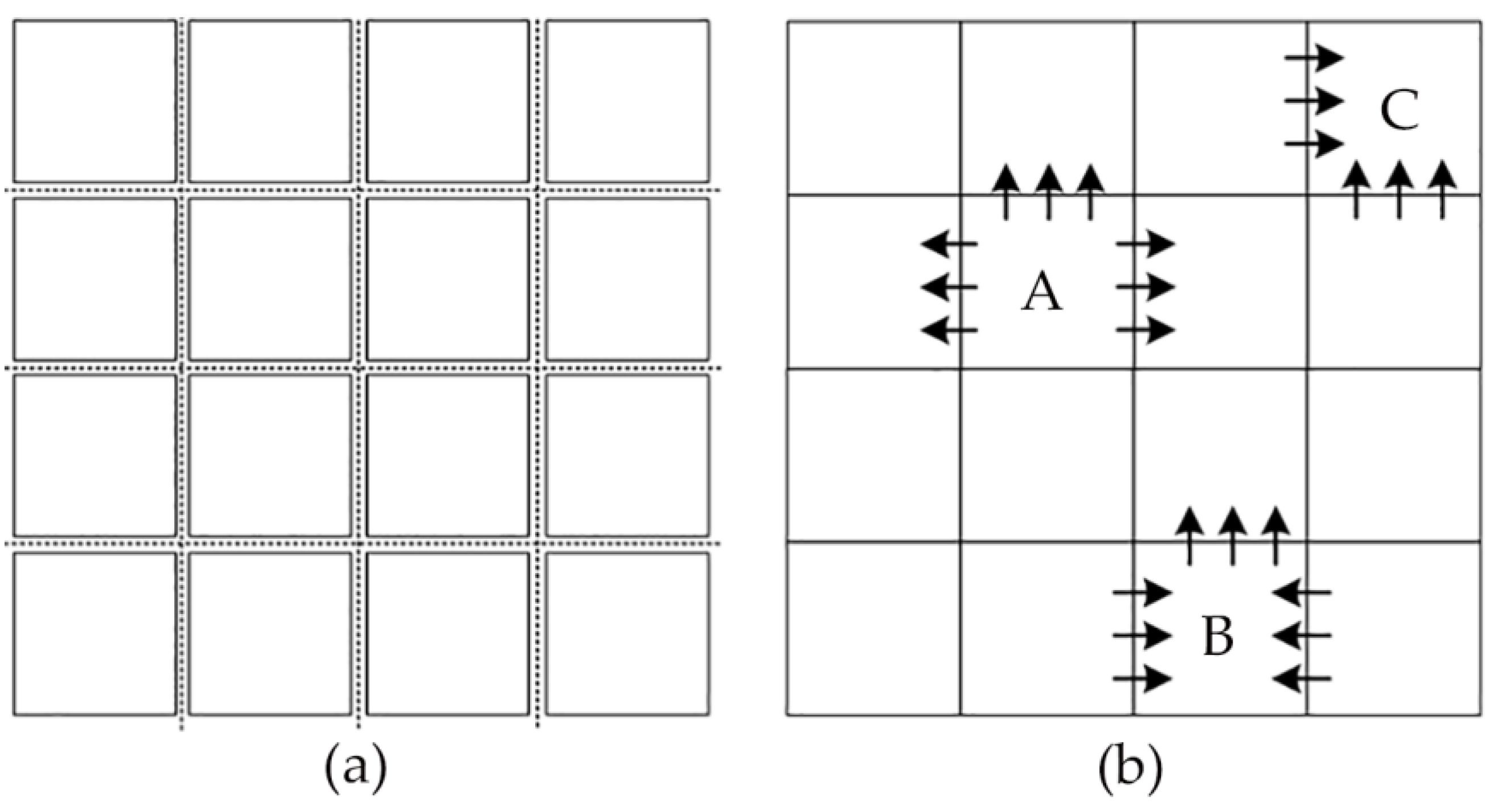
In addition, the supply-side and demand-side factors alone are not enough to explain the health workforce distribution within countries. It is important to note that the health workforce distribution within countries is different from those between countries. In Figure 1a, each square represents a country where all countries have relatively independent health labor markets because of the existence of borders and customs, and therefore, previous studies on the health workforce density differences can ignore the connections between them. When it comes to the health workforce distribution within countries (Figure 1b), each square represents one provincial unit or state, and the geographically defined health labor submarkets in provincial units or states are open and interrelated, and constant spillover effects (an economic term referring to the externalities of economic processes and activities influencing any other element not directly related to the activities where it can be both positive and negative [25]) may exist between different regions due to the frequent and massive population flow and inter-regional connections [26]. For instance, the immigration of health workforce resulting from wage gaps is the embodiment of the spillover effects between the health labor submarkets. Furthermore, overlooking spillovers also results in the inaccurate estimation of other determinants.
To summarize, the health labor market in one country should be understood as a combination of several geographically-defined health labor submarkets. It is the different dynamics in each submarket and spillovers between the submarkets that result in the unbalanced distribution of a health workforce. Figure 2 shows the “supply–demand–spillover” theoretical model built in this study to understand the dynamics and spillovers of the geographically defined health labor submarkets. Fortunately, the similarity of cultural, political, and economic settings makes it convenient to model the health labor submarkets within countries. The determinants of the health workforce size in one certain area can generally be divided into three parts: demand-side factors, supply-side factors, and spillover effects of other geographical units.
2.1.1. Demand Side
We can interpret the theoretical model from the demand side, as a population’s demand is the fundamental impetus to employ a health workforce [27]. It is important to differentiate the concepts of demand and need. The demand for health workers differs from the need for health workers, despite their correlation. The concept of demand refers to how many workers the health system wants, whereas the concept of need is normative—what it ought to be or how many health workers we should have [8]. The higher the medical needs, the more health workers are needed. While there are always some unmet medical needs that do not get reflected in the demand for health services due to multiple social and individual factors [28], the unmet needs are not so relevant to our study. For one thing, the unmet needs are more unfathomable and difficult to measure. For another, it is dubious to presume that unmet needs will lead to increasing demand and stronger motivation to recruit more health workers. In fact, the demand for health workforce is always calculated based on the demand for health services. For example, even though a large amount of people have medical needs, it will not influence the recruitment of health workforce if they do not go to the hospitals or other health institutions. Therefore, we believe that those unmet needs can be ignored when modeling the dynamics of the health labor market. That is, the demand of a health workforce is driven by the demand for health services rather than the medical needs.
2.1.2. Supply Side
Owing to a relatively underdeveloped education system and growing health services demand, we reasonably believe that the health workforce availability in China is restricted, to a large degree, by the supply side [29]. Overall, the supply of the health workforce depends on a two-stage supply chain involving education and employment [28]. We would like to interpret the supply-side factors in this process.
First, education for the health workforce is different from that of other professions because future practitioners will depend much more on the skills they receive via education; therefore, medical education is an indispensable channel to supply the workforce in health services [9]. As a result, it is appropriate to conclude that education capacity is the most prominent determinant of the supply of a health workforce.
Second, recruitment of medical graduates depends on the capacity of health institutions to attract and retain students. There are two types of employers in China’s health labor market: the public and the private sector [30]. China’s Health and Family Planning Commission is in charge of the employment of health workers in the public sector, while private sector recruitment mainly depends on the market. The attraction and retention capacity of public facilities mainly depends on government investment, since an overwhelming majority of expenditure is allocated to the health workforce [31]. Therefore, those institutions with a more opulent budget will have a greater capacity to attract health workers by offering a decent salary. In contrast, the workforce recruitment of the private sector relies predominantly on social investment. For one thing, the influx of capital into the private medical sector will enlarge employment opportunities; moreover, the competition between these two sectors may increase the working conditions of employees in both sectors, attracting more health workers on the whole.
2.1.3. Spillover Effects
Last but not least, spillover effects should not be ignored, due to the potential connections between geographical units. Therefore, the health workforce size in one provincial unit should not only be explained by the supply- and demand-side factors in the local area, but also by the interaction with other adjacent provincial units—or in the other words, the spillover effects of factors within one province on other provincial units. The stronger the supply- or demand-side factors in one area, the more likely they are to have spillover effects on the surrounding regions. For instance, if government investment in health in one unit is relatively higher than the other units, health workers from adjacent units will likely be attracted to this unit through migration flow.
2.2. Measurements
2.2.1. Health Workforce Size: Health Workforce Density
The total population of the health workforce (health workforce size) is an important indicator to evaluate health workforce availability in one region/country. However, as different regions differ in population size, the total population of the health workforce cannot be used for comparison across different regions or nations. To exclude the effect of population factors, health workforce density (the ratio of health workforce quantity to population size) is widely used as an indicator for regional comparison [4]. This study will use health workforce density as a dependent variable (DV).
As for the classification of the health workforce, China has developed its own system of nomenclature for health workers, with those health workers who deliver health services being referred to as health technicians (HTs) [32]. Health technicians in China consist of licensed doctors (LDs), registered nurses (RNs), pharmacists, technologists, and others who play various roles in health service delivery [33]. Since LDs and RNs are most closely related to the supply and coverage of health services, we will only target LDs and RNs in the discussion. To summarize, this study chose the densities of HTs, LDs, and RNs as the dependent variables; i.e., health technician density (HTD), licensed doctors density (LDD), and registered nurses density (RND).
2.2.2. Health Services Demand: Outpatient and Inpatient Health Service Utilization
By definition, health services refers to a certain quantity or a mix of different services provided by the health sector [28]. The health services in China can be divided into outpatient services and inpatient services [34]. This study adopted both the outpatient and inpatient visits, as the outpatient and inpatient services reflect different aspects of the health services. To be consistent with the DVs, we used the ratio of health services visits and the population (i.e., outpatient visits per capita, OVPA, and inpatient visits per capita, IVPA), as they can be explained as the average health services demand of the population in a certain area—more per capita inpatient and outpatient visits demonstrates a stronger health services demand.
2.2.3. Education Capacity: Number of Medical Graduates
Medical education is the cornerstone of health care, as it channels a flow of trained professionals to the health service sectors. The more medical students the education system trains, the larger the potential labor force for the health industry. Therefore, in this study, the total number of medical graduates was selected to represent education capacity in a given year. Again, to be consistent with the DVs, we used the ratio of medical graduates to the population size, or medical graduate density (MGD), as the explanatory variable for health workforce density.
2.2.4. Government and Social Investment: Government and Social Health Expenditure
In a previous study, Zaman et al. [12] used total health expenditure as an explanatory variable for health workforce density. In China, there are two statistical indicators that correspond exactly to government and social investment. Government health expenditure represents investment in medical and health services from government at all levels, while social health expenditure is the investment in medical and health services from all sectors of society, rather than the government alone [33]. We used the ratio of health expenditure to population size; that is, government health expenditure per capita (GHEPA) and social health expenditure per capita (SHEPA).
A summary of all the variables and their code, source, and expected signal are shown in Table 1.
3. Data and Methods
3.1. Data Resources
This study established a statistical model using a balanced panel data set of 31 provincial units in China, over the period 2012–2014 (only in these three years were all the data available in each provincial unit). Table S1, in the supplementary file, shows all the original data. We chose to conduct this study at a provincial level because all of the provincial units have relatively complete health labor markets as a result of the relatively independent health and education systems. Data on health workforce quantity, inpatient and outpatient services, and government and social health expenditure were obtained from the China Health and Family Planning Statistical Yearbook. Population data were obtained from the China Statistical Yearbook. Data on medical graduates were obtained from the China Education Statistical Yearbook. All data were collected at the provincial level in Mainland China, excluding Hong Kong and Macao. The maps presented in Figure 3 show the mean values of HTD, LDT, and RND from 2012 to 2014 in each provincial unit.
3.2. Spatial Panel Data Models
Analysis of the determinants and spillovers in the health labor market was based on the following model, as a result of the theoretical model and measurements provided in Section 2.
where the subscript i represents province units (i = 1, 2, …, 31); t denotes time (t = 2012, 2013, 2014). represents the constant term; and is the error term. To reduce heteroscedasticity as much as possible, all variables were in logarithmic form. This implies that the coefficient reflects the percentage change in the DVs to the independent variables (IVs), proportionately.
However, spillover effects render traditional econometric models biased and less effective. To identify factors influencing health workforce density, taking their spillovers into consideration, we employed spatial panel-data methods to examine the space–time relationship between the IVs and health workforce density. One major benefit of spatial econometric models is that they can assess the degree of spatial spillover in empirical cases [35]. They complement panel data methods by introducing econometric approaches; therefore, the statistical models are put into a space-time context, considerably increasing the accuracy of estimation.
In general, the spatial panel econometric models encompass three basic models: the spatial lag panel model (SLPM), the spatial error panel model (SEPM), and the spatial Durbin panel model (SDPM) [36,37]. The SLPM is mainly employed to analyze “the spatial autocorrelation of the DV, that is, whether the value of a geographical area is influenced by values of its neighboring regions.” [38]. The SEPM is used most often to address the spatial autocorrelation of error items [39]. The SDPM is most useful when the DV should be explained by the IVs in both the region and in other geographical units [40].
3.2.1. The Spatial Lag Panel Model
In the SLPM, Y and X, respectively, represent the vector of DVs and IVs. is a spatial weight matrix (row-standardized), built with the 31 geographical units in China. Shared borders are the criteria to build the spatial weight matrix, as explained in Equation (3). If province i is the adjacent unit of j, then = 1, while if not, then = 0. WY stands for the spatial lag (average of the neighbors) of the DV; represents the regression coefficients; stands for the spatial autocorrelation coefficient; and ε is the vector of independent disturbance terms. indicate spatial fixed effects and time-period fixed effects, respectively.
3.2.2. The Spatial Error Panel Model
The SEPM is based on the assumption that the DV is related to a group of variables, as well as the spatially autocorrelated error term. This is explained by Equation (4). represents the spatial autocorrelation coefficient, which represents the impact of the residuals of the adjacent spatial units on that target area. The rest of the parameters share the same meaning as with the SLPM.
3.2.3. The Spatial Durbin Panel Model
As shown in Equation (5), in the SDPM, are as spatial parameters, indicating the impact of the IVs in the surrounding units on the DV of the target area. The rest of the parameters share the same meanings as with the SLPM and SEPM.
3.3. Model Specification
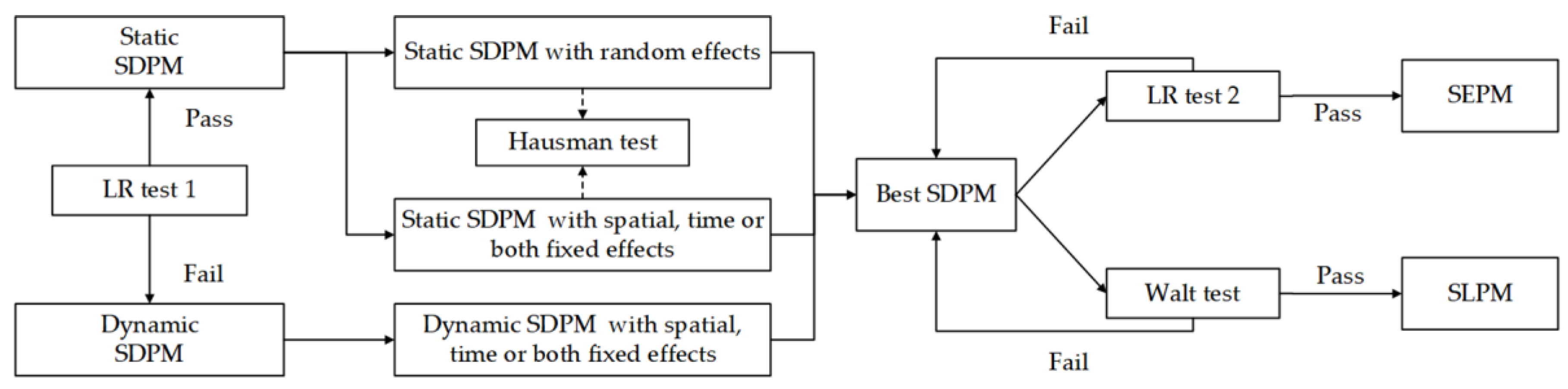
Procedures for the specification of spatial econometric panel models are shown in Figure 4. Following the strategy proposed by Elhorst [41], investigators should start with the spatial Durbin model (SDM) as a general specification and test for alternatives. We estimated the SDPM, but we also wanted to know if it was the best model for the data at hand. However, as this study dealt with the panel data, we needed to make a judgment between the static SDPM model and its dynamic form (Formula 6) in the first place with a LR (likelihood ratio) test (LR test 1: H0: δ = τ = 0). If we could not reject this null hypothesis, then the static SDPM was good enough to model the dynamics and spillovers of the health labor market. Otherwise, we should adopt its dynamic form.
After that, the model specification was divided into two steps. First, we estimated all the available SDPMs to test which one was the best. In the second step, we ran two tests to see whether the best SDPM could be simplified into the other two spatial econometric models.
In the first step, the static SDPM was divided into the model with spatial fixed effects (controlling the “space-specific, time-invariant” variables excluded from the model), the model with time fixed effects (controlling “all time-specific, space-invariant variables” excluded from the model), the model with both fixed effects (controlling the above two), and the random effects models according to different assumptions [36]. In contrast, there were only three available models for dynamic SDPM: the model with spatial fixed effects, the model with time fixed effects, and the model with both fixed effects. According to Green [43], we should select one-way fixed models (spatial fixed or time fixed) if the sample size n does not equal to T when compared with a two-way fixed model. More specifically, a model with spatial fixed effects for short panels (n > T) and mode with time fixed effects for long panels (n < T). Furthermore, the choice between the fixed effects model and random effects model should be made with the Hausman statistics [44]. In the second step, the Wald and LR test were specifically used to test the alternatives of SDPM. It was easily shown that if = 0 and ≠ 0 (Wald test: H0: = 0), the model was SLPM, while if θ = − (LR test 2: H0: θ = −), the model was SEPM, where errors are spatially correlated. However, on the condition that if the condition of θ = 0 and θ + β = 0 were both rejected, the SDPM would be the most fit model [45].
As there were too many available models for each DV, we decided to display all the dynamic and static SDPMs, as they were the starting point to do the model specification, but the results of SLPM and SEPM would be displayed when necessary.
3.4. Software
The spatial econometric panel models were computed with Stata (Version 12.0). We mainly used the XSMLE command, which is a Stata command especially designed to estimate the spatial panel data models [46].
4. Results
4.1. Descriptive Statistics
Table 2 reports the descriptive and spatial statistics for all the variables.
4.2. Empirical Results of Spatial Panel Data Models
Table 3 reports the estimation results of the determinants and spillovers of HTD. Following the procedures specified in the methods, we first did the LR test 1 (listed in the bottom of Column 2) and concluded that the dynamic SDPM was better than its static form. Then we estimated three models: dynamic SDPM with spatial fixed effects (Column 2), dynamic SDPM with time fixed effects (Column 3), dynamic SDPM with spatial and time fixed effects (Column 4). We also estimated the four static SDPM models and the Hausman test for reference. In the context of this study, the dynamic SDPM with spatial effects was preferentially compared with the time fixed and both fixed models, as the data set belonged to the short panel (n > T). Furthermore, Wald test and LR test 2 also indicated that the dynamic SDPM with spatial fixed effects could not be simplified into dynamic SEPM or dynamic SLPM.
Table 4 reports the estimation results of the determinants and spillovers of LDD. LR test 1 indicated that the static SDPM was better than its dynamic form. The Hausman test (the outcomes are listed in the bottom of Columns 5 to 8) indicated that the static SDPM with fixed effects was better than static SDPM with random effects for the estimation of determinants and spillovers for LDD. Similarly, we also adopted the static SDPM with spatial fixed effects, as the data set belonged to the short panel. To further determine whether the static SDPM model with spatial fixed effects was appropriate, we estimated the static SEPM and static SLPM with spatial fixed effects. According to the results of LR test 2 and the Wald diagnostic test, only the null hypothesis of the Wald test was rejected at the 5% significance level, indicating that the static SDPM with spatial fixed effects could be simplified into static SEPM with spatial fixed effects.
Table 5 reports the estimation results of determinants and spillovers of RND, respectively. Its models specification process was similar to that of HTD, indicating that the dynamic model with spatial fixed effects was superior to other models. Since SDPM exploits the complicated dependence structure between units, the effect of an explanatory variable change for a specific unit will affect the unit itself and potentially affect all other units indirectly. The changes of variables in the neighboring units can further affect the specific unit via feedback. Hence, the coefficients in the SPDM cannot be explained as the percentage change of DVs to the IVs, as the derivative of y with respect to x usually does not equal to βk.
Therefore, we only explain the model for LDD here. As shown in the ninth column (static SLPM with spatial fixed effects) in Table 4, the spatial autocorrelation coefficient λ was positive and significant. This implied that there was obvious spatial dependence in the labor market of licensed doctors, which meant the LDD of one province was affected by both the local unit and the neighboring provinces due to spatial spillovers. As for the independent variables, only the OVPA, IVPA, and MGD reached the 5% significance level. A 1% increase of OVPA and IVPA in one provincial unit was likely to result in 0.366% and 0.317% increase of LDD in the same provincial unit, respectively. In contrast, 1% increase of MGD yielded 0.060% increase of LDD.
4.3. Decomposition of the Direct and Spillover Effects
To better deliberate on the coefficients of the SDPM models, we further decomposed the effects of IVs on DV in SDPM models (highlighted in Table 3 and Table 5) into short-run directs and spillover (indirect) effects. By definition, the direct effects measure the influence of a unit change in IV x in provincial unit i on health workforce density in provincial unit i averaged across all the provincial units. In contrast, the spillover effects measure the influence of a unit change in variable x in all the provincial units excluding unit i on the health workforce density in provincial unit i averaged across all the provincial units. The total effects measure the impact of the same unit change in IVs in all the provincial units on health workforce density in unit i, again averaged across all provincial units; therefore, the average total effects equal the sum of average direct and average spillover effects.
A new approach was developed by LeSage and Pace [47] to measure the direct and indirect, or spatial spillover, effects in relation to changes in the exogenous variables. The SPDM (Equation (4)) is rewritten in the vector form in the following formula:
The matrix of partial derivatives of with respect to the kth exogenous variable of X in unit 1 up to unit N is represented as follows [37]:
The partial derivatives indicate “the effect of a change in a specific exogenous variable in a specific spatial location on the DV of all other locations”. The direct effect was defined by LeSage and Pace [47] as “the sum of the diagonal elements of the matrix on the right side of Equation (6), and the indirect effect as the average of either the row sums or column sums of the non-diagonal elements of the matrix”.
Table 6 shows the direct, spillover and total effects calculated based on the above-mentioned methods. First, we focused on the direct effects. The findings showed that the direct effects of OVPA, IVPA, and MGD were significant for both HTD and RND. In terms of health services demand, it was estimated that a 1% increase in OVPA in one provincial unit would lead to a 0.170% (0.119% for RND) increase in HTD in the same unit, while a 1% increase in IVPA could bring a 0.160% (0.154% for RND) increase in LDD. Surprisingly, a 1% increase in MGD could result in a 0.058% and 0.085 decrease for LDD and RND, respectively.
Regarding the spillover effects, on the demand side, the spillover effects of OVPA were negative and significant for both HTD and RND. A 1% increase in OVPA in the local provincial unit will on average lead to a 0.165% (1.205% for RND) decrease for HTD in all the neighboring units. On the supply side, the spillover effects of GHEPA and SHEPA on HTD were significant only at the 0.1 significance level. A 1% increase in GOVHE in the local unit could lead to a 0.121% (0.066% by SOCHE) increase in HTD in the neighboring units. In contrast, a 1% increase of GOVHE in the local unit could result in a 0.342% increase in RND in the neighboring units, which was significant at the 0.01 significance level. Finally, the spillover effects of MGD played a huge role in the labor market of both HT and RN. A 1% increase in MGD in the local unit could lead to 0.145% and 0.269% of HTD and RND in all the neighboring units, respectively.
5. Discussion
The distribution of the health workforce is a topic that has been intensively researched in the health field, and is relevant to the measurement of health equity—an important aspect of social fairness [48]. This study built a “supply–demand–spillover” theoretical model (Figure 2) to map the dynamics and spillovers in the health labor market, and employed spatial panel data models to empirically measure the effects of intra-regional supply-side and demand-side factors, as well as inter-regional spillover effects. The findings provide a deeper and more comprehensive understanding of the dynamics of the health labor market, as well as evidence-based health workforce allocation policies in China.
Theoretically, the contribution of this study is twofold. First, supply and demand theory in labor economics is fundamental to modeling the dynamics of the health labor market, and thus helps shape our understanding of the health workforce distribution. This study refined supply-side factors (education capacity, government investment, and social investment) and demand-side factors (health services demand) based on China’s reality; however, this theoretical model cannot explain the health workforce distribution of countries, due to the nuances and variances of health systems. Still, we believe that it provides a systematic perspective to examine the dynamics of the health labor market. Second, this study introduced spillovers into the theoretical model to help better understand the health labor market. To our knowledge, this study represents one of the first attempts to take inter-regional connections into consideration, and thus remedy the supply and demand theory deficits when applied to the health labor markets within countries. As mentioned in Section 2, the dynamics of the health labor market is closely related with the equity in health workforce distribution and also the health workforce planning. The existence of spillover effects in the health labor market indicates that the health labor submarkets in different provincial units are not independent of each other, which should be an important consideration to balance the health workforce distribution and local health workforce planning.
Empirically, the results indicated that the spillover effects of the health labor market do exist, which echoed the rationality of the theoretical model. While there exist great differences among the coefficients and significance levels of the IVs for the three different DVs, this reveals that the dynamics and spillover of the health labor market for HTs, LDs, and RNs are slightly different. We would also like to discuss the results and policy implications in accordance with the theoretical model.
From the demand side, health services demand plays an important role in health labor submarkets. First, even though demand does not solely drive health workforce size, the results confirmed the significant direct effects of health services demand on HTD, LDD, and RND, indicating that health services demand matters in the health labor market. In addition, the results indicate that the spillover effects of OVPA were significant in driving the HTD and RND. The uneven health services demand—as indicated in the results—is likely to induce brain drain of health workforce by siphoning the health talents from surrounding regions. More specifically, if there are high health services demands in one unit, it not only reveals higher health workforce density in local units, but also a likelihood of attracting the health workforce from adjacent units. Second, the results indicated that the different types of health services utilization play different roles in the health labor market. For all of the HTs and LDs, outpatient visits and inpatient visits play almost identical role in driving their densities. Regarding the RNs, the increase of inpatient visits provides more motivation to recruit RNs than outpatient visits, which can be attributed to the different roles of LDs and RNs in health service delivery, as the nurses spend most of their time in providing the inpatient services. The above-mentioned two points imply that we should proactively allocate health workforce via different kinds of health services demand. At first glance, the health services demand is objective and has nothing to do with the government. In effect, the government can also play a role in the demand side, as the medical needs of the general public are not necessarily reflected in the needs for health services proportionately. Therefore, a population’s health services demand can also be stimulated or guided through related health policies—for example, health insurance and medical aid. If we want to increase the health workforce density in one unit by appropriately guiding the health services demand of the public, the coverage of medical insurance and medical aids should be expanded to fulfill the potential medical needs (especially those repressed by economic conditions), and also prevent the potential brain drain.
From the supply side, a two-stage supply chain should be taken into consideration. First, even though the supporting role of education capacity for the intra-regional health industry is not prominent for each type of health workforce, its spillover effects are positive and significant for both HTD and RND. Therefore, it is a feasible strategy to increase the medical education capacity in remote provincial units to enhance the supply of a health workforce. However, admittedly, the supply of qualified medical students is not solely determined by the education capacity of medical institutions [8]. For one thing, as a qualified medical graduate, one needs to master the matching skills and enter the health labor market at the right time; and for another, one has a relatively long education time. Both of these conditions require the education sector to plan ahead. Second, this study failed to confirm the significant direct effects of health expenditure on health workforce density. However, the spillover effects of government and social health expenditure was both positive and significant for HTD, indicating that those remote provincial units should work together and make good use of the “visible hand” and “invisible hand”.
To conclude, supply-side factors, demand-side factors, and spillovers constitute the dynamics of the health labor market. We can easily draw lessons for health workforce policy-making in China; however, the health labor market is ultimately a complex issue. The supply-and-demand perspective aids our understanding of the health labor market. First, the health labor market is not static over time. It requires constant supply adjustments and changing guidance for supply and demand. Second, the health labor market is not monolithic across space. Although scarcity in the health workforce might be detected in one region, a nuanced picture might be drawn when zooming into smaller scales. For example, when divided into smaller patches of the submarket (e.g., urban–rural, public–private, health institution level, skill mix) [23], it is possible that health labor is sufficient in some submarkets and greatly in need in others. Third, the supply and demand sides are not mutually independent. For instance, with proper management and intervention, the health workforce allocated to disease control and prevention will reduce medical needs significantly.
This study also bears some limitations. This study only focused on the total quantity—rather than the quality—of the health workforce. It is important to note that effective health service delivery depends not only on health workforce quantity, but also on quality and skill mix [32]. Rural and remote areas experiencing a health workforce shortage usually lack a high-quality health workforce. Remote areas are confronted with three-fold health workforce challenges at the same time: the supply capacity in these areas is inadequate, they face low workforce quality, and there are draining effects from the surrounding regions. In addition, due to the lack of data in some provincial units before 2012, this study was conducted based on a three-year short panel data set, which limits the model selection. In the future, more detailed studies are suggested to zoom into smaller scales and focus on panel data spanning a longer time.
6. Conclusions
The utilization of supply and demand theory worked well when modeling the dynamics of the health labor market. Each provincial health labor market resembles the health labor market of the country, while the existence of spillover effects makes them different from independent health labor markets. No single health labor market provincial unit could get away from other units. For all policy makers, this is a clear message that equitable health workforce distribution depends on multifaceted efforts [49]. The existence of spillover effects is not only a challenge, but also an opportunity to balance and strengthen the health labor market in local areas. The role of the government lies in its coordination of multiple sectors (e.g., education, health, labor, etc.), and also in pinpointing its position in the health labor market, which depends on the foresight and profound understanding of the health labor market.
Supplementary Materials
The following are available online at https://www.mdpi.com/2071-1050/10/2/333/s1. Table S1. The original data of dependent variables and independent variables in each provincial unit during 2012–2014.
Acknowledgments
We would like to thank Xiai Shi for his helpful comments on the manuscript. We are also grateful to the referees for their helpful comments and suggestions.
Author Contributions
B.Z. and Y.F. conceived and designed the study; B.Z. collected and analyzed the data; B.Z. and Y.F. drafted the paper, J.L. and Y.M. read and revised the draft critically. All authors read and approved the final manuscript.
Conflicts of Interest
The authors declare no conflict of interest.
References
- World Health Organization. Health in 2015: From MDGs to SDGs; World Health Organization: Genova, Switherland, 2015. [Google Scholar]
- Campbell, J. The route to effective coverage is through the health worker: There are no shortcuts. Lancet 2013, 381, 725. [Google Scholar] [CrossRef]
- Doull, L.; Campbell, F. Human resources for health in fragile states. Lancet 2008, 371, 626–627. [Google Scholar] [CrossRef]
- World Health Organization. Establishing and Monitoring Benchmarks for Human Resources for Health: The Workforce Density Approach; World Health Organization: Geneva, Switzerland, 2008. [Google Scholar]
- Anand, S.; Bärnighausen, T. Human resources and health outcomes: Cross-country econometric study. Lancet 2004, 364, 1603–1609. [Google Scholar] [CrossRef]
- World Health Organization. Reassessing the Relationship between Human Resources for Health, Intervention Coverage and Health Outcomes; World Health Organization: Genova, Switherland, 2006. [Google Scholar]
- World Health Organization. World Health Statistics 2017; World Health Organization: Geneva, Switzerland, 2017. [Google Scholar]
- Dussault, G.; Vujicic, M. Demand and Supply of Human Resources for Health. Int. Encycl. Public Health 2008, 2, 77–84. [Google Scholar]
- Dussault, G.; Franceschini, M.C. Not enough there, too many here: Understanding geographical imbalances in the distribution of the health workforce. Hum. Resour. Health 2006, 4, 12. [Google Scholar] [CrossRef] [PubMed]
- Kanchanachitra, C.; Lindelow, M.; Johnston, T.; Hanvoravongchai, P.; Lorenzo, F.M.; Huong, N.L.; Wilopo, S.A.; Dela Rosa, J.F. Human resources for health in southeast Asia: Shortages, distributional challenges, and international trade in health services. Lancet 2011, 377, 769–781. [Google Scholar] [CrossRef]
- Freed, G.L.; Nahra, T.A.; Wheeler, J.R.C. Relation of per capita income and gross domestic product to the supply and distribution of pediatricians in the United States. J. Pediatr. 2004, 144, 723–728. [Google Scholar] [CrossRef] [PubMed]
- Zaman, R.U.; Gemmell, I.; Lievens, T. Factors Affecting Health Worker Density: Evidence from a Quantitative Cross-Country Analysis. SSRN Electron. J. 2014, 1–17. [Google Scholar] [CrossRef]
- Chen, L.C. Striking the right balance: Health workforce retention in remote and rural areas. Bull. World Health Organ. 2010, 88. [Google Scholar] [CrossRef] [PubMed]
- Bonenberger, M.; Aikins, M.; Akweongo, P.; Wyss, K. The effects of health worker motivation and job satisfaction on turnover intention in Ghana: A cross-sectional study. Hum. Resour. Health 2014, 12, 43. [Google Scholar] [CrossRef] [PubMed] [Green Version]
- Fogarty, L.; Kim, Y.M.; Juon, H.; Tappis, H.; Noh, J.W.; Zainullah, P. Job satisfaction and retention of health-care providers in Afghanistan and Malawi. Hum. Resour. Health 2014, 12, 11. [Google Scholar] [CrossRef] [PubMed]
- Zhang, Y.; Feng, X. The relationship between job satisfaction, burnout, and turnover intention among physicians from urban state-owned medical institutions in Hubei, China: A cross-sectional study. BMC Health Serv. Res. 2011, 11, 235. [Google Scholar] [CrossRef] [PubMed] [Green Version]
- Scholz, S.; Schulenburg, J.-M.; Greiner, W. Regional differences of outpatient physician supply as a theoretical economic and empirical generalized linear model. Hum. Resour. Health 2015, 13, 85. [Google Scholar] [CrossRef] [PubMed]
- Waters, H.R. Measuring equity in access to health care. Soc. Sci. Med. 2000, 51, 599–612. [Google Scholar] [CrossRef]
- WHO Closing the gap in a generation: Health equity through action on the social determinants of health. Lancet 2008, 372, 1661–1669. [CrossRef]
- Shadmi, E.; Wong, W.C.W.; Kinder, K.; Heath, I.; Kidd, M. Primary Care Priorities in Addressing Health Equity: Summary of the WONCA 2013 Health Equity Workshop. Int. J. Equity Health 2014, 13, 104. [Google Scholar] [CrossRef] [PubMed]
- Culyer, A.J.; Wagstaff, A. Equity and equality in health and health care. J. Health Econ. 1993, 12, 431–457. [Google Scholar] [CrossRef]
- Liu, J.X.; Goryakin, Y.; Maeda, A.; Bruckner, T.; Scheffler, R. Global Health Workforce Labor Market Projections for 2030. Hum. Resour. Health 2017, 15, 1–12. [Google Scholar] [CrossRef] [PubMed]
- McPake, B.; Scott, A.; Edoka, I.; McPake, B.; Scott, A. Analyzing Markets for Health Workers: Insights from Labor and Health Economics; World Bank: Washington, DC, USA, 2014; ISBN 978-1-4648-0224-9. [Google Scholar]
- McRae, I.; Butler, J.R.G. Supply and demand in physician markets: A panel data analysis of GP services in Australia. Int. J. Health Care Financ. Econ. 2014, 14, 269–287. [Google Scholar] [CrossRef] [PubMed]
- Yang, Y.; Wong, K.K.F. A Spatial Econometric Approach to Model Spillover Effects in Tourism Flows. J. Travel Res. 2012, 51, 768–778. [Google Scholar] [CrossRef]
- Fu, Y.; Gabriel, S.A. Labor migration, human capital agglomeration and regional development in China. Reg. Sci. Urban Econ. 2012, 42, 473–484. [Google Scholar] [CrossRef]
- Murphy, T.G.; MacKenzie, A.; Guy-Walker, J.; Walker, C. Needs-based human resources for health planning in Jamaica: Using simulation modelling to inform policy options for pharmacists in the public sector. Hum. Resour. Health 2014, 12, 67. [Google Scholar] [CrossRef] [PubMed]
- Vujicic, M.; Zurn, P. The dynamics of the health labour market. Int. J. Health Plan. Manag. 2006, 21, 101–115. [Google Scholar] [CrossRef]
- Zhu, J.; Li, W.; Chen, L. Doctors in China: Improving quality through modernisation of residency education. Lancet 2016, 388, 1922–1929. [Google Scholar] [CrossRef]
- Xu, J.; Liu, G.; Deng, G.; Li, L.; Xiong, X.; Basu, K. A comparison of outpatient healthcare expenditures between public and private medical institutions in urban China: An instrumental variable approach. Health Econ. 2015, 24, 270–279. [Google Scholar] [CrossRef] [PubMed]
- Ranson, M.K.; Chopra, M.; Atkins, S.; Dal Poz, M.R.; Bennett, S. Priorities for research into human resources for health in low- and middle-income countries. Bull. World Health Organ. 2010, 88, 435–443. [Google Scholar] [CrossRef] [PubMed]
- Anand, S.; Fan, V.Y.; Zhang, J.; Zhang, L.; Ke, Y.; Dong, Z.; Chen, L.C. China’s human resources for health: Quantity, quality, and distribution. Lancet 2008, 372, 1774–1781. [Google Scholar] [CrossRef]
- National Health and Family Planning Commission of the PRC. China Health and Family Planning Statistical Yearbook 2016; Chinese Peking Union Medical College Press: Beijing, China, 2016.
- Lv, Y.; Xue, C.; Ge, Y.; Ye, F.; Liu, X.; Liu, Y.; Zhang, L. Analysis of factors influencing inpatient and outpatient satisfaction with the Chinese military health service. PLoS ONE. 2016, 11, e0151234. [Google Scholar] [CrossRef] [PubMed]
- Liu, Y.; Xiao, H.; Zikhali, P.; Lv, Y. Carbon Emissions in China: A Spatial Econometric Analysis at the Regional Level. Sustainability 2014, 6, 6005–6023. [Google Scholar] [CrossRef]
- Jiang, L.; Ji, M. China’s Energy Intensity, Determinants and Spatial Effects. Sustainability 2016, 8, 544. [Google Scholar] [CrossRef]
- Zhou, Z.; Ye, X.; Ge, X. The Impacts of Technical Progress on Sulfur Dioxide Kuznets Curve in China: A Spatial Panel Data Approach. Sustainability 2017, 9, 674. [Google Scholar] [CrossRef]
- Cheng, Y.; Wang, Z.; Ye, X.; Wei, Y.D. Spatiotemporal dynamics of carbon intensity from energy consumption in China. J. Geogr. Sci. 2014, 24, 631–650. [Google Scholar] [CrossRef]
- Long, R.; Shao, T.; Chen, H. Spatial econometric analysis of China’s province-level industrial carbon productivity and its influencing factors. Appl. Energy 2016, 166, 210–219. [Google Scholar] [CrossRef]
- Huang, J.; Xia, J. Regional competition, heterogeneous factors and pollution intensity in China: A spatial econometric analysis. Sustainability 2016, 8, 171. [Google Scholar] [CrossRef]
- Elhorst, P.; Piras, G.; Arbia, G. Growth and Convergence in a Multiregional Model with Space-Time Dynamics. Geogr. Anal. 2010, 42, 338–355. [Google Scholar] [CrossRef]
- Elhorst, J.P. Applied Spatial Econometrics: Raising the Bar. Spat. Econ. Anal. 2010, 5, 9–28. [Google Scholar] [CrossRef]
- Greene, W.H. Econometric Analysis, 7th ed.; Prentice Hall: Upper Saddle River, NJ, USA, 2012; ISBN 9780131395381. [Google Scholar]
- Hausman, J. Specification tests in econemetrics. Work. Pap. 1976, 46, 1251–1271. [Google Scholar]
- Kang, Y.Q.; Zhao, T.; Wu, P. Impacts of energy-related CO2 emissions in China: A spatial panel data technique. Nat. Hazards 2016, 81, 405–421. [Google Scholar] [CrossRef]
- Hughes, G. XSMLE: Stata module for spatial panel data models estimation. Stata J. 2017, 17, 139–180. [Google Scholar]
- Lesage, J.; Pace, R.K. Introduction to Spatial Econometrics; CRC Press: Boca Raton, FL, USA, 2009; ISBN 2008038890. [Google Scholar]
- Liu, W.; Liu, Y.; Twum, P.; Li, S. National equity of health resource allocation in China: Data from 2009 to 2013. Int. J. Equity Health 2016, 15, 68. [Google Scholar] [CrossRef] [PubMed]
- World Health Organization. A Universal Truth: No Health Without a Workforce; World Health Organization: Genova, Switherland, 2013. [Google Scholar]
Figure 1.
(a) Mutually-independent health labor markets between countries and (b) interrelated health labor submarkets within countries.
Figure 1.
(a) Mutually-independent health labor markets between countries and (b) interrelated health labor submarkets within countries.

Figure 2.
Supply–demand–spillover model.
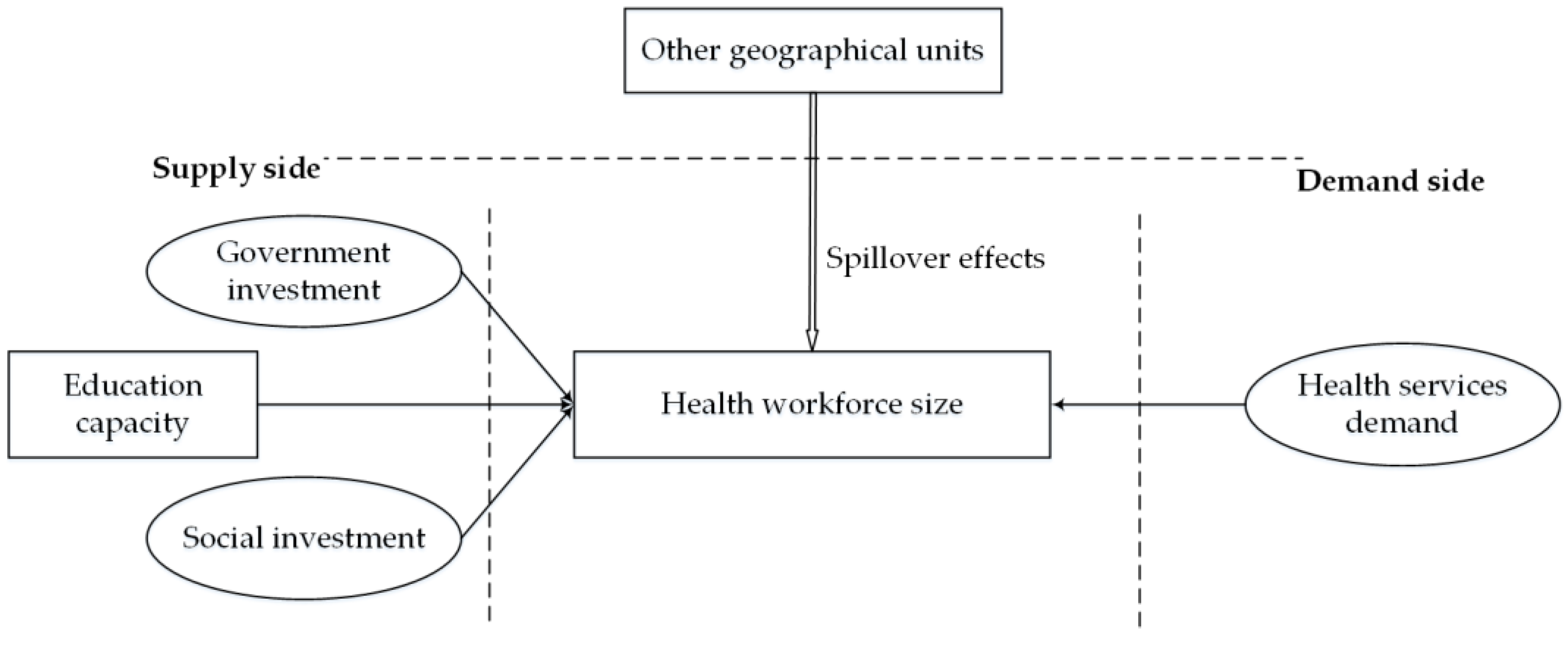
Figure 3.
The average density of three categories of the health workforce at the provincial level (2012–2014).
Figure 3.
The average density of three categories of the health workforce at the provincial level (2012–2014).
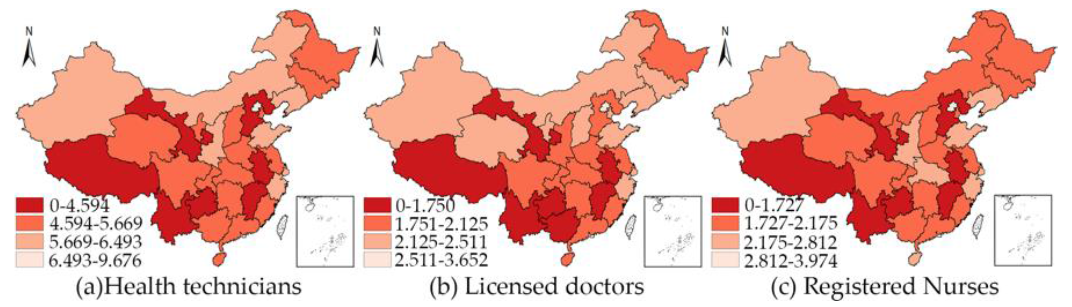
Figure 4.
Model specification procedures of the spatial econometric panel models [42]. LR: likelihood ratio; SDPM: spatial Durbin panel model; SEPM: spatial error panel model; SLPM: spatial lag panel model.
Figure 4.
Model specification procedures of the spatial econometric panel models [42]. LR: likelihood ratio; SDPM: spatial Durbin panel model; SEPM: spatial error panel model; SLPM: spatial lag panel model.

Table 1.
Definition of variables, code, source, and expected signal.
| Variable Name | Measurement | Code | Description | Expected Signal |
|---|---|---|---|---|
| Health workforce density | Health technician density | HTD | Number of health technicians divided by the population and multiplied by 1000 | Dependent variable |
| Licensed doctor density | LDD | Number of licensed doctors divided by the population and multiplied by 1000 | Dependent variable | |
| Registered nurse density | RND | Number of registered nurses divided by the population and multiplied by 1000 | Dependent variable | |
| Health services demand | Outpatient visits per capita | OVPA | Number of outpatient visits divided by the population | + |
| Inpatient visits per capita | IVPA | Number of inpatient visits divided by the population | + | |
| Government investment | Government health expenditure per capita | GHEPA | Government health expenditure divided by the population | + |
| Social Investment | Social health expenditure per capita | SHEPA | Social health expenditure divided by the population | + |
| Education capacity | Medical graduate density | MGD | Number of medical graduates divided by the population and multiplied by 1000 | + |
Table 2.
Descriptive and spatial statistics of the variables 1.
| Variables | Obs | Mean | Std err | Minimum | Maximum | Unit | Moran’s I (2012/2013/2014) | ||
|---|---|---|---|---|---|---|---|---|---|
| HTD | 93 | 5.376 | 1.098 | 3.031 | 9.909 | Person/1000 population | 0.061 | −0.029 | −0.056 |
| LDD | 93 | 2.073 | 0.413 | 1.312 | 3.715 | Person/1000 population | 0.195 ** | 0.127 | 0.127 |
| RND | 93 | 2.056 | 0.531 | 0.562 | 4.112 | Person/1000 population | −0.008 | −0.075 | −0.099 |
| OVPA | 93 | 5.184 | 1.713 | 3.007 | 10.330 | Times/person | 0.369 *** | 0.389 *** | 0.415 *** |
| IVPA | 93 | 0.136 | 0.030 | 0.047 | 0.213 | Times/person | 0.004 | 0.136 | 0.132 |
| GHEPA | 93 | 8.018 | 2.854 | 4.982 | 18.326 | Yuan/person | 0.161 * | 0.177 * | 0.193 ** |
| SHEPA | 93 | 9.560 | 6.827 | 2.812 | 4.138 | Yuan/person | 0.234 *** | 0.215 ** | 0.238 *** |
| MGD | 93 | 0.249 | 0.093 | 0.056 | 0.489 | Person/1000 population | 0.107 | 0.120 | 0.142 |
1 * Statistical significance at 10% level; ** Statistical significance at 5% level; *** Statistical significance at 1% level.
Table 3.
Estimation of the spatial panel data models for health technician density.
| Variables | Dynamic SDPM with Spatial Fixed Effects (Best Model) | Dynamic SDPM with Time Fixed Effects | Dynamic SDPM with Spatial and Time Fixed Effects | Static SDPM with Spatial Fixed Effects | Static SDPM with Time Fixed Effects | Static SDPM with Spatial and Time Fixed Effects | Static SDPM with Random Effects |
|---|---|---|---|---|---|---|---|
| Ln(HTD)t-1 | 0.273 *** (0.051) | 1.365 *** (0.035) | 0.261 *** (0.053) | ||||
| Ln(OVPA) | 0.162 ** (0.080) | −0.044 *** (0.017) | 0.174 ** (0.083) | 0.260 *** (0.099) | 0.066 (0.051) | 0.246 ** (0.101) | 0.224 *** (0.077) |
| Ln(IVPA) | 0.163 *** (0.058) | −0.157 *** (0.020) | 0.151 ** (0.062) | 0.244 *** (0.058) | 0.187 *** (0.050) | 0.288 *** (0.065) | 0.257 *** (0.055) |
| Ln(GHEPA) | −0.034 (0.051) | −0.084 *** (0.016) | −0.051 (0.063) | 0.059 (0.068) | 0.167 *** (0.045) | 0.103 (0.077) | 0.218 *** (0.061) |
| Ln(SHEPA) | 0.009 (0.018) | −0.096 *** (0.013) | 0.006 (0.019) | 0.051 * (0.028) | 0.233 *** (0.030) | 0.066 ** (0.030) | 0.125 *** (0.035) |
| Ln(MGD) | −0.057 *** (0.019) | 0.012 (0.010) | −0.054 *** (0.019) | 0.097 *** (0.023) | 0.017 (0.029) | 0.088 *** (0.024) | 0.079 *** (0.027) |
| W*Ln(HTD)t-1 | 0.148 (0.112) | −0.708 *** (0.179) | 0.155 (0.112) | ||||
| W*Ln(OVPA) | −0.603 *** (0.171) | −0.093 *** (0.029) | −0.605 *** (0.170) | 0.456 * (0.198) | −0.120 (0.081) | −0.425 * (0.244) | −0.207 * (0.125) |
| W*Ln(IVPA) | 0.001 (0.113) | 0.487 *** (0.042) | −0.068 (0.184) | −0.194 * (0.117) | −0.605 *** (0.934) | −0.073 (0.141) | −0.316 *** (0.097) |
| W*Ln(GHEPA) | 0.126 * (0.066) | 0.172 *** (0.032) | 0.103 (0.080) | 0.040 (0.099) | −0.281 *** (0.090) | 0.137 (0.126) | −0.089 (0.089) |
| W*Ln(SHEPA) | 0.067 * (0.036) | 0.349 *** (0.033) | 0.065 * (0.036) | −0.013 (0.056) | −0.165 ** (0.082) | 0.033 (0.063) | −0.093 (0.063) |
| W*Ln(MGD) | 0.145 *** (0.039) | −0.021 (0.020) | 0.136 *** (0.053) | −0.020 (0.044) | 0.086 (0.057) | −0.031 (0.053) | 0.039 (0.053) |
| 0.047 (0.821) | 0.134 (0.195) | 0.045 (0.205) | 0.691 *** (0.092) | 0.178 *** (0.137) | 0.640 *** (0.106) | 0.566 *** (0.106) | |
| Log-likelihood | 227.3960 | 104.5904 | 213.8366 | 255.3358 | 106.3628 | 256.3851 | 161.6481 |
| Rw2 | 0.9451 | 0.7554 | 0.9373 | 0.8785 | 0.0077 | 0.8546 | 0.8583 |
| Rb2 | 0.3564 | 0.9464 | 0.3624 | 0.2589 | 0.8421 | 0.2426 | 0.7004 |
| R2 | 0.3689 | 0.9208 | 0.3734 | 0.3104 | 0.6831 | 0.2699 | 0.7139 |
| Obs | 62 | 62 | 62 | 93 | 93 | 93 | 93 |
| Test | LR test 1 H0: | LR test 2 H0: | Wald test H0: | Hausman test H0: difference in coeffs. not systematic (random effects is preferred) | |||
| 29.57 p = 0.0000 | 34.53 p = 0.0000 | 27.64 p = 0.0000 | p = 0.1151 | ||||
Note: Standard errors are in parentheses. * Statistical significance at 10% level; ** Statistical significance at 5% level; *** Statistical significance at 1% level.
Table 4.
Estimation of the spatial panel data models for licensed doctor density.
| Variables | Dynamic SDPM with Spatial Fixed Effects | Dynamic SDPM with Time Fixed Effects | Dynamic SDPM with Spatial and Time Fixed Effects | Static SDPM with Spatial Fixed Effects | Static SDPM with Time Fixed Effects | Static SDPM with Spatial and Time Fixed Effects | Static SDPM with Random Effects | Static SEPM with Spatial Fixed Effects (Best Model) | Static SLPM with Spatial Fixed Effects |
|---|---|---|---|---|---|---|---|---|---|
| Ln(LDD)t-1 | 0.139 ** (0.064) | 1.257 *** (0.042) | 0.169 *** (0.064) | ||||||
| Ln(OVPA) | 0.423 *** (0.114) | −0.028 (0.023) | 0.342 *** (0.115) | 0.420 *** (0.106) | 0.006 (0.053) | 0.420 *** (0.104) | 0.286 *** (0.080) | 0.366 *** (0.104) | 0.350 *** (0.111) |
| Ln(IVPA) | 0.069 (0.086) | −0.078 *** (0.024) | 0.131 (0.088) | 0.282 *** (0.062) | 0.048 (0.052) | 0.363 *** (0.065) | 0.231 *** (0.059) | 0.317 *** (0.060) | 0.282 *** (0.067) |
| Ln(GHEPA) | −0.076 (0.070) | −0.027 (0.019) | 0.057 (0.088) | 0.097 (0.073) | 0.080 * (0.046) | 0.207 *** (0.080) | 0.199 *** (0.060) | −0.002 (0.050) | −0.043 (0.057) |
| Ln(SHEPA) | 0.025 (0.027) | −0.059 *** (0.016) | 0.046 * (0.028) | 0.052 * (0.030) | 0.216 *** (0.032) | 0.089 *** (0.032) | 0.089 *** (0.033) | 0.039 (0.028) | 0.027 (0.029) |
| Ln(MGD) | −0.046 * (0.026) | 0.002 (0.014) | −0.052 ** (0.025) | 0.072 *** (0.026) | 0.004 (0.031) | 0.060 ** (0.025) | 0.059 ** (0.028) | 0.060 *** (0.026) | 0.073 *** (0.028) |
| W*Ln(LDD)t-1 | −0.036 (0.118) | −0.362 ** (0.176) | −0.030 (0.114) | ||||||
| W*Ln(OVPA) | −0.286 (0.270) | 0.013 (0.039) | −0.236 (0.263) | −0.311 (0.223) | −0.297 *** (0.085) | −0.021 (0.227) | −0.316 ** (0.128) | ||
| W*Ln(IVPA) | −0.061 (0.157) | 0.280 *** (0.048) | 0.414 (0.255) | −0.334 *** (0.121) | −0.582 *** (0.094) | −0.066 (0.147) | −0.406 *** (0.095) | ||
| W*Ln(GHEPA) | 0.077 (0.097) | 0.061 (0.039) | 0.227 ** (0.114) | 0.012 (0.107) | −0.020 (0.094) | 0.245 * (0.130) | −0.033 (0.091) | ||
| W*Ln(SHEPA) | 0.113 ** (0.054) | 0.139 *** (0.042) | 0.143 *** (0.053) | −0.034 (0.061) | 0.059 (0.087) | 0.054 (0.067) | −0.040 (0.064) | ||
| W*Ln(MGD) | 0.178 *** (0.057) | −0.032 (0.027) | 0.234 *** (0.060) | 0.031 (0.048) | 0.259 *** (0.060) | 0.037 (0.056) | 0.096 * (0.055) | ||
| 0.264 (0.208) | 0.015 (0.186) | 0.305 * (0.207) | 0.476 *** (0.116) | −0.108 (0.144) | 0.276 * (0.142) | 0.451 *** (0.110) | 0.165 (0.101) | ||
| λ | 0.451 *** (0.122) | ||||||||
| Log-likelihood | 202.4587 | 111.1660 | −137.0610 | 213.9414 | 213.9414 | 213.9414 | 213.9414 | 213.9414 | 148.4190 |
| Rw2 | 0.7514 | 0.4862 | 0.7060 | 0.8453 | 0.4271 | 0.7786 | 0.8186 | 0.8397 | 0.8368 |
| Rb2 | 0.4819 | 0.9712 | 0.3824 | 0.4237 | 0.8352 | 0.3119 | 0.6556 | 0.1591 | 0.4212 |
| R2 | 0.4847 | 0.9323 | 0.3813 | 0.4461 | 0.8103 | 0.3283 | 0.6654 | 0.1892 | 0.4395 |
| Obs | 62 | 62 | 62 | 93 | 93 | 93 | 93 | 93 | 93 |
| Test | LR test 1 H0: | Hausman test H0: difference in coeffs. not systematic (random effects is preferred) | LR test 2 H0: | Wald test H0: | |||||
| 0.96 p = 0.6195 | p = 0.0988 | p = 0.1835 | p = 0.0254 | ||||||
Note: Standard errors are in parentheses. * Statistical significance at 10% level; ** Statistical significance at 5% level; *** Statistical significance at 1% level.
Table 5.
Estimation of the spatial panel data models for registered nurse density.
| Variables | Dynamic SDPM with Spatial Fixed Effects (Best Model) | Dynamic SDPM with Time Fixed Effects | Dynamic SDPM with Spatial and Time Fixed Effects | Static SDPM with Spatial Fixed Effects | Static SDPM with Time Fixed Effects | Static SDPM with Spatial and Time Fixed Effects | Static SDPM with Random Effects |
|---|---|---|---|---|---|---|---|
| Ln(RND)t-1 | 0.251 ** (0.061) | 1.108 *** (0.033) | 0.206 *** (0.062) | ||||
| Ln(OVPA) | 0.146 * (0.134) | 0.013 (0.023) | 0.188 (0.131) | 0.142 (0.151) | 0.067 (0.068) | 0.141 (0.154) | 0.152 (0.108) |
| Ln(IVPA) | 0.156 (0.093) | −0.152 *** (0.032) | 0.105 (0.095) | 0.395 *** (0.090) | 0.054 *** (0.068) | 0.417 *** (0.097) | 0.512 *** (0.088) |
| Ln(GHEPA) | −0.067 (0.090) | −0.065 *** (0.023) | −0.148 (0.102) | 0.069 (0.103) | 0.146 ** (0.063) | 0.099 (0.116) | 0.206 ** (0.086) |
| Ln(SHEPA) | −0.014 (0.030) | 0.055 *** (0.016) | −0.032 (0.030) | 0.022 (0.043) | 0.292 *** (0.412) | 0.032 (0.046) | 0.169 *** (0.054) |
| Ln(MGD) | −0.093 *** (0.030) | −0.012 (0.014) | −0.080 *** (0.030) | 0.141 *** (0.036) | 0.044 (0.040) | 0.137 *** (0.037) | 0.130 *** (0.041) |
| W*Ln(RND)t-1 | 0.148 (0.140) | −0.401 ** (0.185) | 0.180 (0.137) | ||||
| W*Ln(OVPA) | −1.054 *** (0.278) | −0.096 *** (0.036) | −1.092 *** (0.266) | −0.487 (0.301) | 0.140 (0.106) | −0.427 (0.370) | 0.048 (0.179) |
| W*Ln(IVPA) | 0.054 (0.192) | 0.479 *** (0.068) | −0.292 (0.281) | −0.178 (0.191) | −1.004 *** (0.142) | −0.119 (0.213) | −0.464 *** (0.155) |
| W*Ln(GHEPA) | 0.316 *** (0.110) | 0.045 (0.047) | 0.190 (0.129) | 0.118 (0.153) | −0.633 *** (0.124) | 0.177 (0.184) | −0.100 (0.130) |
| W*Ln(SHEPA) | 0.082 (0.060) | 0.229 *** (0.046) | 0.075 (0.057) | 0.040 (0.085) | −0.262 ** (0.112) | 0.060 (0.097) | −0.080 (0.095) |
| W*Ln(MGD) | 0.246 *** (0.624) | 0.023 (0.026) | 0.200 *** (0.065) | 0.025 (0.069) | 0.008 (0.077) | 0.029 (0.083) | 0.086 (0.079) |
| 0.264 (0.208) | 0.053 (0.205) | 0.063 (0.061) | 0.499 *** (0.127) | 0.217 (0.148) | 0.481 *** (0.131) | 0.372 *** (0.129) | |
| Log-likelihood | 197.6481 | 122.6483 | 12.2820 | 202.4587 | 202.4587 | 202.4587 | 202.4587 |
| Rw2 | 0.9402 | 0.7551 | 0.5599 | 0.9030 | 0.6504 | 0.8982 | 0.8797 |
| Rb2 | 0.0330 | 0.9880 | 0.0434 | 0.0751 | 0.8706 | 0.1178 | 0.7327 |
| R2 | 0.0428 | 0.9734 | 0.0457 | 0.1294 | 0.6087 | 0.1825 | 0.7439 |
| Obs | 62 | 62 | 62 | 93 | 93 | 93 | 93 |
| Test | LR test 1 H0: | LR test H0: | Wald test H0: | Hausman test H0: difference in coeffs not systematic (random effects is preferred) | |||
| 17.97 p = 0.0001 | p = 0.0000 | p = 0.0000 | p = 0.0975 | ||||
Note: Standard errors are in parentheses. * Statistical significance at 10% level; ** Statistical significance at 5% level; *** Statistical significance at 1% level.
Table 6.
Direct, spillover, and total effects.
| Variables | Direct Effects | Spillover Effects | Total Effects | |
|---|---|---|---|---|
| Health Technicians | Ln(OVPA) | 0.170 *** (0.077) | −0.615 *** (0.204) | −0.445 ** (0.222) |
| Ln(IVPA) | 0.160 *** (0.060) | −0.002 (0.115) | 0.158 (0.114) | |
| Ln(GHEPA) | −0.033 (0.048) | 0.121 * (0.066) | 0.088 (0.061) | |
| Ln(SHEPA) | 0.007 (0.019) | 0.066 * (0.035) | 0.074 ** (0.034) | |
| Ln(MGD) | −0.058 *** (0.018) | 0.145 *** (0.040) | 0.088 ** (0.037) | |
| Registered Nurses | Ln(OVPA) | 0.119 *** (0.124) | −1.205 *** (0.414) | −1.086 ** (0.454) |
| Ln(IVPA) | 0.154 *** (0.095) | 0.086 (0.227) | 0.240 (0.241) | |
| Ln(GHPAE) | −0.054 (0.080) | 0.342 *** (0.129) | 0.288 ** (0.118) | |
| Ln(SHEPA) | −0.013 (0.030) | 0.093 (0.068) | 0.080 (0.068) | |
| Ln(MGD) | −0.085 *** (0.028) | 0.269 *** (0.078) | 0.184 ** (0.078) |
© 2018 by the authors. Licensee MDPI, Basel, Switzerland. This article is an open access article distributed under the terms and conditions of the Creative Commons Attribution (CC BY) license (http://creativecommons.org/licenses/by/4.0/).
Share and Cite
MDPI and ACS Style
Zhu, B.; Fu, Y.; Liu, J.; Mao, Y. Modeling the Dynamics and Spillovers of the Health Labor Market: Evidence from China’s Provincial Panel Data. Sustainability 2018, 10, 333. https://doi.org/10.3390/su10020333
AMA Style
Zhu B, Fu Y, Liu J, Mao Y. Modeling the Dynamics and Spillovers of the Health Labor Market: Evidence from China’s Provincial Panel Data. Sustainability. 2018; 10(2):333. https://doi.org/10.3390/su10020333
Chicago/Turabian StyleZhu, Bin, Yang Fu, Jinlin Liu, and Ying Mao. 2018. "Modeling the Dynamics and Spillovers of the Health Labor Market: Evidence from China’s Provincial Panel Data" Sustainability 10, no. 2: 333. https://doi.org/10.3390/su10020333
Note that from the first issue of 2016, this journal uses article numbers instead of page numbers. See further details here.