To License or Not to License Remanufacturing Business?


1
School of Management, Yangtze University, Jinzhou 434023, China
2
School of Economics and Management, Southwest Jiaotong University, Chengdu 610031, China
*
Authors to whom correspondence should be addressed.
Sustainability 2018, 10(2), 347; https://doi.org/10.3390/su10020347
Submission received: 4 December 2017
/
Revised: 16 January 2018
/
Accepted: 25 January 2018
/
Published: 29 January 2018
(This article belongs to the Special Issue Resilient, Sustainable and Smart Cities: Emerging Trends and Approaches)
Abstract
:Many original equipment manufacturers (OEMs) face the choice of whether to license an independent remanufacturer (IR) to remanufacture their used products. In this paper, we develop closed-loop supply chain models with licensed and unlicensed remanufacturing operations to analyze the competition and cooperation between an OEM and an IR. The OEM sells new products and collects used products through trade-ins, while the IR intercepts the OEM’s cores to produce remanufactured products and sell them in the same market. We derive optimal decisions for each of the two types of firms in licensed and unlicensed remanufacturing scenarios and identify conditions under which the OEM and the IR would be most likely to cooperate with each other in implementing remanufacturing. The results show although it is beneficial for an OEM to license an IR to remanufacture its cores, it is not always necessary for an IR to accept OEM’s authorization. Moreover, we contrast the result for licensed remanufacturing scenario in the decentralized system with that in the centrally coordinated system to quantify potential inefficiency resulting from decentralization of decision making.
1. Introduction
As one of the important means of product recovery [1], remanufacturing is a process in which old products are disassembled and their parts are repaired and used in the production of remanufactured products [2]. Examples of remanufactured products include automotive parts, computers, furniture, carpets, power tools, telephones, televisions and refrigerators, etc. Successful industry leaders, such as Kodak [3], BMW, IBM, DEC and Xerox [4], demonstrate that remanufacturing is profitable and environmentally friendly. Consequently, original equipment manufacturers (OEMs) are increasingly encouraged to invest in remanufacturing. However, not all OEMs have the infrastructure and expertise to remanufacture used products in a profitable manner [5]. By surveying thousands of remanufacturing companies, Hauser and Lund [6] found that only 6% of those companies are OEMs.
Cooperating with independent remanufacturers (IRs) in remanufacturing can be an ideal option for OEMs. For example, Cat Reman remanufactures for customers spanning several industries such as Perkins and Alcoa, Ford, and Honeywell [7]. As the largest automobile gearbox remanufacturer in China, Xin Meifu is authorized by the world’s two largest gearbox manufacturers, i.e., ZF Friedrichshafen AG and Aisin [8]. OEMs focus mainly on new product development and manufacturing and generally do not invest in remanufacturing capability. Cooperating with IRs in remanufacturing allows OEMs to keep their positive market reputation, given the fact that many IRs collect and remanufacture used products without OEMs’ authorization. For example, HP works with closely vetted reuse and recycling vendors to ensure environmentally responsible and high value recovery options. Lenovo also has an audit program to inspect recycling partners to ensure the quality of remanufactured products [9]. For IRs, accepting OEM’s authorization can increase consumers’ acceptance of remanufactured products, increase the sales of remanufactured products, and increase the cost saving from remanufacturing.
There seems to be a “win-win” solution when OEMs and IRs cooperate with each other. However, on the OEM’s side, the existence of remanufactured products may erode the market share of new products and cause cannibalization problems; on the IR’s side, a royalty fee has to be paid if it accepts the OEM’s authorization. Therefore, OEMs have to weigh pros and cons of licensing or not licensing remanufacturing business. And IRs will also decide whether to cooperate with OEMs. These considerations motivate us to examine the following questions:
- (1)
- Is it optimal for OEMs to license remanufacturing? And is it optimal for IRs to accept the licensing? Under what conditions will they cooperate with each other?
- (2)
- What are the optimal decisions of OEMs and IRs when they cooperate with each other or choose not to?
Additionally, in view of the simultaneous role of cooperation and competition between OEMs and IRs in licensed remanufacturing, it is intriguing to speculate whether central coordination could contribute to achieve a “win-win” result. What will be the difference in their optimal decisions in the decentralized and centralized decision-making systems?
In this paper, we will examine the above questions by considering three settings: (a) when OEMs choose to not license remanufacturing, OEMs and IRs operate independently; (b) when OEMs choose to license remanufacturing, IRs carry out remanufacturing with OEM’s permission and pay OEMs a royalty fee; and (c) in a centrally coordinated system, OEMs and IRs jointly make their decisions to maximize their total profits.
The rest of this paper is organized as follows. In the following section, we briefly review previous research. Section 3 presents the description and construction of our models. Section 4 details the optimal strategies of OEMs and IRs in licensed remanufacturing and unlicensed remanufacturing scenarios. Section 5 concludes the paper. All proofs are provided in Appendix A.
2. Literature Review
This paper contributes to several streams of literature as described below.
A growing literature in operations management addresses the issues of closed-loop supply chain (CLSC) management when new products and remanufactured ones coexist. Many scholars confirm that the entry of IRs cannibalizes the sales of OEMs because the existence of remanufactured products may erode the demand for original products [10,11,12,13,14,15]. In particular, Ferrer and Swaminathan [2] focused on a duopoly environment in which an IR may intercept cores of an OEM’s products to remanufacture and sell them in future periods. They found that if remanufacturing is very profitable, OEMs may forgo some profit margin in the first period by lowering the price to increase the number of cores available for remanufacturing. Ferguson and Toktay [16] analyzed the competition between new and remanufactured products in monopoly and duopoly environments and found that a firm may choose to remanufacture or preemptively collect its used products to deter the entry of remanufacturers. However, Agrawal et al. [17] demonstrated that the presence of third-party-remanufactured products can increase the perceived value of new products. Wu and Zhou [18] also found that competing OEMs without remanufacturing capacities sometimes benefit from the entry of IRs. In this paper, we also consider the issue of the coexistence of new products and remanufactured ones in a duopoly competition setting consisting of an OEM and an IR that specializes in remanufacturing. We analyze their competition and cooperation in remanufacturing. The OEM can adopt two strategies: license the IR to remanufacture its used products or not, while the IR can choose to cooperate with OEMs or remanufacture products privately.
As the product return source, product acquisition management and trade-ins have been explored by many scholars. Core acquisition is essential for the success of remanufacturing business. Wei et al. [19] described the status of quantitative research on core acquisition management. Gonsch [20] focused on the manufacturer’s acquisition of used products, using a posted price or bargaining with consumers. Kleber et al. [21] addressed the question whether a buyback option should be offered by OEMs to retailers, and which buyback price should be paid for each returned core by using a deterministic framework. Additionally, trade-ins have been widely used in recent years due to many economic motivations and psychological reasons that make firms offer trade-in deals rather than other promotion or collection options [22]. By offering trade-ins, firms can create switching costs [23,24], disable the secondhand market of an old technology [25], increase the purchasing frequency of a quasi-durable good [26], or alleviate the regret of consumers who have bought the old-generation products and encourage them to upgrade to new generations [27]. Ray et al. [28] assumed that consumers considering product replacement are influenced by the perceived “residual values” or “mental book value” [29] of their existing products. They determined optimal trade-in discounts for three different scenarios. Rao et al. [30] examined the implementation of a trade-in program in the durable goods market, and argued that despite cannibalization concerns, a firm’s profit will inevitably increase if it introduces a trade-in program. Our study relates most closely to the work of Agrawal et al. [31], which investigated when and how an OEM should offer a trade-in rebate to collect used products and explained why OEMs should offer a trade-in program. We also consider when an OEM offers a trade-in rebate to acquire used products, but faces competition from an IR in collecting used ones. While Agrawal et al. [31] focused on whether OEMs should compete with IRs using only a trade-in program or by offering remanufactured products (or through both options), our study focuses on whether OEMs and IRs should cooperate with each other in the face of dual competition when selling products and collecting used ones.
Most of the existing research concerning the remanufacturing of patented products is discussed from a legal point of view [32,33], and it is rare to study licensed remanufacturing from the perspective of operations management. Lal [34] described the relationship between a franchisor and a franchisee as a game in which the franchisor declares the royalties to be paid by the franchisee as a percentage of gross sales. Similarly, we model the relationship between an OEM and an IR as a game in which the OEM declares a royalty fee to be paid by the IR if they cooperate with each other. The difference is that Lal [34] used the royalty fee as a distribution method, whereas we use it as a means of cooperation in licensed remanufacturing. Recently, Liu et al. [9] examined the conditions for the refurbishing authorization strategy is optimal for an OEM, but they focused on the comparison between OEM’s refurbishing strategy and third party reseller's refurbishing strategy. In contrast, we consider that the OEM offers trade-in deals but does not engage in remanufacturing, and the cooperation scenario where the OEM and the IR make decisions jointly to maximize their total profit. Moreover, we consider two types of competition between OEMs and IRs: the competition between selling the OEM’s new products and the IR’s remanufactured ones, and the competition between collecting used products from the OEM’s trade-in program and the IR’s direct-collection activity. Both of these considerations are critical to the pricing decisions in a CLSC.
3. Model Description and Notations
We consider a duopoly environment in which an OEM sells new products and collects used products through trade-ins, and an IR specializes in remanufacturing and intercepts cores of OEM’s products to produce and sell remanufactured ones. To increase the purchasing frequency and disable the secondhand market, the OEM offers trade-in deals as a form of promotion and collecting used products. Due to the lack of infrastructure and expertise, the OEM itself does not engage in remanufacturing. However, it can adopt two strategies: one is to license the IR to remanufacture its cores and providing some technical support for IR’s remanufacturing, under the condition that the OEM will collect a royalty fee from the IR. Thus, the IR can remanufacture used products at a lower cost and consumers’ acceptance of remanufactured products will increase [35]. The other strategy is unlicensed remanufacturing scenario. In fact, in the imperfect market for patent protection or technology licenses, many IRs privately engage in remanufacturing without an OEM’s permission. In this context, however, the IR can but remanufacture the OEM’s products at a higher cost.
In this paper, we analyze and compare licensed and unlicensed remanufacturing scenarios to choose the optimal strategies for the OEM and the IR. Moreover, we further compare the result of licensed remanufacturing scenario in the decentralized system with that in the centrally coordinated system to quantify potential inefficiency resulting from decentralization of decision making. Thus, there are three CLSC models with remanufacturing under unlicensed and licensed conditions, viz., unlicensed remanufacturing (Model N), licensed remanufacturing (Model L) and licensed remanufacturing in a centrally coordinated system (Model LC), as shown in Figure 1.
We summarize the notations used in this paper in Table 1. Let superscripts “N” and “L” denote unlicensed remanufacturing and licensed remanufacturing scenarios, respectively.
Assume the potential market consists of a known population of two segments, namely, first-time buyers and replacement buyers, and each segment size is normalized to 1 and , respectively. The consumer types are consistent with the studies in the operations literature, such as Ray et al. [28] and Zhu et al. [36]. First-time buyers consider buying a new product, a remanufactured one, or nothing. Replacement consumers consider trading in their old products with OEMs, handing over their old products to IRs for profit, or just keeping old products. In this setting, any consumer from the replacement segment looking for a second purchase without returning his old product can be considered a first-time buyer.
Let represent the customer’s valuation of new products and a fraction of represent the customer’s valuation of remanufactured products. To capture “market heterogeneity” in the sense that consumers have different valuations, we assume follows a uniform distribution, that is [37].
A consumer will buy a product if and only if his net utility is positive [38]. In unlicensed remanufacturing, a consumer has a net utility for new products and for remanufactured ones. If , then the consumer will buy new products. Thus, the demand for new products of the first-time buyers in unlicensed remanufacturing can be given as
If , the consumer will buy remanufactured products. Thus, the demand for remanufactured products of the first-time buyers in unlicensed remanufacturing can be given as
where and denote the price of new products and remanufactured products, respectively. The demand functions are commonly used in the CLSC literature (see [39] for a complete discussion).
In licensed remanufacturing, the OEM provides some technical support for the IR, which enables the IR to remanufacture products at a lower cost and increase consumers’ acceptance of the remanufactured products. Let denote the average increment of consumer’s valuation of licensed remanufactured products. Thus, a consumer’s net utility is for new products and for remanufactured products. Similarly, the demand for new and remanufactured products of the first-time buyers in licensed remanufacturing are given as
Replacement consumers who own a used product have three options: replace it and buy a new one, hand over the used product to an IR for profit, or just keep the old product. Regarding of the loss of product value over time, we assume the customer continuing to use the old product has the utility , where denotes the durability parameter of new products and reflects the deterioration rate of product value over time [27,37]. For customers who hold old products, the OEM’s trade-in program provides them an opportunity to buy new products with a trade-in rebate of , and the IR’s direct-collection activity offers them an option to return their used products at price . Thus, replacement consumers have a net utility when they participate in the trade-in program or in the direct-collection activity. The consumers opt to trade-in their old product under the condition that and . The trade-in demand of replacement consumers is given by
The consumers opt to directly return their old product if and . The direct-collection demand of replacement consumers is given by
We set the boundary to rule out the case that no customer chooses to keep old products because it is not practical.
For a brand-new product, the unit production cost is , while for a remanufactured product, the unit cost saving from remanufacturing is in unlicensed scenario or in licensed scenario (). It is noted that the unit cost saving from remanufacturing does not include the unit acquisition cost of used products. Therefore, the OEM’s profits in unlicensed and licensed remanufacturing scenarios are
The first term of Equation (7) represents the revenue from selling new products. The second term is the total revenue obtained from trade-in programs. The third term in licensed remanufacturing scenario is the OEM’s share of the IR’s unit revenue from selling remanufactured products.
Similarly, the IR’s profits in unlicensed remanufacturing and licensed remanufacturing scenarios are
The first term of Equation (8) represents the revenue from selling remanufactured products. The second term is the total revenue obtained from reclaiming superfluous collected products. The third term in licensed remanufacturing scenario is the OEM’s share of the IR’s unit revenue from selling remanufactured products.
In the following section, we subsequently present CLSC models with remanufacturing operations in unlicensed and licensed scenarios and derive the optimal decisions for the OEM and the IR.
4. Analysis and Results
In this section, we analyze and compare the models described in Section 3. Superscripts “N”, “L” and “LC” are used to denote Model N, Model L and Model LC, respectively.
4.1. CLSC Models with Licensed and Unlicensed Remanufacturing
We first investigate the optimal decisions of the OEM and the IR in unlicensed and licensed remanufacturing scenarios.
4.1.1. Model N
In unlicensed remanufacturing scenario, the OEM and the IR decide independently to maximize their own profits. The decision faced by the OEM is represented with the formula
The decision faced by the IR is represented with the formula
The constraint indicates that the quantity of remanufactured products is limited by the number of collected cores. We can prove that the Hessian matrixes of the two decisions are negative definite; thus, the profit functions are concave. We can derive the optimal decisions of the two firms in Proposition 1.
Proposition 1.
In unlicensed remanufacturing scenario, there exist several critical values that define the three scenarios that represent the optimal policy as shown in Table 2, where , , and .
There are three scenarios in Proposition 1: for Scenario 1, the demand for remanufactured products is equal to the collected quantity of used products, i.e., ; for Scenario 2, the demand for remanufactured products is smaller than the collected quantity of used products, i.e., ; and for Scenario 3, the IR does not engage in remanufacturing, i.e., . Proposition 1 indicates that the unit net value of reclaiming used products and the unit cost saving from remanufacturing are crucial to the optimal policy decisions of the OEM and IR in the face of dual competition in product sales and collection.
Proposition 1 demonstrates the following key insights:
- (1)
- The IR will engage in remanufacturing on condition that . Therefore, the IR achieves a higher cost saving from remanufacturing and a lower production cost facilitates remanufacturing. The demand for remanufactured products is equal to the collected quantity of used products under the conditions , , and . The IR will neither collect superfluous used products nor produce surplus remanufactured products because of the low unit net value of reclaiming used products and high remanufacturing cost.
- (2)
- The demand for remanufactured products is smaller than the collected quantity of used products under the condition . It indicates that the collected quantity of used products is larger than the demand for remanufactured products because reclaiming used products is beneficial.
- (3)
- The IR will not engage in remanufacturing under the condition . Similarly, a lower cost saving from remanufacturing and a higher production cost impair the implementation of remanufacturing. This suggests that the IR will continue collecting used products but will quit remanufacturing because the unit net value of reclaiming used products is too large.
4.1.2. Model L
In licensed remanufacturing scenario, the OEM declares a royalty fee in return for providing technical support. We model the relationship between the OEM and the IR as a game in which the OEM first declares the royalty fee to be paid by the IR; then, each party makes its decisions independently to maximize its own profits, i.e., the IR decides the sale price of remanufactured products and the acquisition price of used products with a royalty fee to be paid, whereas the OEM maximizes its expected profit by specifying the royalty fee, the sales price of new products and the trade-in rebate for used products.
The decision faced by the OEM is represented with the formula
The decision faced by the IR is represented with the formula
Similarly, we can prove that the Hessian matrixes of the two decisions are negative definite, so the profit functions are concave. We can derive the optimal decisions of the two firms in Proposition 2.
Proposition 2.
In licensed remanufacturing scenario, there exist several critical values that define the three scenarios that represent the optimal solution as shown in Table 3, where , , , and .
Proposition 2 shows that: (1) there are also three scenarios discussed in Model L. The conditions that determine whether or not the IR should engage in remanufacturing can be found according to the critical values of and ; and (2) the IR will not engage in collection and remanufacturing under the condition , which is different from Proposition 1 since this condition suggests that the unit value of reclaiming used products is too small or the remanufacturing cost is too high.
4.1.3. Model LC
In licensed remanufacturing scenario with central coordination, the OEM and the IR jointly decide to maximize their respective profits. The decision problem faced by the OEM and the IR is
The Hessian matrix of the decision is negative definite; thus, the profit function is concave. We can derive the optimal decisions in Proposition 3.
Proposition 3.
In licensed remanufacturing scenario with central coordination, there exist several critical values that define the three scenarios that represent the optimal solution, as shown in Table 4, where , , and .
Proposition 3 shows the following: (1) there are three scenarios in Model LC, and the conditions under which the IR should engage in remanufacturing are based on the critical values of and ; (2) the optimal price of new products and trade-in rebate are constant in the three scenarios; and (3) as , the probabilities of occurrence of Scenarios 1 and 2 in Model LC are higher than those in Model L.
4.2. Model Comparison
4.2.1. Comparison of Model N and Model L
By comparing the results of Model N and Model L, we can make some interesting observations to answer the question: Is it optimal for the OEM to license remanufacturing? Is it optimal for the IR to accept the licensing? And under what conditions will they cooperate with each other?
Proposition 4.
Under the conditions , , , and , the IR will engage in remanufacturing and reclaiming regardless of OEM’s licensing, and the demand for remanufactured products is equal to the collected quantity of used products. The optimal decisions of the OEM and the IR are as follows:
- (i)
- The optimal prices in unlicensed and licensed remanufacturing scenarios have the following respective relationships: , while under the condition and under the condition .
- (ii)
- The optimal quantities have the following relationships: , while under the condition .
Proposition 4 indicates that in licensed remanufacturing, the OEM will increase the new products’ sales price and the trade-in rebate because it can share the IR’s profit through licensing remanufacturing, although doing this decreases the demand for new products. The IR will decrease the price of remanufactured products to increase the sales of remanufactured products only in licensed scenario, which has a high cost savings from remanufacturing. As the demand for remanufactured products increases, the IR will increase its acquisition price to increase the collected quantity of used products to meet the demand for remanufactured products.
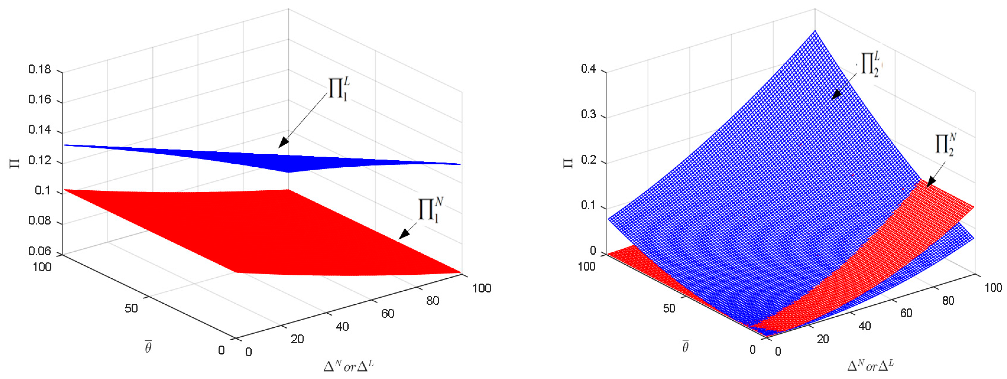
We further analyze the impact of licensing through a numerical example in Figure 2, where and . The results illustrate that when there is no licensing, the profits of the OEM and the IR are independent of the average valuation added to the remanufactured products, denoted as . As the cost saving from remanufacturing increases, the IR’s profit increases and the OEM’s profit decreases. In licensed remanufacturing scenario, however, the IR’s profit increases with and , while the OEM’s profit decreases with and . Moreover, the results show that the OEM can always achieve a higher profit in licensed remanufacturing since the OEM can share in the profits of remanufacturing and has strong market power, even though the existence of remanufactured products will cannibalize the market share of new products. However, this scenario is contingent upon the IR’s acceptance of the OEM’s authorization to remanufacture used products. When is small, the IR will choose to remanufacture used product privately. As increases, the IR becomes increasingly more inclined to cooperate with the OEM.
Proposition 5.
Under the conditions and , the IR will remanufacture used product whether it is licensed by the OEM or not, and the demand for remanufactured products is smaller than the collected quantity of used products. The optimal choice for the OEM and the IR are as follows:
- (i)
- The optimal prices in unlicensed and licensed remanufacturing scenarios are constrained as follows: , while under the condition .
- (ii)
- The optimal quantities are constrained as follows: , while under the condition .
Proposition 5 indicates that the IR will not increase its acquisition price to collect additional used products because , that is, the IR has enough used products to remanufacture to meet the demand, which is different from Proposition 3.
To better describe the impact of licensing on the profits of OEM and IR, we also conduct a numerical analysis as shown in Figure 3, where , , , , and . The result is similar to the example in Figure 2 without licensing. In licensed remanufacturing scenario, however, the profits of the OEM and IR increase with the average valuation added to the remanufactured products and the cost saving from remanufacturing . Moreover, the OEM’s profit is always higher when it chooses to license the IR because it can share the IR’s remanufacturing profit. However, the IR may not accept the OEM’s licensing offer. The result shows that when is sufficiently large, it is more profitable for the IR to choose independent remanufacturing.
Proposition 6.
Under the conditions and , the IR will not engage in remanufacturing regardless of being licensed by the OEM. The optimal decisions of the OEM and the IR are as follows:
- (i)
- The optimal prices in unlicensed and licensed remanufacturing scenarios have the following relationships: .
- (ii)
- The optimal quantities have the following relationships: . Accordingly, .
Proposition 6 indicates that when the IR decides to reclaim used products rather than remanufacture them, the licensing has no impact on IR’s profit, as . However, it is always optimal for the OEM to adopt a licensing strategy if there is competition in collecting used products. The OEM’s profit in licensed remanufacturing scenario is always superior to that in unlicensed remanufacturing scenario. Additionally, the demand of new products will decrease as the OEM increases the sales price of its new products. The IR’s optimal collection strategy does not change with or without licensing because .
Given the fact that in practice many OEMs choose to adopt a licensing strategy, e.g., ZF Friedrichshafen AG cooperates with Xin Meifu and HP works closely with reuse and recycling vendors, there are still many other OEMs that do not know whether to license their remanufacturing business. Through the model discussed above, we can confirm that it is always optimal for the OEM to adopt a licensing strategy if there is competition between OEM’s trade-ins and IR’s collection of used products. On the other hand, it is not necessarily the best for IRs to accept OEM’s authorization.
4.2.2. Comparison of Model L and Model LC
By comparing the results of Model L and Model LC, we can make some observations to understand the role of central coordination in licensed remanufacturing. The results obtained may be helpful for reaching further cooperation between the OEM and the IR. For example, under the premise of authorization, ZF Friedrichshafen AG and Xin Meifu may further cooperate to be a centrally coordinated system, i.e., they may make decisions jointly to achieve a higher total profit.
Proposition 7.
Under the conditions , , and , the IR will engage in remanufacturing and reclaiming, and the demand for remanufactured products is equal to the collected quantity of used products. The optimal decisions of the OEM and the IR are as follows:
- (i)
- The optimal prices have the following relationships: , , under the condition , and under the condition .
- (ii)
- The optimal quantities have the following relationships: while , and under the condition .
- (iii)
- The OEM’s profit has the following relationships: if , for , then ; if , for or , then ; if , for , then . The IR’s profit has the following relationship: under the condition . Where and .
Proposition 7 indicates that unless some specific conditions are met, it is unable to compare the optimal prices, optimal quantities and profits of licensed remanufacturing in a decentralized decision-making system and in a centrally coordinated system, respectively. Moreover, the larger the cost saving from remanufacturing, the more likely the OEM is to make its decision jointly with the IR. For example, if , the OEM’s profit is larger in a centrally coordinated system for . This also applies to the decision of the IR. The larger the cost saving from remanufacturing, the more likely the IR is to be inclined to a centralized decision-making system.
Proposition 8.
Under the conditions and , the IR will remanufacture used products, and the demand for remanufactured products is smaller than the collected quantity of used products. The optimal choices of the OEM and the IR are as follows:
- (i)
- The optimal prices are constrained as follows: , while , , under the condition .
- (ii)
- The optimal quantities are constrained as follows: , , while , under the condition .
- (iii)
- The OEM’s profit has the following relationship: if , for , then ; if , for or , then ; if , for , then . The IR’s profit has the following relationship: if , for , then ; if , for or , then ; if , for , then . Where , and .
Proposition 8 indicates the similar meanings as those in Proposition 7, and there are also some specific conditions have to be met to compare the optimal prices, optimal quantities and profits of the OEM and the IR. Moreover, whether the OEM and the IR make their decisions jointly depends on the cost saving from remanufacturing.
Proposition 9.
Under the conditions and , the IR will not engage in remanufacturing. The optimal decisions of the OEM and the IR are as follows:
- (i)
- The optimal prices have the following relationships: .
- (ii)
- The optimal quantities have the following relationships: , , and . Accordingly, .
Proposition 9 indicates that when the IR decides to reclaim used products rather than remanufacture them, whether the OEM and the IR make decisions jointly or not has no impact on their profits. This means that when the IR only engages in reclaiming used products, a centrally coordinated system makes no sense in terms of CLSC efficiency.
5. Conclusions
In this paper, we focus on unlicensed remanufacturing and licensed remanufacturing strategies in a duopoly market with an OEM and an IR. Based on consumers’ willingness to pay, we develop three models to demonstrate the competition and cooperation between an OEM and an IR. By analyzing the players’ optimal solutions in different scenarios, some interesting findings were obtained.
First, the optimal strategies of the OEM and the IR are influenced by multiple parameters, including the consumer’s valuation of new and remanufactured products, the production cost, and the cost saving from remanufacturing. Both the purchasing decisions and return decisions of consumers will influence the optimal decisions of the OEM and the IR, and when the demand for remanufactured products is low, the IR will alter its remanufacturing and reclaiming strategy.
Second, it is always beneficial for the OEM to choose a licensed remanufacturing strategy because it enables the OEM to share in the profit from the IR’s remanufacturing and decreases the effect of cannibalization. This result seems to be similar to Liu et al.’s [9] finding, namely, the OEM and authorized third party reseller achieve a win-win outcome under some conditions. However, we also find that it is not always profitable for the IR to cooperate with the OEM. When the demand for remanufactured products is low and the benefit of accepting the OEM’s authorization is small, the IR will be willing to remanufacture used products privately. Additionally, being different from Liu et al. [9], we not only help the OEM to decide whether to license its remanufacturing business, but also help the IR to decide whether to accept the OEM authorization.
Third, whether a centrally coordinated system could benefit both the OEM and the IR depends on some specific conditions, especially the cost saving from remanufacturing. A central coordinated system is not necessarily to increase the profits of the OEM and the IR, and has no influence on CLSC efficiency when the IR does not engage in remanufacturing.
These findings can provide a better understanding of a firm’s optimal pricing decisions in various settings and help firms develop more effective operations strategies. However, our models still have several limitations that merit further research. First, we do not consider uncertainty in the collected quantity of used products, which may affect the number of cores available for remanufacturing [40]. Second, we do not consider the quality of used products. In fact, the quality of used products varies and may affect collection and remanufacturing strategies [41]. Third, we use the average valuation added to the remanufactured products to denote the effect of licensing on consumers’ acceptance of remanufactured products. It might be more practical to describe the heterogeneous variation in consumers’ valuation of remanufactured products.
Acknowledgments
This study is supported by National Natural Science Foundation of China (Grant No. 71103149), Humanities and Social Sciences Fund of Ministry of Education (Grant No. 16YJA630005), Major Project of Philosophy and Social Science Research of Sichuan Province (Grant No. SC17A030), Soft Science Research Project of Chengdu City (Grant No. 2016-RK00-00266-ZF), and Chu Tian Scholars Program of Hubei Province.
Author Contributions
Zu-Jun Ma and Ying Dai conceived and designed the study; Qin Zhou and Zu-Jun Ma performed the study and wrote the paper. Ying Dai and Gao-Feng Guan contributed to analysis design and provided advice on the study.
Conflicts of Interest
The authors declare no conflict of interest.
Appendix A
Appendix A.1. Proof of Proposition 1
The decisions faced by the OEM and the IR are given by and , respectively. is strictly concave in and , and is strictly concave in and . The Lagrangian of the IR’s decision problem is . The first-order conditions are , , , and . There are four candidate solutions, which are summarized below:
• Case 1. , which implies .
Solving , , and simultaneously gives , , , and , which further gives , , and .
Therefore, we have if and only if , if and only if , and if and only if .
• Case 2. , which implies .
Solving , , , and simultaneously gives , , , and , which further gives , , and .
Therefore, we have if and only if , if and only if , and if and only if .
• Case 3. , which implies .
Solving , , and simultaneously gives , , , and , which further gives , , , and .
Therefore, we have if and only if , if and only if , and always holds when .
• Case 4. , which can only hold if . This is impossible because it means the unit net value of reclaiming used products is negative. Therefore, this case is ruled out. □
Appendix A.2. Proof of Proposition 2
The decisions faced by the OEM and the IR are given by and , respectively. is strictly concave in , and is strictly concave in . The Lagrangian of the IR’s decision problem is . According to the backward induction method, we consider the optimal pricing decisions and royalty fees. The first-order conditions are , , , and . Substituting these outcomes to can get the optimal solutions. There are four candidate solutions, which are summarized below:
• Case 1. , which implies .
Solving , , , and , and then solving gives , , , , and , which further gives , , and .
Therefore, we have if and only if , if and only if , and if and only if .
• Case 2. , which implies .
Solving , , , and , and then solving gives , , , , and , which further gives , , , and .
Therefore, we have if and only if , if and only if and if and only if .
• Case 3. , which implies .
Solving , , , and , and then solving gives , , , , and , which further gives .
Therefore, we have if and only if , if and only if , and always holds when .
• Case 4. , which can only hold if . This is impossible because it means the unit net value of reclaiming used products is negative. Therefore, this case is ruled out. □
Appendix A.3. Proof of Proposition 3
The decision faced by the OEM and the IR is given by . is strictly concave in . The Lagrangian of the decision problem is . The first-order conditions are , , , and . There are four candidate solutions, which are summarized below:
• Case 1. , which implies .
Solving , , and simultaneously gives , , , and , which further gives , and .
Therefore, we have if and only if , if and only if and if and only if .
• Case 2. , which implies .
Solving , , and simultaneously gives , , , and , which further gives , .
Therefore, we have if and only if , if and only if and if and only if .
• Case 3. , which implies .
Solving , , and simultaneously gives , , , and , which further gives .
Therefore, we have if and only if , if and only if , and always holds when .
• Case 4. , which can only hold if . This is impossible because it means the unit net value of reclaiming used products is negative. Therefore, this case is ruled out. □
Appendix A.4. Proof of Proposition 4
To compare the optimal prices in Model L and Model N in Scenario 1, we have , , and . To solve the roots of and , we have and , respectively.
To compare the optimal quantities in Model L and Model N in Scenario 1, we have and . To solve the roots of and , we have .
Based on the roots, it is easy to prove Proposition 4. □
Appendix A.5. Proof of Proposition 5
To compare the optimal prices in Model L and Model N in Scenario 2, we have , , and . To solve the roots of , we have .
To compare the optimal quantities in Model L and Model N in Scenario 2, we have , , , and . To solve the roots of , we have .
Based on the roots, it is easy to prove Proposition 5. □
Appendix A.6. Proof of Proposition 6
To compare the optimal prices and quantities in Model L and Model N in Scenario 3, we have , , , , , , , and . The difference between the profits is and .□
Appendix A.7. Proof of Proposition 7
To compare the optimal prices in Model LC and Model L in Scenario 1, we have , , and . To solve the roots of and , we have .
To compare the optimal quantities in Model LC and Model L in Scenario 1, we have and . To solve the roots of , and , we have .
To compare the profits in Model LC and Model L in Scenario 1, we have and . To solve the roots of , we have and . To solve the roots of , we have .
Based on the roots, it is easy to prove Proposition 7. □
Appendix A.8. Proof of Proposition 8
To compare the optimal prices in Model LC and Model L in Scenario 2, we have , , and . To solve the roots of , , we have .
To compare the optimal quantities in Model LC and Model L in Scenario 2, we have , , , and . To solve the roots of , , we have .
To compare the profits in Model LC and Model L in Scenario 2, we have and . To solve the roots of , we have and . To solve the roots of , we have and .
Based on the roots, it is easy to prove Proposition 8. □
Appendix A.9. Proof of Proposition 9
To compare the optimal prices and quantities in Model LC and Model L in Scenario 3, we have , , , , and . The difference between the profits is and .□
References
- Bazan, E.; Jaber, M.Y.; Zanoni, S. A review of mathematical inventory models for reverse logistics and the future of its modeling: An environmental perspective. Appl. Math. Model. 2016, 40, 4151–4178. [Google Scholar] [CrossRef]
- Ferrer, G.; Swaminathan, J.M. Managing new and remanufactured products. Manag. Sci. 2006, 52, 15–26. [Google Scholar] [CrossRef] [Green Version]
- Geyer, R.; Van Wassenhove, L.N.; Atasu, A. The impact of limited component durability and finite life cycles on remanufacturing profit. Manag. Sci. 2007, 53, 88–100. [Google Scholar] [CrossRef]
- Ayres, R.; Ferrer, G.; Van Leynseele, T. Eco-efficiency, asset recovery and remanufacturing. Eur. Manag. J. 1997, 15, 557–574. [Google Scholar] [CrossRef]
- Ferguson, M.E. Strategic issues in closed-loop supply chains with remanufacturing. In Closed-Loop Supply Chains: New Developments to Improve the Sustainability of Business Practices; Ferguson, M.E., Souza, G.C., Eds.; Auerbach Publications: Boca Raton, FL, USA, 2010; pp. 9–21. [Google Scholar]
- Hauser, W.M.; Lund, R.T. Remanufacturing, Operating Practices and Strategies: Perspectives on the Management of Remanufacturing Businesses in the United States; Research Report; Boston University: Boston, MA, USA, 2008. [Google Scholar]
- Cat Reman. Available online: https://www.caterpillar.com/en/company/brands/cat-reman.html (accessed on 30 November 2017).
- Stealth Champion of Automatic Gearbox Remanufacturing: Shanghai Xin Fumei. Available online: http://www.xfm960.cn/about/?64.html (accessed on 29 November 2017).
- Liu, H.; Lei, M.; Huang, T.; Leong, G.K. Refurbishing authorization strategy in the secondary market for electrical and electronic products. Int. J. Prod. Econ. 2018, 195, 198–209. [Google Scholar] [CrossRef]
- Atasu, A.; Sarvary, M.; Van Wassenhove, L.N. Remanufacturing as a marketing strategy. Manag. Sci. 2008, 54, 1731–1746. [Google Scholar] [CrossRef]
- Debo, L.G.; Toktay, L.B.; Van Wassenhove, L.N. Market segmentation and product technology selection for remanufacturable products. Manag. Sci. 2005, 51, 1193–1205. [Google Scholar] [CrossRef]
- Heese, H.S.; Cattani, K.; Ferrer, G.; Gilland, W.; Roth, A.V. Competitive advantage through take-back of used products. Eur. J. Oper. Res. 2005, 164, 143–157. [Google Scholar] [CrossRef]
- Wu, C.H. OEM product design in a price competition with remanufactured product. Omega 2013, 41, 287–298. [Google Scholar] [CrossRef]
- Orsdemir, A.; Kemahlıoglu-Ziya, E.; Parlakturk, A.K. Competitive quality choice and remanufacturing. Prod. Oper. Manag. 2014, 23, 48–64. [Google Scholar] [CrossRef]
- Majumder, P.; Groenevelt, H. Competition in remanufacturing. Prod. Oper. Manag. 2001, 10, 125–141. [Google Scholar] [CrossRef]
- Ferguson, M.E.; Toktay, L.B. The effect of competition on recovery strategies. Prod. Oper. Manag. 2006, 15, 351–368. [Google Scholar] [CrossRef]
- Agrawal, V.; Atasu, A.; Van Ittersum, K. Remanufacturing, third-party competition, and consumers’ perceived value of new products. Manag. Sci. 2015, 61, 60–72. [Google Scholar] [CrossRef]
- Wu, X.; Zhou, Y. Does the entry of third-party remanufacturers always hurt original equipment manufacturers? Decis. Sci. 2016, 47, 762–780. [Google Scholar] [CrossRef]
- Wei, S.; Tang, O.; Sundin, E. Core (product) acquisition management for remanufacturing: A review. J. Remanuf. 2015, 5, 1–27. [Google Scholar] [CrossRef]
- Gönsch, J. Buying used products for remanufacturing: Negotiating or posted pricing. J. Bus. Econ. 2014, 84, 715–747. [Google Scholar] [CrossRef]
- Kleber, R.; Zanoni, S.; Zavanella, L. On how buyback and remanufacturing strategies affect the profitability of spare parts supply chains. Int. J. Prod. Econ. 2011, 133, 135–142. [Google Scholar] [CrossRef]
- Ma, Z.J.; Zhou, Q.; Dai, Y.; Sheu, J.B. Optimal pricing decisions under the coexistence of “trade old for new” and “trade old for remanufactured” programs. Transp. Res. Part E 2017, 106, 337–352. [Google Scholar] [CrossRef]
- Klemperer, P. Markets with consumer switching costs. Q. J. Econ. 1987, 102, 375–394. [Google Scholar] [CrossRef]
- Klemperer, P. Welfare Effects of Entry into Markets with Switching Costs. J. Ind. Econ. 1988, 37, 159–165. [Google Scholar] [CrossRef]
- Levinthal, D.A.; Purohit, D. Durable goods and product obsolescence. Mark. Sci. 1989, 8, 35–56. [Google Scholar] [CrossRef]
- Ackere, A.V.; Reyniers, D.J. A rationale for trade-ins. J. Econ. Bus. 1993, 45, 1–16. [Google Scholar] [CrossRef]
- Ackere, A.V.; Reyniers, D.J. Trade-ins and introductory offers in a monopoly. RAND J. Econ. 1995, 26, 58–74. [Google Scholar] [CrossRef]
- Ray, S.; Boyaci, T.; Aras, N. Optimal prices and trade-in rebates for durable, remanufacturable products. Manuf. Serv. Oper. Manag. 2005, 7, 208–228. [Google Scholar] [CrossRef]
- Okada, E.M. Trade-ins, mental accounting, and product replacement decisions. J. Consum. Res. 2001, 27, 433–446. [Google Scholar] [CrossRef]
- Rao, R.S. Understanding the role of trade-ins in durable goods markets: Theory and evidence. Mark. Sci. 2009, 28, 950–967. [Google Scholar] [CrossRef]
- Agrawal, V.V.; Ferguson, M.; Souza, G.C. Trade-in rebates for price discrimination and product recovery. IEEE Trans. Eng. Manag. 2016, 63, 326–339. [Google Scholar] [CrossRef]
- Kaufmann, P.J.; Dant, R.P. The pricing of franchise rights. J. Retail. 2002, 77, 537–545. [Google Scholar] [CrossRef]
- Shane, S.; Shankar, V.; Aravindakshan, A. The effects of new franchisor partnering strategies on franchise system size. Manag. Sci. 2006, 52, 773–787. [Google Scholar] [CrossRef]
- Lal, R. Improving channel coordination through franchising. Mark. Sci. 1990, 9, 299–318. [Google Scholar] [CrossRef]
- Subramanian, R.; Subramanyam, R. Key Factors in the Market for Remanufactured Products. Manuf. Serv. Oper. Manag. 2012, 14, 315–326. [Google Scholar] [CrossRef]
- Zhu, X.; Wang, M.; Chen, G.; Chen, X. The effect of implementing trade-in strategy on duopoly competition. Eur. J. Oper. Res. 2016, 248, 856–868. [Google Scholar] [CrossRef]
- Yin, R.; Tang, C.S. Optimal temporal customer purchasing decisions under trade-in programs with up-front fees. Decis. Sci. 2014, 45, 373–400. [Google Scholar] [CrossRef]
- Chiang, W.Y.K.; Chhajed, D.; Hess, J.D. Direct marketing, indirect profits: A strategic analysis of dual-channel supply-chain design. Manag. Sci. 2003, 49. [Google Scholar] [CrossRef]
- Souza, G.C. Closed-loop supply chains: A critical review, and future research. Decis. Sci. 2013, 44, 7–38. [Google Scholar] [CrossRef]
- Guide, V.D.R.; Wassenhove, L.N. Managing product returns for remanufacturing. Prod. Oper. Manag. 2001, 10, 142–155. [Google Scholar] [CrossRef]
- Guide, V.D.R. Production planning and control for remanufacturing: Industry practice and research needs. J. Oper. Manag. 2000, 18, 467–483. [Google Scholar] [CrossRef]
Figure 1.
Closed-loop supply chain (CLSC) models in licensed and unlicensed remanufacturing scenarios.
Figure 1.
Closed-loop supply chain (CLSC) models in licensed and unlicensed remanufacturing scenarios.
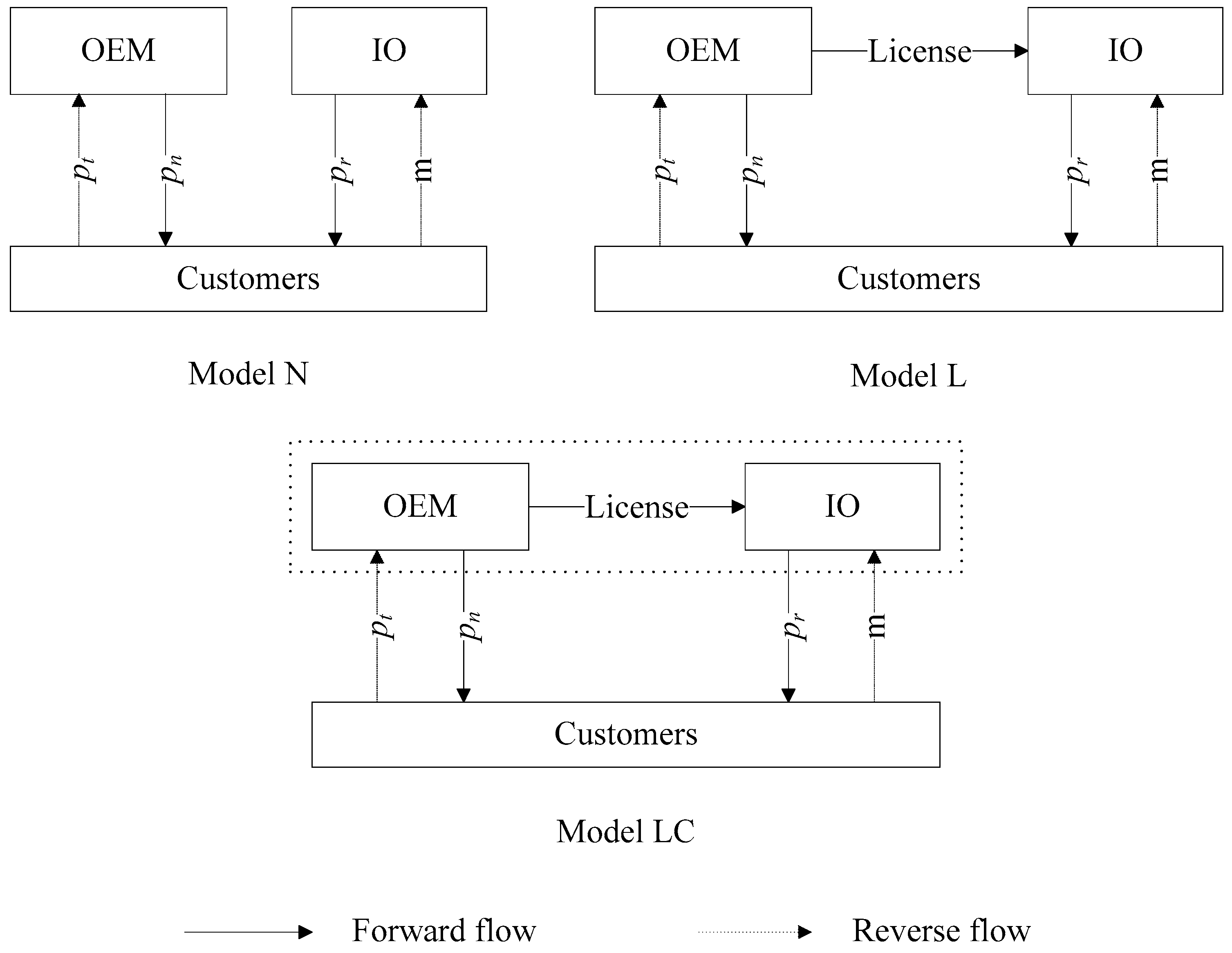
Figure 2.
Effect of and or on the profits of OEM and IR when .

Figure 3.
Effect of and or on the profits of OEM and IR when .


Table 1.
Notations.
| Notations | Definitions |
|---|---|
| Parameters | |
| Total demand for new products | |
| Total demand for remanufactured products | |
| Total demand of trade-in consumers | |
| Total demand of direct-collection consumers | |
| Fraction rate of consumer valuation on remanufactured products, | |
| Durability parameter of new products, | |
| Average increment of consumer’s valuation of licensed remanufactured products | |
| Segment size of customers who hold used products | |
| Unit production cost of new products | |
| Unit cost saving from remanufacturing used products in unlicensed and licensed scenarios respectively () | |
| Unit royalty fee paid by the IR to the OEM for the production and sales of remanufactured products | |
| Unit net value of reclaiming used products for the OEM and the IR respectively, and | |
| Decision Variables | |
| Unit price of new products | |
| Unit price of remanufactured products | |
| OEM’s unit trade-in rebate | |
| IR’s unit acquisition price of used products |
Table 2.
Equilibrium optimal solutions of Model N.
| Optimal Solutions | Scenario 1: | Scenario 2: | Scenario 3: |
|---|---|---|---|
| , , | , | , | |
Table 3.
Equilibrium optimal solutions of Model L.
| Optimal Solutions | Scenario 1: | Scenario 2: | Scenario 3: |
|---|---|---|---|
| , , | , | , | |
Table 4.
Equilibrium optimal solutions of Model LC.
| Optimal Solutions | Scenario 1: | Scenario 2: | Scenario 3: |
|---|---|---|---|
| , , | , | , | |
© 2018 by the authors. Licensee MDPI, Basel, Switzerland. This article is an open access article distributed under the terms and conditions of the Creative Commons Attribution (CC BY) license (http://creativecommons.org/licenses/by/4.0/).
Share and Cite
MDPI and ACS Style
Ma, Z.-J.; Zhou, Q.; Dai, Y.; Guan, G.-F. To License or Not to License Remanufacturing Business? Sustainability 2018, 10, 347. https://doi.org/10.3390/su10020347
AMA Style
Ma Z-J, Zhou Q, Dai Y, Guan G-F. To License or Not to License Remanufacturing Business? Sustainability. 2018; 10(2):347. https://doi.org/10.3390/su10020347
Chicago/Turabian StyleMa, Zu-Jun, Qin Zhou, Ying Dai, and Gao-Feng Guan. 2018. "To License or Not to License Remanufacturing Business?" Sustainability 10, no. 2: 347. https://doi.org/10.3390/su10020347
Note that from the first issue of 2016, this journal uses article numbers instead of page numbers. See further details here.