Exploring the Strengths and Limits of Strong and Weak Sustainability Indicators: A Case Study of the Assessment of China’s Megacities with EF and GPI


1
Smart City Research Center of Zhejiang Province, Hangzhou Dianzi University, Hangzhou 310012, China
2
Institute of Ecological Planning and Landscape Design, College of Life Sciences, Zhejiang University, Hangzhou 310058, China
Sustainability 2018, 10(2), 349; https://doi.org/10.3390/su10020349
Submission received: 30 December 2017
/
Revised: 21 January 2018
/
Accepted: 24 January 2018
/
Published: 30 January 2018
(This article belongs to the Special Issue Defining and Assessing Landscape and Urban Sustainability: Linking Spatial Patterns, Ecosystems Services, and Human Wellbeing)
Abstract
:The perspective of strong/weak sustainability has a great impact on sustainability assessment. In this study, two most widely used indices, Ecological Footprint (EF) and Genuine Progress Indicator (GPI) for strong and weak sustainability assessment, were employed to evaluate the sustainability of China’s ten megacities between 1978 and 2015. The results showed that the ecological footprint had been enlarged in the past twenty years; while the genuine economic welfare started to increase since 2005. The cities of Xi’an, Chengdu, Chongqing, and Shanghai met the threshold of below 2.5 global hectares for EF/capita, and over 3000 dollars/capita (in 2010 US$) for GPI/capita. By analyzing and comparing the characteristics, the processes and results, and the complementary features of evaluation methods of EF and GPI, the research suggested that: (1) Strong and weak sustainability indicators, with their own pros/cons in sustainability assessment, should be used carefully; (2) Weak sustainability indicators could be analyzed from the perspective of strong sustainability; (3) Strong sustainability indicators need to be developed urgently. The results in this study could guide the selection of sustainability indicators, and help interpret the results of sustainability assessment.
1. Introduction
The “three-pillar” or “triple bottom line” concept of sustainability, namely environmental protection, economic development, and social equity, should be considered simultaneously in sustainable development, which has become a consensus in academia [1,2,3,4]. It is a core issue to coordinate the relationships among environment, economy and society in sustainability, the understanding of which should refer to the perspectives of “strong sustainability” and “weak sustainability” [5,6,7]. The main difference of the two perspectives lies in how to treat the substitutability between natural capital and human-made capital. Weak sustainability permits mutual substitutability between natural capital (e.g., ecosystem and biodiversity) and human-made capital (e.g., human structures). According to weak sustainability, a system is sustainable as long as the total amount of capital stocks is not decreasing, even if the environment degrades. Strong sustainability, however, is believed that these two capitals are complementary and environmental sustainability should be assured. Economic development cannot be sustainable at the cost of environment degradation. Strong sustainability can be further divided into two sub-concepts. One denies substitutability and forbids utilization of ecosystem “no matter how many people are starving” [6], and the other permits substitutability at a certain level. These two sub-concepts, as Daly termed, were called as “absurd strong sustainability” and strong sustainability, respectively [6,8]. Apparently, the notions of strong and weak sustainability have a great impact on understanding and evaluating sustainable development [5,6,9,10,11,12].
In China, 17.9% of the residents lived in urban areas in 1978, half in 2011, 57.35% in 2016, and 77.5% will live in urban areas in 2050 according to the UN’s prospect [13]. During unprecedented urbanization, the development of megacities not only represents the achievements of urbanization in China, but also brings about a myriad of problems [14,15,16,17]. Sustainability assessment, especially the indicator set or index, portrays the performance of environment, economy, and society from different aspects for different purposes. According to the definition proposed by Huang [12], most single composite indices are weak sustainability indices, including City Development Index (CDI), Genuine Progress Indicator (GPI), Genuine Savings (GS), Happy Planet Index (HPI), Human Development Index (HDI), Sustainable Society Index (SSI), and Wellbeing Index (WI). Ecological Footprint (EF), Environmental Performance Index (EPI), and Green City Index (GCI) are strong sustainability indices. Among these sustainability indices, CDI, GPI, GS, HPI, SSI, and WI cover three dimensions (i.e., environment, society, and economy), EF, EPI, and GCI cover environmental and social dimensions, and HDI covers social and economic dimensions [12].
Based on previous review and evaluation experiences [12,14], two most widely used indices were employed, EF for strong sustainability assessment and GPI for weak sustainability assessment, to evaluate the sustainability of ten megacities in China between 1978 and 2015. By comparing the differences of assessment methods and results between EF and GPI in a case study, this research tries to find out differences between strong sustainability and weak sustainability, and explore how to better interpret sustainability assessment results and develop strong and weak sustainability indicators.
2. Materials and Methods
2.1. Selection of Megacities
According to high level of regional representation and data availability, ten megacities were selected in this study, with a municipal district population exceeding five million, as defined in the “Adjust the Criteria of Urban Size (2014) No. 51” released by the Central Committee and State Council, Communist Party of China. The ten megacities are all capital cities, located at four regions of China: Western Region (Chengdu, Chongqing, and Xi’an); Central Region (Wuhan); Eastern Region (Beijing, Guangzhou, Nanjing, Shanghai, and Tianjin); and Northeastern Region (Shenyang) (the location of the ten megacities refer to Huang [14]). Chinese cities, different from North American or European cities, are metropolitan regions, which include both urban and rural areas. In this research, urban population means resident population instead of registered population, because the former better reflects the actual level of the city’s resource consumption and waste emissions.
2.2. Selection of Indicators
GPI measures the economic welfare by adding the benefits and subtracting the costs left out of GDP [18,19]. In this study, the mathematical formulation was adapted from Wen et al. [19,20]. Consumer expenditure was a starting point of GPI calculation. The benefit of economy and society, and the cost of economy, society and environment were adding to (or subtracting from) consumer expenditure. It should be noted that the study calculated Gini coefficients for urban and rural areas separately, because of China’s urban-rural dual land system. EF measures the environmental pressure of resource consumption and waste disposal, and Biocapacity (BC) measures the amount of biologically productive land and sea areas available to bear this environmental pressure [21]. The Global Footprint Network’s accounting framework was employed in this study [22], in which average world yield, carbon emission factor, carbon uptake capacity, equivalence factor, and yield factor were set accordingly. Carbon emission factor was based on the Greenhouse Gas Protocol Tool for Energy Consumption in China [23], and was adjusted according to the parameter of China Energy Statistical Yearbook. Yield factor was adopted at provincial scale [24]. Average world yield, carbon uptake capacity and equivalence factor were set by default values [25,26], namely the world average data. Calculation methods of GPI and EF were stated in detail in Huang [14].
2.3. Data Processing
Social and economic data were mainly derived from each city’s Statistical Yearbook, China City Statistical Yearbook, China Energy Statistical Yearbook, China’s New Urbanization Report, and BP Statistical Review of World Energy. Environmental data were obtained from each city’s Statistical Yearbook, China Statistical Yearbook on Environment and Institute of Geographic Sciences and Natural Resources Research, CAS. It should be noted that land use data (in the years 1980, 1990, 2000, 2005, and 2015) of GPI and BC were from Institute of Geographic Sciences and Natural Resources Research, Chinese Academy of Sciences, instead of from the literature as in Huang [14].
The data were collected from 1978 to 2015. Since 1 December 2012, National Bureau of Statistics of China have initiated “Reform of Urban and Rural Household Survey”, which unifies the name, classification and statistical standard of urban and rural residents’ income. Hence, in general, the urban and rural residents’ income data, expenditure data, and consumption data after 2012 should not be compared to the previous data. The execution efficiency of this reform, however, was quite different among cities. Most megacities executed it in 2013 or 2014. Since the data from the new statistic caliber were limited, the data from old caliber were used in this research (Table 1).
To find out the contribution of each indicator to indices (EF and GPI), the study input the indicators of the period (Table 1) to SPSS 20, adopted stepwise linear regression, chose the proper model by t value and significance, and judged the contribution by standardized coefficient in this research.
3. Results
3.1. EF and BC
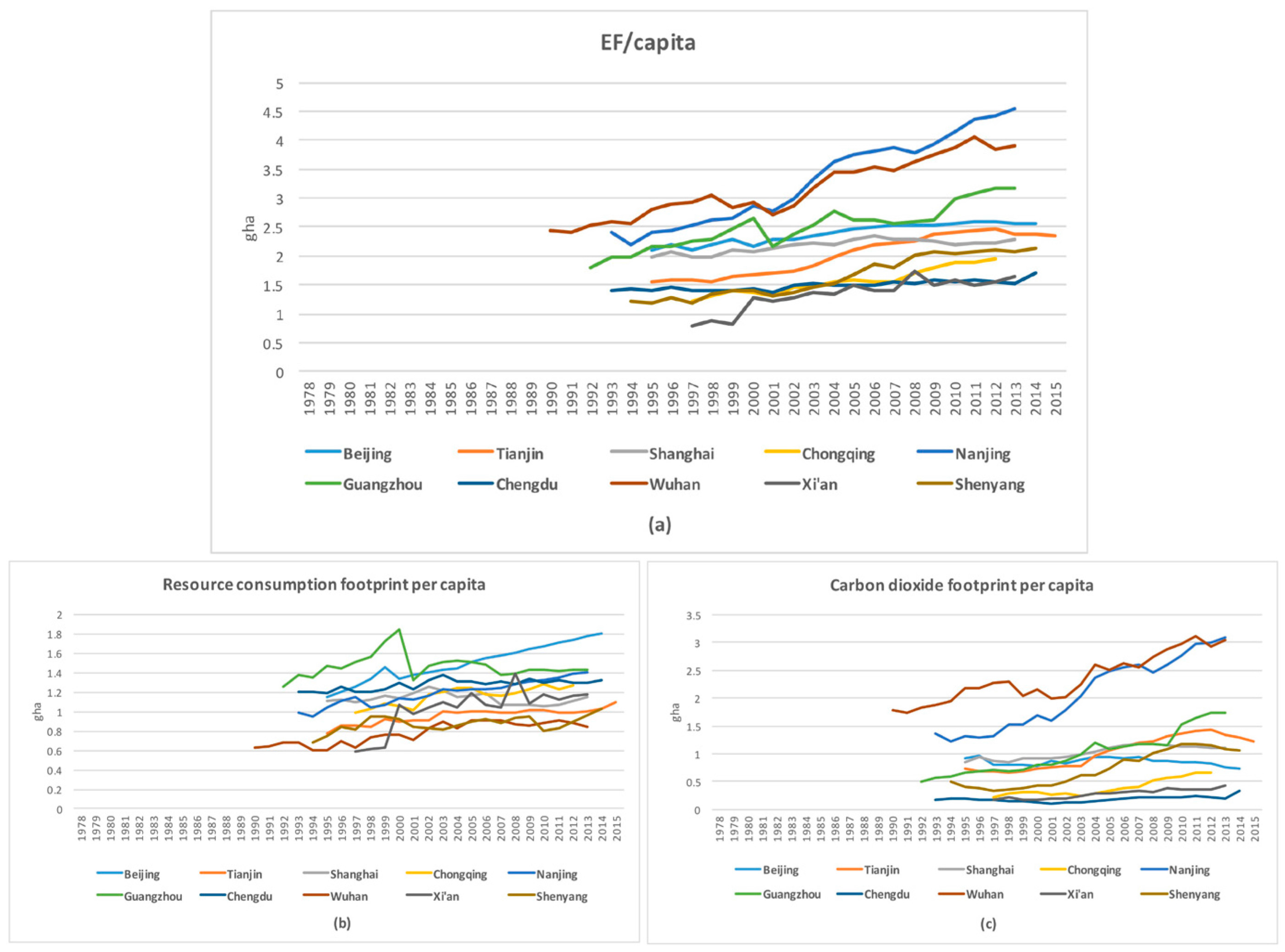
EF/capita of the ten megacities has increased significantly in the past twenty years (Figure 1a). The values of EF/capita for Nanjing and Wuhan were between 3.8 and 4.5 global hectares (gha) after 2010; the values for Guangzhou, Beijing, Tianjin, Shanghai and Shenyang were between 2 and 3 gha; and the values for Chongqing, Xi’an and Chengdu were below 2 gha. Three Western cities performed better than other cities in terms of EF/capita. The value of EF/capita of Chongqing increased remarkably after 2007, and the most stable cities were Chengdu and Xi’an. Among the components of EF, biological resource consumption (namely the cropland footprint, grazing footprint, forest footprint and fishing footprint) increased in general (Figure 1b). Except for Beijing, the values of biological resource consumption of other cities were between 0.8 and 1.4 gha in recent ten years. The biggest increase in CO2 footprint occurred in Nanjing and Wuhan, whose values of CO2 footprint were over 3 gha/capita in 2013 (Figure 1c). The values of Chengdu and Xi’an, however, remained steadily below 0.5 gha.
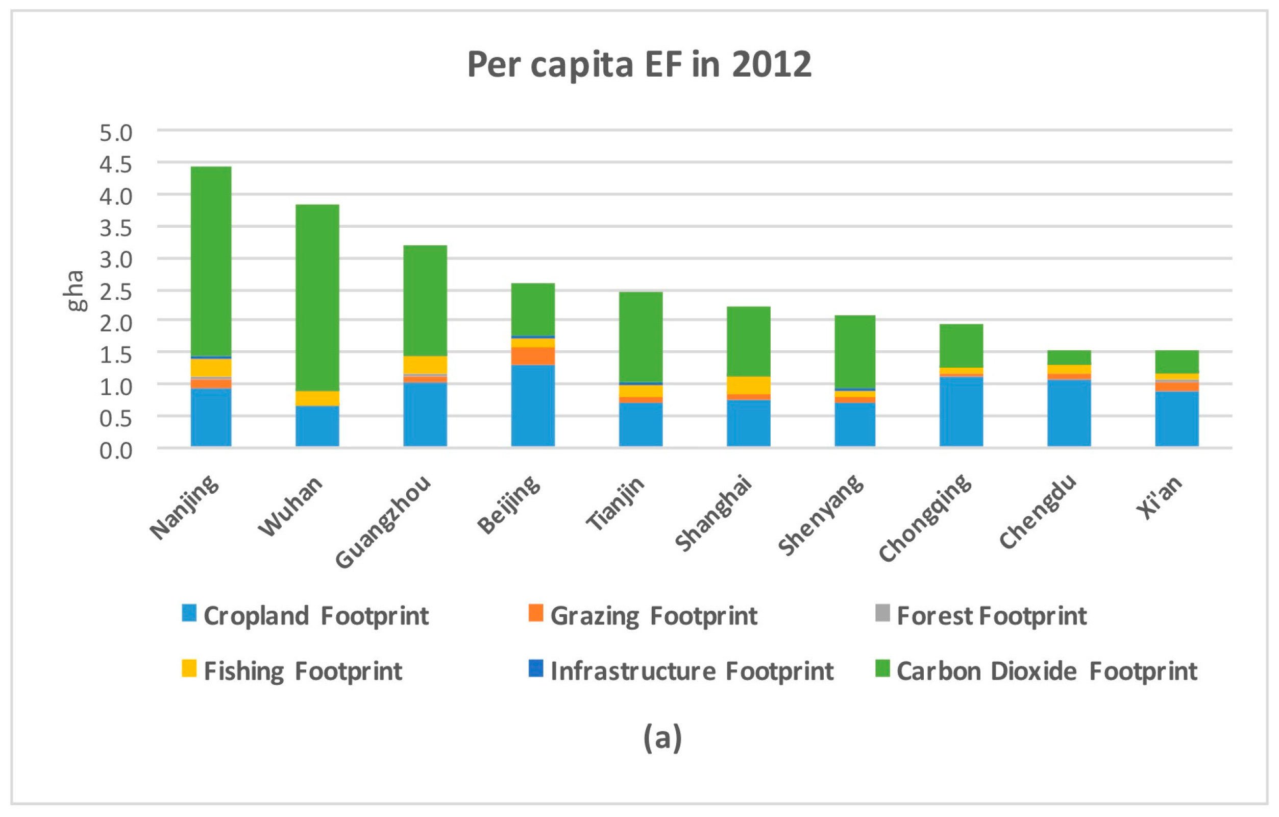
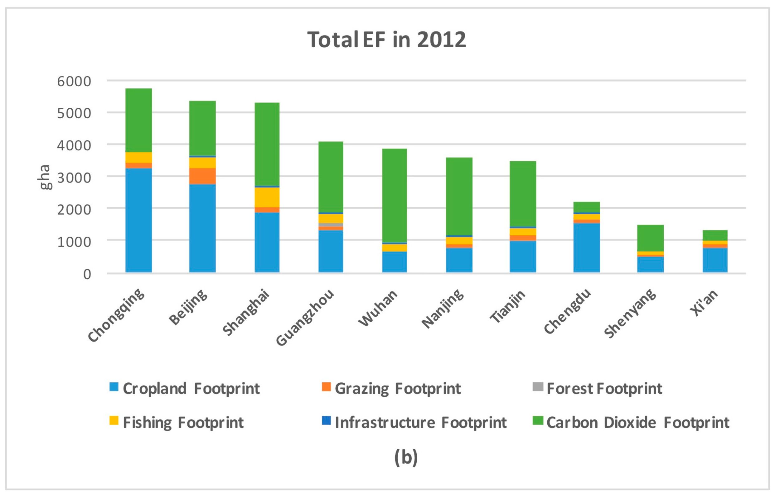
In 2012 (the latest year that all megacities had data), the values of EF/capita varied among ten cities (Figure 2a). The highest value was 4.4 gha (Nanjing), and the lowest was 1.5 gha (Xi’an and Chengdu). Ranking cities by EF, which was quite different from ranking them by EF/capita, Chongqing, Beijing and Shanghai were the top three, and Shenyang and Xi’an were the bottom two (Figure 2b). CO2 footprint contributed most in EF/capita, followed by cropland footprint, fishing footprint, grazing footprint and forest footprint, successively (Table 2). After adding resident population, CO2 footprint and cropland footprint contributed most in EF, followed by fishing footprint, grazing footprint and forest footprint (Table 3).
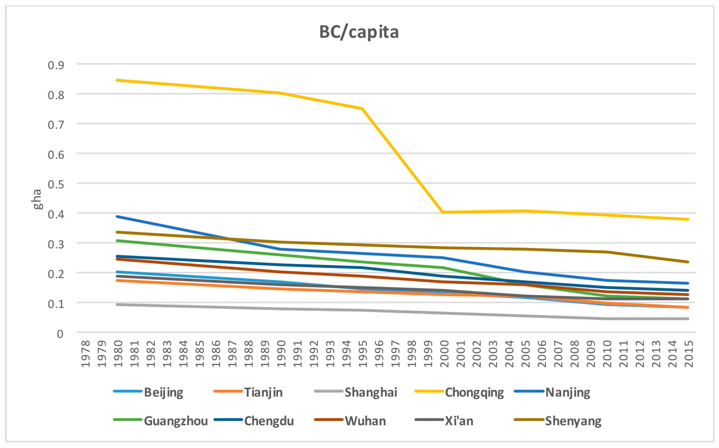
BC/capita varied among cities (Figure 3). The highest value of BC/capita was 0.84 gha (Chongqing) in 1980, and the value dropped to 0.40 gha in 2000. The biocapacity of other cities all decreased from 1980 to 2015, but not as much as that of Chongqing. The ranking order of cities by BC/capita from large to small in 2015 was as follows: Chongqing, Shenyang, Nanjing, Chengdu, Wuhan, Guangzhou, Xi’an, Tianjin, Beijing, and Shanghai. The values of BC/capita in most cities were between 0.1 and 0.3 gha, far lower than that of EF/capita.
3.2. GPI and GDP
GPI/capita and GDP/capita of ten megacities increased in general in the past years, but had different trends (Figure 4a,b). GDP/capita for most cities stabilized (except for the significant decrease in Shanghai from 1980 to 1986) before 1994, and increased dramatically after 1994 (Figure 4b). Different from GDP/capita, GPI/capita stabilized between the year 1994 and the year around 2005, and increased after the year around 2005 (Figure 4a). In the past twenty years, the ratio of GPI to GDP became smaller (Figure 4c). However, the ratio stopped decreasing in recent years. The ratio of some megacities even started to increase slightly. For example, the ratio of Beijing, Shanghai and Shenyang increased in the recent three years.
The performance of GPI/capita in the cities varied in 2012 (Table 4). The smallest value of the ratio of the GPI to GDP was 14.6% (Tianjin), and the largest value was 52.7% (Chongqing). Also, the performance of the components of GPI varied in ten cities. For example, the proportion of economic costs to GPI of Shanghai was 98.7%, and that of Nanjing was 6.8%; the proportion of environmental costs to GPI of Nanjing was 95.0%, and that of Chengdu was 11.7%. The proportion of social benefits to the GPI was large in most cities. The values of the cost of wetland loss and farmland loss were relatively low, and no loss of old-growth forests was observed in ten cities. Among all the twenty indicators, Consumer expenditure contributed most to GPI, followed by Adjustment for unequal income distribution (urban), Value of leisure time, Depletion of nonrenewable resources, and Cost of commuting (Table 5).
3.3. EF and GPI
From the scatterplot of EF/capita and GPI/capita (Figure 5), western cities made progress with relatively low environmental impact. Among the cities of Beijing, Guangzhou and Nanjing, the increasing range of EF/capita in Beijing was the smallest. Even though the value of GPI/capita of Nanjing was large, its value of EF/capita was much larger than the other two cities. Setting threshold of below 2.5 gha for the value of EF/capita, and over 3000 dollars/capita (in 2010 US$) for the value of GPI/capita, only Xi’an (in 2012 and in 2013), Chengdu (in 2013), Chongqing (in 2012), and Shanghai (in 2013) met the threshold.
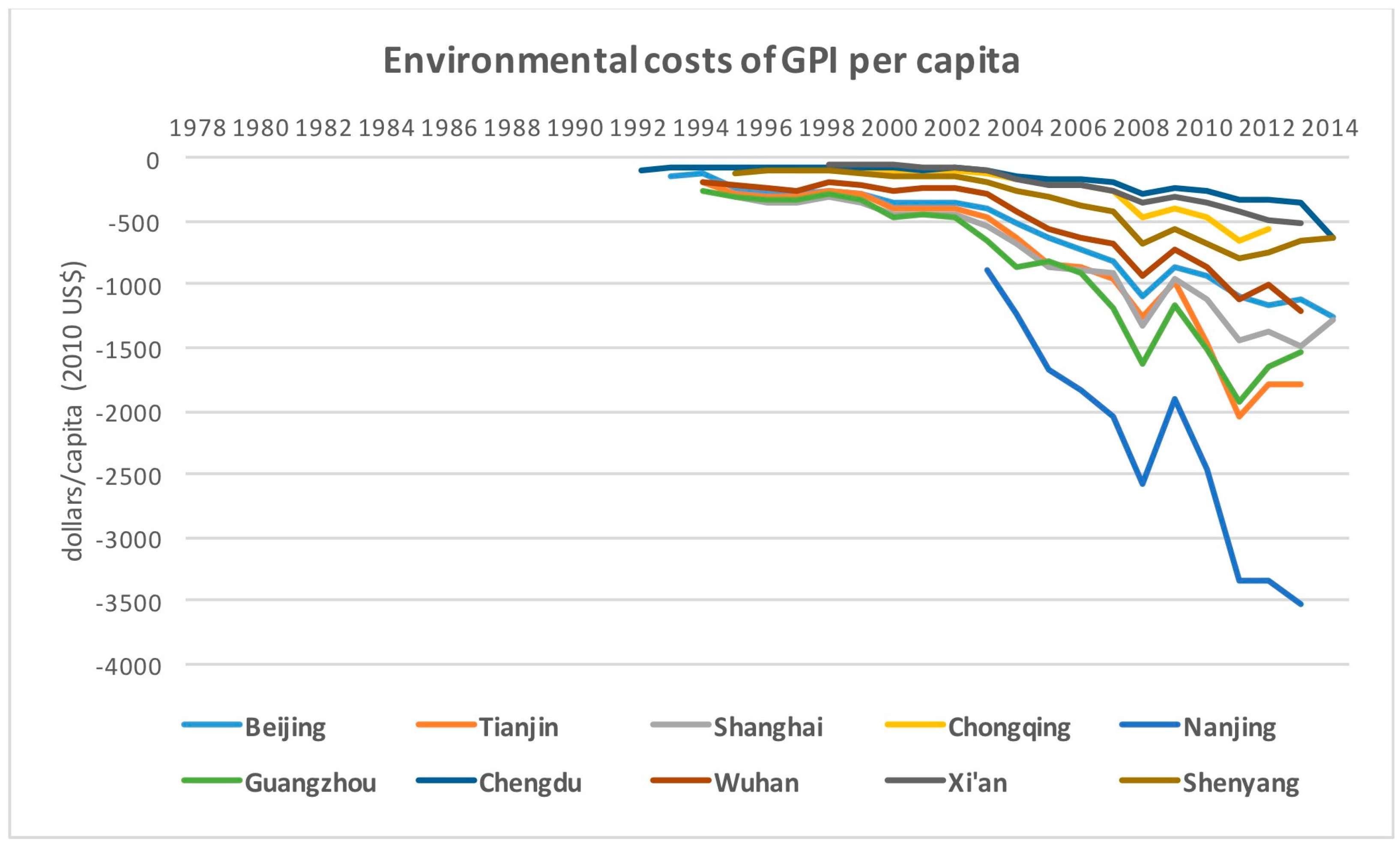
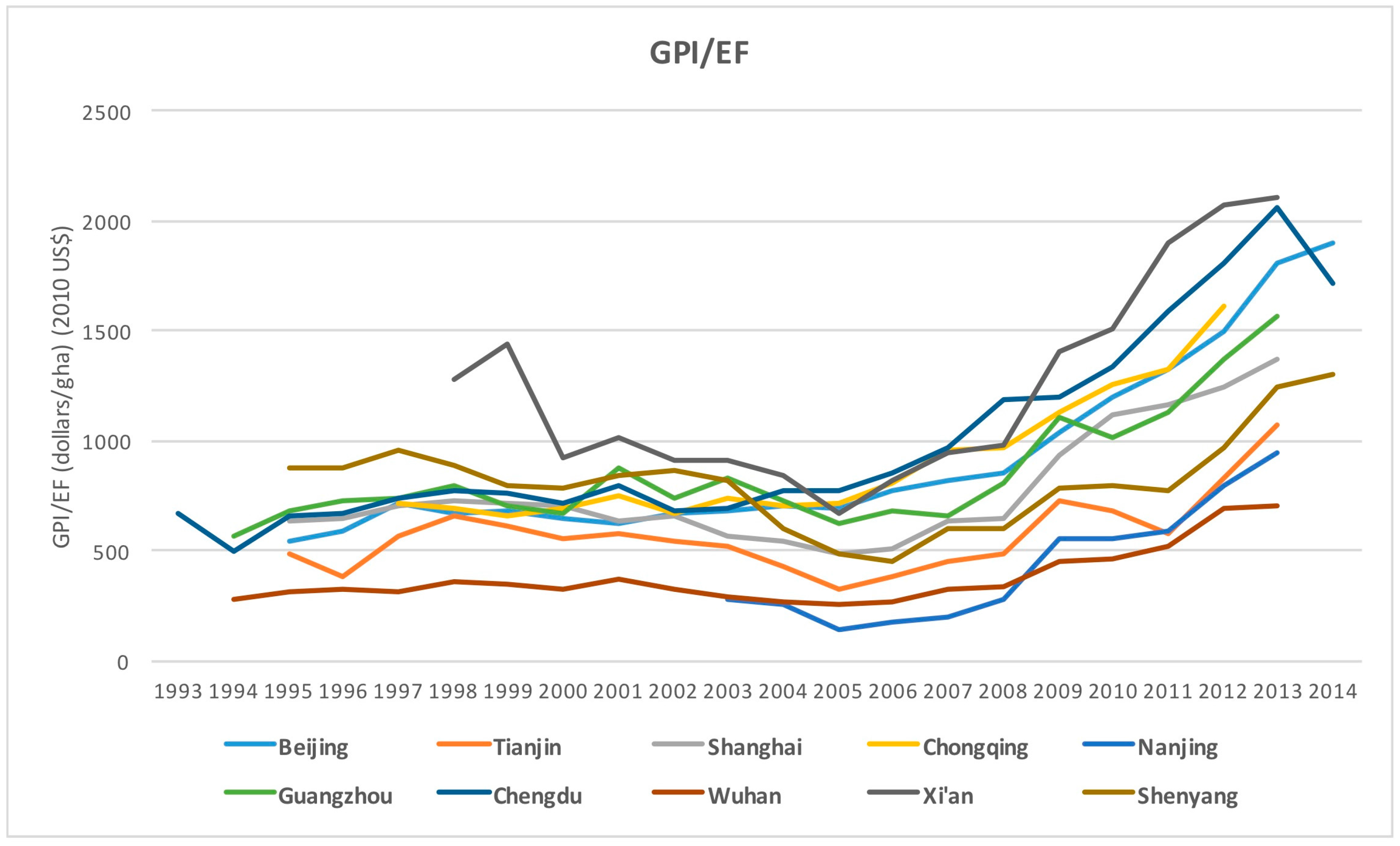
Dividing GPI by EF, namely the genuine economic welfare produced under the pressure of one global hectare of ecological footprint, the value varied dramatically between 140 and 2102 dollars per global hectare (in 2010 US$) (Figure 6). The values of GPI/EF showed an overall declining trend before 2005, and increased significantly after 2005. According to the performance in recent years, the descending order of the megacities in GPI/EF was: Xi’an, Chengdu, Chongqing, Beijing, Guangzhou, Shanghai, Shenyang, Tianjin, Nanjing, and Wuhan. Regarding the environmental costs of GPI per capita and EF/capita, Nanjing performed badly in both of them, and the performances of Chengdu, Xi’an, Chongqing and Shenyang were relatively good in both of them. Wuhan performed badly in EF/capita, while performed well in environmental costs of GPI/capita (Figure 4a and Figure 7).
4. Discussion
4.1. The Differences of Evaluation Processes between EF and GPI
EF is a typical strong sustainability indicator. Its calculation is based on six hypotheses: (1) it is possible to track most resources human consume and most waste human generate; (2) most of these resources and waste can be measured in biologically productive area; (3) all biologically productive areas can be expressed in standardized hectares; (4) standardized hectares can be added up to a total to represent the aggregate human demand; (5) ecological supply can also be expressed in standardized hectares; (6) area demand can exceed area supply, which is called “ecological overshoot” [27].
According to the above hypotheses, the calculation needs average world yield, carbon emission factor, carbon uptake capacity, equivalence factor, and yield factor, all of which have great impact on the result. Theoretically, except for the average world yield, the other four should be set according to the real situation of a particular area (see Section 2.2). If these factors were updated, with the change of biophysical productivity of the particular area and the update of carbon treating technologies, the results of EF would change accordingly. However, dynamic parameters were not available in most situations. Therefore, the trend of EF change, not the result in a particular year, is preferred in assessing urban sustainability.
GPI has been applied at national, regional and urban scales worldwide [14,20,28,29,30,31,32,33]. It should be careful to compare the results from different studies, since the mathematical formulations and data collections of each indicator of GPI might be different among different studies. Three points should be noted in this study: (1) China’s urban-rural dual land system has led to the division of statistical data before and after 2013, so the study calculated Gini coefficients for urban and rural areas separately, instead of the whole city. This problem, however, could be solved using the data after the Reform of Urban and Rural Household Survey; (2) The costs of commuting had increased since 2000 in most cities. For example, the time cost in server congestion and moderate congestion of Beijing reached 90 min daily [34]. This study only calculated time loss of traffic congestion. The cost of extra energy consumption, environmental pollution, traffic accidents and residents’ health should, but have not been included; (3) To calculate the cost of farmland and wetland loss, the total reduced area was multiplied by an annual production and ecological value that could have been provided by the areas if they were not lost. Since the values and the annual reduced areas were relatively small, the costs of farmland loss and wetland loss were small and contributed little to the total GPI (Table 4). Therefore, the value of GPI shows the trend of urban genuine development, but the analysis will be in skin-deep if we do not look into specific indicators of GPI.
4.2. The Differences of Evaluation Results of EF and GPI
The results may be opposite by using EF and GPI to evaluate urban sustainability separately (Figure 1a and Figure 4a). So before the evaluation, it should look into the details of the characteristics of strong and weak sustainability. First, the notions of strong and weak sustainability focus on different aspects. Taking EF and GPI as examples, EF focuses on human impacting on environment, and GPI focuses on ecosystem and environmental state. It noted that multi-dimensional concepts of sustainability may not be considered as fundamentally measuring weak sustainability if equal weights were not assigned to them [12]. The study could analyze the environmental cost of GPI separately. Nanjing and Wuhan were typical cities in this aspect. As both cities performed badly in EF/capita, Wuhan performed relatively better in the environmental cost of GPI/capita than Nanjing did. By analyzing the sub-indicators of GPI, the study found that the main difference between the two cities was the cost of pollution (air pollution was not included), which was lower in Wuhan than in Nanjing. Most indicators of the environmental cost of GPI were calculated by the real cost. Only the cost of pollution was replaced by the investment in environmental infrastructure of the government. Less investment does not necessarily mean healthy environment and ecosystem. If the actual cost of pollution control could be found, the performance of environmental cost of GPI and EF might be consistent.
Second, the interpretations of data were different between EF and GPI. Taking energy consumption and carbon dioxide as examples, EF method could convert carbon dioxide emissions from energy consumption into forest and grazing areas, and GPI calculated the depletion of nonrenewable resources (raw coal, crude oil and natural gas), and the cost of long-term environmental damage by using carbon dioxide and ozone emission data. CO2 footprint contributed most in EF, and depletion of nonrenewable resources contributed relatively high in GPI (the ranking order of standardized coefficients was the fourth when GPI was the dependent variable; and the ranking order was the first when the environmental cost of GPI was the dependent variable). If a city consumes a lot of energy, the performances of EF and GPI will be consistent.
4.3. The Potential to Integrate EF and GPI in Sustainability Assessment
To avoid misleading effect of weak sustainability indicators, researchers suggested to include at least one strong sustainability indicator in the assessment [12]. For example, the ratio of GPI over EF (GPI/EF) could be used as an efficiency indicator for GPI. Happy Planet Index (HPI), a sustainability index covering three dimensions, measures the ecological efficiency with which human wellbeing is delivered [35]. Instead of transferring natural resources into human wellbeing in HPI, GPI/EF converted natural resources into genuine economic development. Wellbeing Index (WI), another widely used index, is special from the perspectives of strong and weak sustainability [36,37]. If the final result of WI is shown by number, it is a weak sustainability index; if it is shown by a two-dimensional graph “Barometer of sustainability”, ecosystem wellbeing and human wellbeing, it is a strong sustainability index. On the barometer, the overall wellbeing is determined by the lower index of ecosystem wellbeing and human wellbeing. Similarly, if a threshold for EF and GPI could be set in the scatterplot, they can be combined as a composite strong sustainability index.
4.4. Suggestions on the Development of Strong/Weak Sustainability Indicators
The notions of strong and weak sustainability have important implications for urban sustainability assessment because they reflect different kinds of sustainability a city intends to achieve. Weak sustainability is not sustainable in the long term. However, weak sustainability indicator can be helpful in communicating with decision-makers and the public at a small scale. Strong sustainability indicator can be used at a large scale, supporting the protection of natural capital. The two could be used simultaneously in real work [5]. However, before weighting and aggregating weak sustainability indicators, the indicators of the index should be analyzed. In addition, it can also adopt multiple methods in 4.3 to analyze weak sustainability indices from the perspective of strong sustainability.
According to this study, it found that EF does not allow for substitutability to a certain degree. So what is the proper threshold to “portray” the degree? “Critical Natural Capital” (CNC) is featured with important environmental functions that could not be provided by human-made capital [10,38]. If we could calculate the amount of the CNC, or even delimit the space covering the CNC, then the degree is clear. To pursue for strong sustainability, it would be ideal to protect the critical natural capital at a large scale, and substitute between natural capital and human-made capital without damaging the CNC at a smaller scale.
5. Conclusions
This study showed that EF of all megacities increased while biocapacity decreased. Three western cities had relatively lower pressures on the environment than other cities did. Carbon dioxide footprint contributed most to EF. The trend of GPI/capita, quite different from GDP/capita, increased after around 2005 after a relatively constant period between 1994 and 2005. Consumer expenditure contributed most to GPI. Only Xi’an, Chengdu, Chongqing and Shanghai met the threshold of below 2.5 gha for the value of EF/capita, and over 3000 dollars/capita (in 2010 US$) for the value of GPI/capita. The performance of the cities varied greatly in terms of the genuine economic welfare produced under the pressure of one global hectare of ecological footprint.
By analyzing and comparing the characteristics, the processes and results, and the complementary features of evaluation methods of EF and GPI, I suggested that: (1) Strong or weak sustainability indicators have their own pros/cons in sustainability assessment and should be used carefully. Strong sustainability is indispensable in sustainability assessment, focusing on the environmental dimension and covering one or two other dimensions. Weak sustainability indicators should be analyzed before weighting and aggregation, and the results of the composite index should be carefully interpreted; (2) Weak sustainability indicators could be analyzed from the perspective of strong sustainability. It is feasible to set threshold for sub-indicators of environmental dimensions, design graphs to outstand the importance of achieving environmental sustainability, and add a strong sustainability indicator to generate a new index; (3) Strong sustainability indicators need to be developed urgently. Critical natural capital is a useful concept to help determine the degree of substitutability between natural capital and human-made capital in number or in space.
Acknowledgments
I would like to thank Jianguo Wu from Arizona State University for his constructive suggestions and revisions. This work was supported by the National Key Research and Development Program of China (No. 2016YFC0502704), and the National Natural Science Foundation of China (No. 41701638).
Conflicts of Interest
The authors declare no conflicts of interest.
References
- National Research Council. Our Common Journey: A Transition Toward Sustainability; National Academy Press: Washington, DC, USA, 1999. [Google Scholar]
- World Commission on Environment and Development (WCED). Our Common Future; Oxford University Press: New York, NY, USA, 1987. [Google Scholar]
- Elkington, J. Enter the triple bottom line. In The Triple Bottom Line: Does It All Add Up? Henriques, A., Richardson, J., Eds.; Earthscan: London, UK, 2004; pp. 1–16. [Google Scholar]
- Kates, R.W.; Clark, W.C.; Corell, R.; Hall, J.M.; Jaeger, C.C.; Lowe, I.; McCarthy, J.J.; Schellnhuber, H.J.; Bolin, B.; Dickson, N.M.; et al. Sustainability Science. Science 2001, 292, 641–642. [Google Scholar] [CrossRef] [PubMed]
- Wu, J.G. Landscape sustainability science: Ecosystem services and human well-being in changing landscapes. Landsc. Ecol. 2013, 28, 999–1023. [Google Scholar] [CrossRef]
- Daly, H.E. On Wilfred Beckerman’s critique of sustainable development. Environ. Values 1995, 4, 49–55. [Google Scholar] [CrossRef]
- Wu, J.G.; Wu, T. Sustainability indicators and indices: An overview. In Handbook of Sustainable Management; Madu, C.N., Kuei, C., Eds.; Imperial College Press: London, UK, 2012; pp. 65–86. [Google Scholar]
- Holland, A. Substitutability: Or, why strong sustainability is weak and absurdly strong sustainability is not absurd. In Valuing Nature? Ethics, Economics and the Environment; Foster, J., Ed.; Routledge: London, UK, 1997; pp. 119–134. [Google Scholar]
- Ekins, P. Environmental sustainability: From environmental valuation to the sustainability gap. Prog. Phys. Geogr. 2011, 35, 629–651. [Google Scholar] [CrossRef]
- Ekins, P.; Simon, S.; Deutsch, L.; Folke, C.; De Groot, R. A framework for the practical application of the concepts of critical natural capital and strong sustainability. Ecol. Econ. 2003, 44, 165–185. [Google Scholar] [CrossRef]
- Wilson, M.C.; Wu, J. The problems of weak sustainability and associated indicators. Int. J. Sustain. Dev. World Ecol. 2017, 24, 44–51. [Google Scholar] [CrossRef]
- Huang, L.; Wu, J.; Yan, L. Defining and measuring urban sustainability: A review of indicators. Landsc. Ecol. 2015, 30, 1175–1193. [Google Scholar] [CrossRef]
- Monitoring Global Population Tends. Available online: https://esa.un.org/unpd/wup/ (accessed on 25 January 2018).
- Huang, L.; Yan, L.; Wu, J. Assessing urban sustainability of Chinese megacities: 35 years after the economic reform and open-door policy. Landsc. Urban Plan. 2016, 145, 57–70. [Google Scholar] [CrossRef]
- Bai, X.M.; Chen, J.; Shi, P.J. Landscape urbanization and economic growth in China: Positive feedbacks and sustainability dilemmas. Environ. Sci. Technol. 2012, 46, 132–139. [Google Scholar] [CrossRef] [PubMed]
- Zhao, S.; Zhou, D.; Zhu, C.; Qu, W.; Zhao, J.; Sun, Y.; Huang, D.; Wu, W.; Liu, S. Rates and patterns of urban expansion in China’s 32 major cities over the past three decades. Landsc. Ecol. 2015, 30, 1541–1559. [Google Scholar] [CrossRef]
- Wu, J.G.; Xiang, W.N.; Zhao, J.Z. Urban ecology in China: Historical developments and future directions. Landsc. Urban Plan 2014, 125, 222–233. [Google Scholar] [CrossRef]
- Kubiszewski, I.; Costanza, R.; Franco, C.; Lawn, P.; Talberth, J.; Jackson, T.; Aylmer, C. Beyond GDP: Measuring and achieving global genuine progress. Ecol. Econ. 2013, 93, 57–68. [Google Scholar] [CrossRef]
- Wen, Z.; Yang, Y.; Lawn, P.A. From GDP to GPI: Quantifying thirty-five years of development in China. In Sustainable Welfare in the Asia-Pacific: Studies Using the Genuine Progress Indicator; Lawn, P.A., Clarke, M., Eds.; Edward Elgar Publishing: Cheltenham, UK, 2008; pp. 228–259. [Google Scholar]
- Wen, Z.; Zhang, K.; Du, B.; Li, Y.; Li, W. Case study on the use of genuine progress indicator to measure urban economic welfare in China. Ecol. Econ. 2007, 63, 463–475. [Google Scholar] [CrossRef]
- Rees, W.; Wackernagel, M. Urban ecological footprints: Why cities cannot be sustainable and why they are a key to sustainability. Environ. Impact Assess. Rev. 1996, 16, 223–248. [Google Scholar] [CrossRef]
- Borucke, M.; Moore, D.; Cranston, G.; Gracey, K.; Iha, K.; Larson, J.; Lazarus, E.; Morales, J.C.; Wackernagel, M.; Galli, A. Accounting for demand and supply of the biosphere’s regenerative capacity: The National Footprint Accounts’ underlying methodology and framework. Ecol. Indic. 2013, 24, 518–533. [Google Scholar] [CrossRef]
- World Resources Institute. Greenhouse Gas Accounting Tool for Chinese Cities (Pilot Version 1.0); World Resources Institute: Beijing, China, 2013. [Google Scholar]
- Liu, M.; Li, W.; Xie, G. Estimation of China ecological footprint production coefficient based on net primary productivity. Chin. J. Ecol. 2010, 29, 592–597. (In Chinese) [Google Scholar]
- Xie, H.Y.; Wang, L.L.; Chen, X.S. Improvement and Application of Ecological Footprint Model, 1st ed.; Chemical Industry Press: Beijing, China, 2008; p. 185. (In Chinese) [Google Scholar]
- Kitzes, J.; Peller, A.; Goldfinger, S.; Wackernagel, M. Current methods for calculating national ecological footprint accounts. Sci. Environ. Sustain. Soc. 2007, 4, 1–9. [Google Scholar]
- Wackernagel, M.; Schulz, N.B.; Deumling, D.; Linares, A.C.; Jenkins, M.; Kapos, V.; Monfreda, C.; Loh, J.; Myers, N.; Norgaard, R.; et al. Tracking the ecological overshoot of the human economy. Proc. Natl. Acad. Sci. USA 2002, 99, 9266–9271. [Google Scholar] [CrossRef] [PubMed]
- Posner, S.M.; Costanza, R. A summary of ISEW and GPI studies at multiple scales and new estimates for Baltimore City, Baltimore County, and the State of Maryland. Ecol. Econ. 2011, 70, 1972–1980. [Google Scholar] [CrossRef]
- Costanza, R.; Erickson, J.; Fligger, K.; Adams, A.; Adams, C.; Altschuler, B.; Balter, S.; Fisher, B.; Hike, J.; Kelly, J.; et al. Estimates of the Genuine Progress Indicator (GPI) for Vermont, Chittenden County and Burlington, from 1950 to 2000. Ecol. Econ. 2004, 51, 139–155. [Google Scholar] [CrossRef]
- Venetoulis, J.; Cobb, C. The Genuine Progress Indicator 1950–2002 (2004 Update); Redefining Progress (RP): San Francisco, CA, USA, 2004. [Google Scholar]
- Zhang, K.; Wen, Z.; Du, B.; Song, G. A multiple-indicators approach to monitoring urban sustainable development. In Ecology, Planning and Management of Urban Forests: International Perspectives; Springer: New York, NY, USA, 2008; pp. 35–52. [Google Scholar]
- Anielski, M.; Johannessen, H. The Edmonton 2008 Genuine Progress Indicator Report; Anielski Management Inc.: Edmonton, AB, Canada, 2009. [Google Scholar]
- Maryland Genuine Progress Indicator. Available online: http://dnr.maryland.gov/mdgpi/Pages/default.aspx (accessed on 25 January 2018).
- Beijing Traffic Development Research Center. 2013 Beijing Transport Annual Report; Beijing Traffic Development Research Center: Beijing, China, 2013. [Google Scholar]
- Abdallah, S.; Thompson, S.; Michaelson, J.; Marks, N.; Steuer, N. The Happy Planet Index 2.0; New Econcomics Foundation: London, UK, 2009. [Google Scholar]
- Prescott-Allen, R. Barometer of sustainability. In Sustainability Indicators: A Report on the Project on Indicators of Sustainable Development; Moldan, B., Billharz, S., Matravers, R., Eds.; Wiley: Chichester, UK, 1997; pp. 133–137. [Google Scholar]
- Prescott-Allen, R. The Wellbeing of Nations: A Country-by-Country Index of Quality of Life and the Environment; Island Press: Washington, DC, USA, 2001. [Google Scholar]
- Pelenc, J.; Ballet, J. Strong sustainability, critical natural capital and the capability approach. Ecol. Econ. 2015, 112, 36–44. [Google Scholar] [CrossRef]
Figure 1.
Temporal dynamics of EF/capita (a), resource consumption footprint per capita (b), and carbon dioxide footprint per capita (c) for the ten megacities.
Figure 1.
Temporal dynamics of EF/capita (a), resource consumption footprint per capita (b), and carbon dioxide footprint per capita (c) for the ten megacities.

Figure 2.
Per capita EF (a) and the total EF (b) in 2012.


Figure 3.
Temporal dynamics of BC/capita for the ten megacities.

Figure 4.
Temporal dynamics of GPI/capita (a), GDP/capita (b), and the ratio of GPI to GDP (c) during 1978 to 2015. GPI/capita and GDP/capita were in 2010 US$.
Figure 4.
Temporal dynamics of GPI/capita (a), GDP/capita (b), and the ratio of GPI to GDP (c) during 1978 to 2015. GPI/capita and GDP/capita were in 2010 US$.
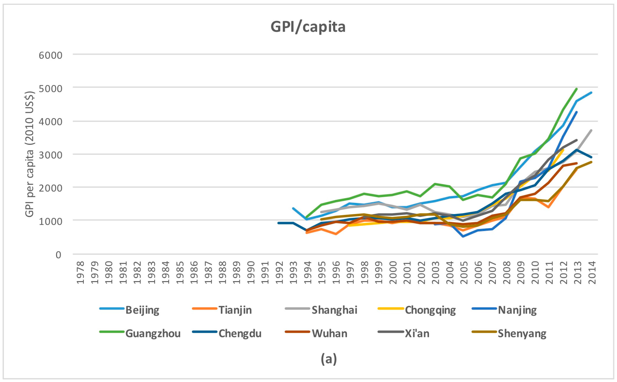

Figure 5.
Scatterplot of EF/capita and GPI/capita for ten megacities. GPI/capita was in 2010 US$.
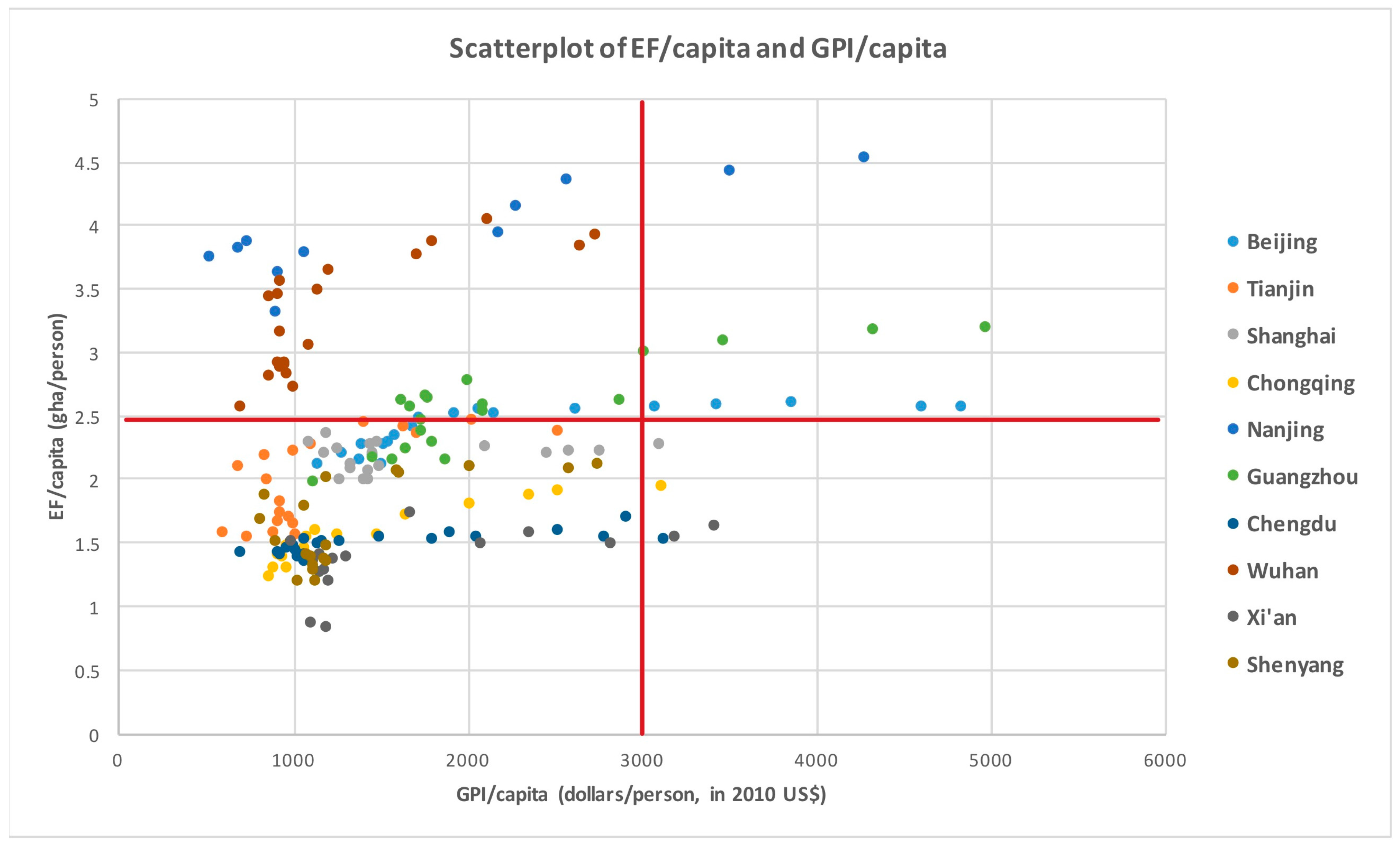
Figure 6.
Temporal dynamics of the ratio of GPI to EF for ten megacities.

Figure 7.
Temporal dynamics of environmental costs of GPI for ten megacities.

Table 1.
The starting and ending year of indices of data collection. The starting year: according to data availability; the ending year: using the data from old statistic caliber according to the “Reform of Urban and Rural Household Survey”.
Table 1.
The starting and ending year of indices of data collection. The starting year: according to data availability; the ending year: using the data from old statistic caliber according to the “Reform of Urban and Rural Household Survey”.
| Region | Megacity | Starting-Ending Year of EF | Starting-Ending Year of GPI |
|---|---|---|---|
| Eastern region | Beijing | 1995–2014 | 1993–2014 |
| Tianjin | 1995–2015 | 1994–2013 | |
| Nanjing | 1993–2013 | 2003–2013 | |
| Shanghai | 1995–2013 | 1995–2014 | |
| Guangzhou | 1992–2013 | 1994–2013 | |
| Western region | Chongqing | 1997–2012 | 1997–2012 |
| Chengdu | 1993–2014 | 1992–2014 | |
| Xi’an | 1997–2013 | 1998–2013 | |
| Middle region | Wuhan | 1990–2013 | 1994–2013 |
| Northeastern region | Shenyang | 1994–2014 | 1995–2014 |
Table 2.
The coefficients of stepwise linear regression. EF/capita was the dependent variable for cropland footprint, grazing footprint, fishing footprint, forest footprint, carbon dioxide footprint, infrastructure footprint (per capita), and population.
Table 2.
The coefficients of stepwise linear regression. EF/capita was the dependent variable for cropland footprint, grazing footprint, fishing footprint, forest footprint, carbon dioxide footprint, infrastructure footprint (per capita), and population.
| Unstandardized Coefficients | Standardized Coefficients | t | Significance | ||
|---|---|---|---|---|---|
| B | Std. Error | Beta | |||
| Constant | 0.046 | 0.003 | 13.426 | 0.000 | |
| Carbon Dioxide Footprint | 1.001 | 0.001 | 1.014 | 957.455 | 0.000 |
| Cropland Footprint | 0.966 | 0.004 | 0.266 | 258.096 | 0.000 |
| Fishing Footprint | 0.989 | 0.010 | 0.114 | 99.594 | 0.000 |
| Grazing Footprint | 1.162 | 0.013 | 0.083 | 86.639 | 0.000 |
| Forest Footprint | 1.079 | 0.026 | 0.044 | 41.444 | 0.000 |
Table 3.
The coefficients of stepwise linear regression. EF was the dependent variable for cropland footprint, grazing footprint, fishing footprint, forest footprint, carbon dioxide footprint, infrastructure footprint (total values), and population.
Table 3.
The coefficients of stepwise linear regression. EF was the dependent variable for cropland footprint, grazing footprint, fishing footprint, forest footprint, carbon dioxide footprint, infrastructure footprint (total values), and population.
| Unstandardized Coefficients | Standardized Coefficients | t | Significance | ||
|---|---|---|---|---|---|
| B | Std. Error | Beta | |||
| Constant | 22.920 | 1.188 | 19.299 | 0.000 | |
| Carbon Dioxide Footprint | 0.999 | 0.001 | 0.578 | 1092.358 | 0.000 |
| Cropland Footprint | 0.995 | 0.001 | 0.569 | 1104.422 | 0.000 |
| Fishing Footprint | 1.032 | 0.006 | 0.106 | 181.290 | 0.000 |
| Grazing Footprint | 1.115 | 0.007 | 0.081 | 161.084 | 0.000 |
| Forest Footprint | 0.898 | 0.023 | 0.017 | 39.139 | 0.000 |
Table 4.
GPI/capita and its components among the ten megacities in 2012. The unit was dollar (in 2010 US$) or specified otherwise. Blank spaces were missing values.
Table 4.
GPI/capita and its components among the ten megacities in 2012. The unit was dollar (in 2010 US$) or specified otherwise. Blank spaces were missing values.
| Beijing | Tianjin | Shanghai | Chongqing | Nanjing | Guangzhou | Chengdu | Wuhan | Xi’an | Shenyang | ||
|---|---|---|---|---|---|---|---|---|---|---|---|
| GPI’s starting point | Consumer expenditure | 4568.7 | 3430.3 | 5583.7 | 2072.0 | 4434.8 | 5761.7 | 2506.5 | 2639.2 | 2873.3 | 3303.0 |
| Economy | Adjustment for unequal income distribution-Rural | 0.0 | 0.0 | 0.0 | 0.0 | ||||||
| Adjustment for unequal income distribution-Urban | −1567.9 | −1380.6 | −2619.1 | −315.6 | 0.0 | −1307.8 | −666.6 | −508.1 | −830.1 | −1137.6 | |
| Cost of consumer durables | −94.8 | −79.5 | −101.9 | −131.0 | −237.3 | −108.5 | −74.4 | −79.9 | −104.3 | −165.2 | |
| Economic costs-Proportion to GPI (%) | −43.0 | −72.0 | −98.7 | −14.3 | −6.8 | −32.7 | −26.6 | −22.2 | −29.3 | −64.6 | |
| Services of consumer durables | 426.5 | 357.9 | 458.7 | 589.4 | 1067.9 | 488.4 | 334.8 | 359.5 | 469.4 | 743.5 | |
| Economic benefits-Proportion to GPI (%) | 11.0 | 17.6 | 16.6 | 18.9 | 30.4 | 11.3 | 12.0 | 13.6 | 14.7 | 36.8 | |
| Society | Cost of crime | −75.2 | 120.7 | −141.5 | −73.1 | −91.5 | −126.2 | −64.9 | −83.5 | −58.2 | −86.2 |
| Cost of automobile accidents | −0.2 | −0.4 | −0.1 | −0.1 | −0.1 | −0.1 | −0.1 | −0.2 | −0.1 | ||
| Cost of commuting | −685.8 | −569.1 | −528.8 | −111.8 | −306.7 | −718.2 | −265.1 | −136.9 | −235.8 | −546.0 | |
| Cost of family breakup | −2.9 | −2.2 | −2.7 | −2.6 | −2.7 | −2.0 | −3.2 | −2.4 | −2.0 | −3.1 | |
| Cost of underemployment | −4.7 | −20.9 | −18.3 | −5.7 | −7.3 | −29.8 | −13.5 | −10.9 | −13.8 | −11.3 | |
| Social costs-Proportion to GPI (%) | −19.9 | −23.3 | −25.1 | −6.2 | −11.6 | −20.2 | −12.4 | −8.8 | −9.7 | −32.0 | |
| Value of leisure time | 2191.9 | 1678.7 | 1266.8 | 1208.7 | 1704.2 | 1791.3 | 1027.5 | 1176.0 | 1286.5 | 346.7 | |
| Value of housework and parenting | 250.2 | 252.7 | 223.9 | 421.3 | 267.9 | 209.5 | 320.4 | 282.6 | 284.7 | 318.2 | |
| Value of volunteer work | 26.7 | 20.4 | 15.4 | 14.7 | 20.7 | 21.8 | 12.5 | 14.3 | 15.7 | 4.2 | |
| Social benefits-Proportion to GPI (%) | 63.8 | 96.2 | 54.6 | 52.8 | 56.7 | 46.7 | 48.8 | 55.6 | 49.7 | 33.2 | |
| Environment | Cost of pollution (air pollution is not included) | −252.3 | −169.9 | −85.9 | −96.7 | −501.1 | −25.3 | −49.2 | −23.9 | −25.2 | −13.2 |
| Cost of air pollution | −250.2 | −264.2 | −245.5 | −112.2 | −256.3 | −305.6 | −166.2 | −229.0 | −147.8 | −232.4 | |
| Cost of wetland loss | 0.0 | −0.4 | −0.1 | 0.0 | −0.1 | 0.0 | 0.0 | −0.1 | 0.1 | 0.0 | |
| Cost of farmland loss | −0.4 | −0.8 | −0.7 | −0.6 | −1.0 | −0.4 | −1.4 | −2.1 | −1.9 | −0.7 | |
| Loss of old-growth forests | 0.0 | 0.0 | 0.0 | 0.0 | 0.0 | 0.0 | 0.0 | 0.0 | 0.0 | 0.0 | |
| Depletion of nonrenewable resources | −632.2 | −1304.3 | −1014.3 | −307.7 | −2517.1 | −1269.7 | −93.7 | −688.2 | −305.1 | −470.8 | |
| Cost of long-term environmental damage | −29.2 | −39.2 | −32.9 | −34.8 | −61.5 | −46.3 | −14.6 | −58.7 | −15.3 | −30.8 | |
| Environmental costs-Proportion to GPI (%) | −30.1 | −87.7 | −50.0 | −17.7 | −95.0 | −38.0 | −11.7 | −37.8 | −15.5 | −37.1 | |
| Results | Resident population (10,000) | 2069.3 | 1413.2 | 2380.4 | 2945.0 | 813.5 | 1283.9 | 1417.8 | 1012.0 | 855.3 | 822.8 |
| GPI/capita | 3868.0 | 2029.3 | 2756.9 | 3114.1 | 3513.0 | 4332.8 | 2788.6 | 2647.5 | 3189.8 | 2018.2 | |
| GDP/capita | 13168.2 | 13905.7 | 12921.1 | 5904.5 | 13491.5 | 16085.9 | 8748.9 | 12053.5 | 7779.9 | 12229.7 | |
| GPI/GDP (%) | 29.4 | 14.6 | 21.3 | 52.7 | 26.0 | 26.9 | 31.9 | 22.0 | 41.0 | 16.5 |
Table 5.
The coefficients of stepwise linear regression. GPI/capita was the dependent variable for the twenty sub-indicators of GPI/capita.
Table 5.
The coefficients of stepwise linear regression. GPI/capita was the dependent variable for the twenty sub-indicators of GPI/capita.
| Unstandardized Coefficients | Standardized Coefficients | t | Significance | ||
|---|---|---|---|---|---|
| B | Std. Error | Beta | |||
| Constant | 3.611 | 0.994 | 3.634 | 0.000 | |
| Cost of crime | 1.001 | 0.004 | 0.057 | 247.309 | 0.000 |
| Services of consumer durables | 0.782 | 0.001 | 0.136 | 576.641 | 0.000 |
| Depletion of nonrenewable resources | 0.998 | 0.001 | 0.385 | 1223.785 | 0.000 |
| Cost of underemployment | 1.000 | 0.040 | 0.007 | 25.071 | 0.000 |
| Consumer expenditure | 1.000 | 0.001 | 1.580 | 1601.695 | 0.000 |
| Adjustment for unequal income distribution-Urban | 1.001 | 0.001 | 0.672 | 1478.015 | 0.000 |
| Cost of commuting | 0.996 | 0.002 | 0.241 | 442.321 | 0.000 |
| Value of housework and parenting | 0.981 | 0.003 | 0.057 | 318.043 | 0.000 |
| Cost of pollution | 1.003 | 0.003 | 0.078 | 329.689 | 0.000 |
| Cost of air pollution | 1.030 | 0.007 | 0.094 | 149.287 | 0.000 |
| Loss of leisure time | 1.012 | 0.001 | 0.629 | 1947.977 | 0.000 |
| Adjustment for unequal income distribution-Rural | 1.042 | 0.015 | 0.010 | 71.826 | 0.000 |
| Cost of long term environmental damage | 0.975 | 0.015 | 0.014 | 65.353 | 0.000 |
© 2018 by the author. Licensee MDPI, Basel, Switzerland. This article is an open access article distributed under the terms and conditions of the Creative Commons Attribution (CC BY) license (http://creativecommons.org/licenses/by/4.0/).
Share and Cite
MDPI and ACS Style
Huang, L. Exploring the Strengths and Limits of Strong and Weak Sustainability Indicators: A Case Study of the Assessment of China’s Megacities with EF and GPI. Sustainability 2018, 10, 349. https://doi.org/10.3390/su10020349
AMA Style
Huang L. Exploring the Strengths and Limits of Strong and Weak Sustainability Indicators: A Case Study of the Assessment of China’s Megacities with EF and GPI. Sustainability. 2018; 10(2):349. https://doi.org/10.3390/su10020349
Chicago/Turabian StyleHuang, Lu. 2018. "Exploring the Strengths and Limits of Strong and Weak Sustainability Indicators: A Case Study of the Assessment of China’s Megacities with EF and GPI" Sustainability 10, no. 2: 349. https://doi.org/10.3390/su10020349
Note that from the first issue of 2016, this journal uses article numbers instead of page numbers. See further details here.