Interannual Carbon and Nutrient Fluxes in Southeastern Taiwan Strait


1
Department of Oceanography, National Sun Yat-sen University, Kaohsiung 80424, Taiwan
2
Department of Mathematics and Statistics, Oakland University, Rochester, MI 48309, USA
3
Institute of Marine Environmental Science and Technology, National Taiwan Normal University, Taipei 10610, Taiwan
*
Author to whom correspondence should be addressed.
Sustainability 2018, 10(2), 372; https://doi.org/10.3390/su10020372
Submission received: 2 January 2018
/
Revised: 26 January 2018
/
Accepted: 26 January 2018
/
Published: 31 January 2018
(This article belongs to the Special Issue Marine Carbon Cycles)
Abstract
:The Taiwan Strait (TS) is one of the main sources of phosphate that supports the large fish catches of the phosphate-limited East China Sea (ECS). The Penghu Channel is the deepest part of the TS, and most of the flow of the TS towards the ECS is principally through this channel. Empirical equations that are based on measurements made during 19 cruises (2000–2011) were combined with water velocity, salinity, and temperature, which were modeled using HYCOM (the Hybrid Coordinate Ocean Model) to obtain the annual fluxes for total alkalinity (TA), dissolved inorganic carbon (DIC), nitrate plus nitrite, phosphate, and silicate fluxes. The TA and DIC are mainly transported in the top layer (0–55 m) because the current is much stronger there than in the bottom layer (55–125 m) whereas the TA and DIC concentrations in the top layer are only slightly smaller compared with the bottom layer. In contrast, the nitrate plus nitrite flux is mainly transported in the bottom layer because the concentrations are much higher in the bottom layer. Generally, nutrient flux increases with the Pacific Decadal Oscillation (PDO) index, but TA and DIC fluxes increase as the PDO index decreases.
1. Introduction
The Taiwan Strait (TS) directly connects the South China Sea (SCS) and the East China Sea (ECS), which are two bountiful marginal seas. The three major water masses in the TS are the Minzhe Coastal Water, the surface water of the SCS, and the surface water of the West Philippines Sea (WPS). Generally, the Minzhe Coastal Water has the highest nutrient concentrations among these three water masses, and the surface water of the WPS, which is brought into the TS through Kuroshio intruding the SCS, contains the lowest nutrient concentrations. The TS transports a mixture of SCS water and WPS water to the ECS mostly in the summer, while the Minzhe Coastal Water flows southward along the western side of the TS to the northern SCS in the winter. Through the exchange of water masses, the TS transports nutrients between these two seas [1,2].
The nutrient budgets in the ECS are influenced by fluvial transport, Kuroshio Intermediate Water, and TS seawater [3,4]. The nitrate and phosphate fluxes in the Yangtze River have increased dramatically with the population and consumption of fertilizer in the basin, but the silicon flux is reduced by sediment trapping in reservoirs [5]. The ecosystem in the Yangtze estuary has changed as the number of non-siliceous algae and the red tides of harmful algal blooms have increased because of the varied nutrient concentration ratios [6,7]. The biological uptake ratio between nitrogen and phosphate is around 16:1 in the ocean, and this is called the Redfile ratio. The fluvial transport with extremely high N/P ratio (long term annual averaged N:P ≈ 250:1, [5]) has also caused the ECS to become phosphate-limited, while the other two main water masses of the ECS are nitrogen-limited [8]. Chen and Wang [3] estimated that the TS annually delivers 22.4 × 10⁹ mol year−1 (0.71 kmol s−1), 2.24 × 10⁹ mol year−1 (0.07 kmol s−1) and 56 × 109 mol year−1 (1.78 kmol s−1) of nitrogen, phosphate and silicate to the ECS, and that equal 0.50, 13 and 0.65 times the fluxes of nitrogen (1.41 kmol s−1), phosphate (0.005 kmol s−1) and silicate (2.7 kmol s−1) from the Yangtze River [5]. Liu et al. [9] reported summer nitrate, phosphate, and silicate fluxes in the TS at 1.90 kmol N s−1, 0.25 kmol P s−1, and 8.4 kmol Si s−1, respectively, in August 1994; and winter nitrate, phosphate, and silicate fluxes in the TS of 12.9 kmol N s−1, 0.85 kmol P s−1, and 22.6 kmol Si s−1, respectively, in March 1997. Notably, the values in March might have been significantly overestimated [10]. Chung et al. [11] calculated nitrate and phosphate fluxes in the TS at 0.96 kmol N s−1 and 0.16 kmol P s−1 in May 1999, and 1.82 kmol N s−1 and 0.34 kmol P s−1 in August 1999, based on measurements made during one cruise in that month.
Located in the southeast and deepest part of the TS, the Penghu Channel (PHC) is funnel-shaped and is responsible for 60% of the northward flow [12,13]. The Strait receives southwesterly and northeasterly winds in the summer and winter, respectively, and the water transport in the TS varies with the wind stress [14,15]. The northward transports are highest and lowest in the summer and winter, respectively, and the water flux direction even becomes southward during strong northeasterly winds [16]. The northward transport in the TS contains mixed SCS and WPS seawater, and the mixing percentage varies with the season. In general, the amount of WPS water in the PHC during winter is greater than that in summer [17]; this result reflects the seasonal westward Kuroshio intrusion through the Luzon Strait, which forms the boundary between the SCS and WPS, bringing WPS water into the northern SCS [18].
Along with its seasonal variation, the Kuroshio intrusion is affected by large-scale climate events and climatic patterns, such as El Niño and the Pacific Decadal Oscillation (PDO) [19,20]. The subsurface WPS water is typically warmer, saltier and more oligotrophic than the subsurface SCS water in the similar layer [1,21]. Accordingly, the nutrient and carbon concentrations of the seawater in the PHC vary with the ratio of the amounts of the different seawaters. However, the interannual and seasonal interactions among nutrient flux, inorganic carbon flux, the biological effects, and the water flux are still unknown. This investigation concerns the interannual and seasonal nutrient and inorganic carbon fluxes. It also provides a mathematical method to synthesize long-term averaged chemical concentrations to estimate chemical fluxes in the PHC.
2. Materials and Methods
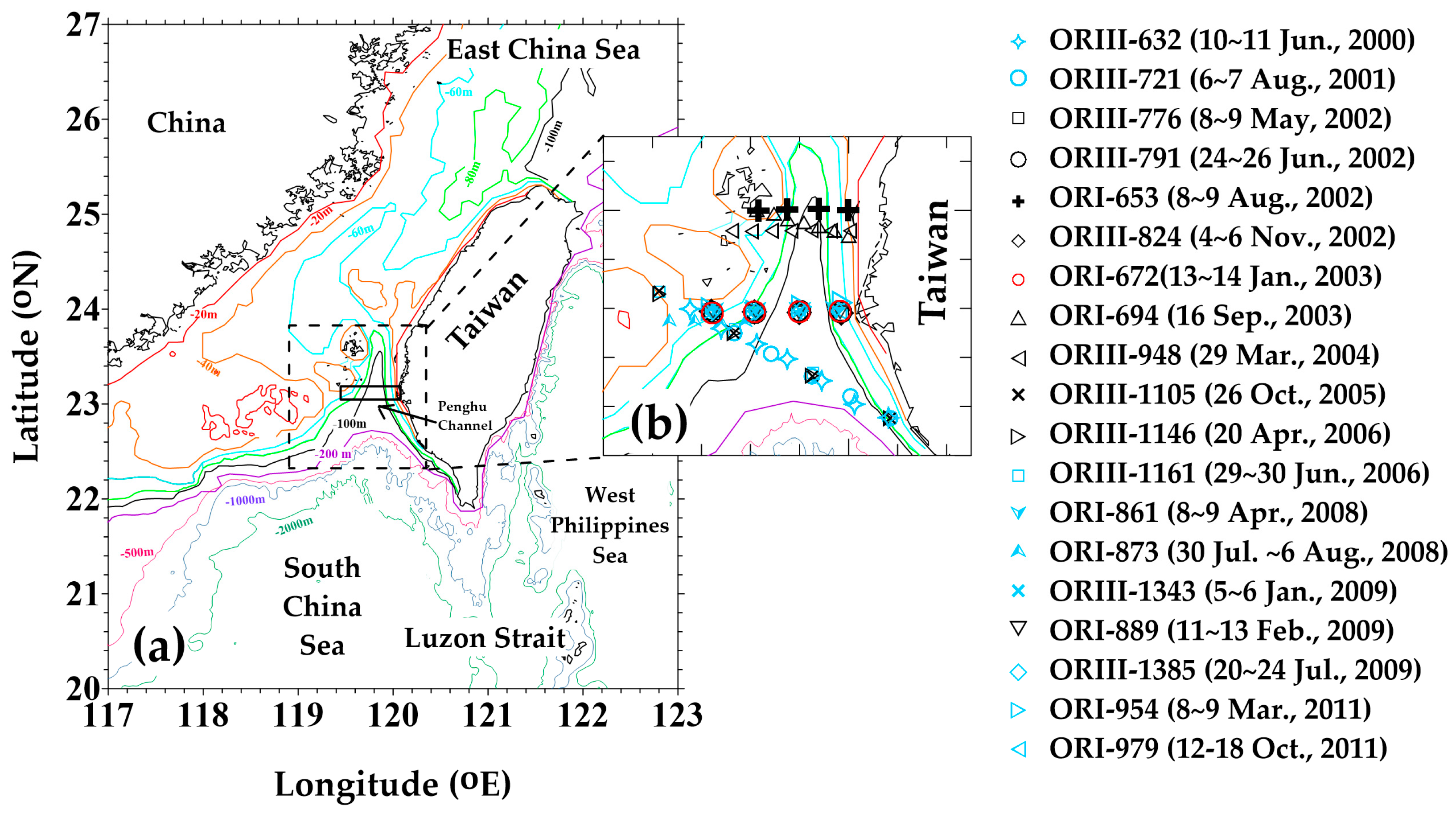
To estimate continuous nutrient and inorganic carbon fluxes, the chemical concentrations were simulated based on the measured data. The daily salinity, temperature, and flow velocity in the PHC were obtained using the Hybrid Coordinate Ocean Model (HYCOM). The sampling sites are located between 22.5–23.5° N and 119.5–120.1° E (Figure 1), and most of them are close to 23° N. A total of 555 bottle samples were collected during 19 cruises from 2000 to 2011 using a CTD/Rosette sampler, while salinity and temperature were recorded in situ. The nutrient concentrations were determined by published methods with flow injection analyzers. Nitrate plus nitrite (N) are the major species of dissolved inorganic nitrogen in the seawater, and the N concentration was obtained using the pink azo dye method [22], with a precision of approximately ±1% at 35 μmol kg−1 and ±3% at 1 μmol kg−1. Phosphate (P) concentration was measured using the molybdenum blue method [23] with a precision of approximately ±0.5% at 2.5 μmol kg−1 and ±3% at 0.1 μmol kg−1. Silicate (Si) concentration was measured using the silicon molybdenum blue method with a precision of around 0.6% at 150 μmol kg−1 and 2% at 5 μmol kg−1. DIC concentration was determined using 10% phosphoric acid to acidify the samples, and then quantifying the produced CO2 gas using an infrared gas analyzer (AS-C3 Apollo Scitech), a single operator multi-parameter metabolic analyzer (SOMMA), or a coulometric detector. TA was measured using the open-cell method of potentiometric titration at 25 °C with a PC-controlled titration cell [24,25]. The end points of titration were determined using the Gran Function with a precision of 0.1% [26].
To estimate the daily average chemical concentrations, simulation models were derived using in situ temperature, salinity, and measured chemical concentrations. A second-order polynomial regression model was selected using leave-one-out cross-validation because it minimized the mean square error of prediction [27]. (See Appendix A for more detail.) Table 1 presents the coefficients of regression fits, residual standard error, and adjusted coefficients of determination. Each adjusted determination coefficient between the seasonal chemical simulation result and the measured data exceeded 0.7, so the model captured more than 70% of the variability of the original data. The low probability values (p < 0.001) suggest that simulation models are compatible with the measured data (Table 1). To compare the measured and fitted results, the mentioned equations (Table 1) and the in situ temperature and salinity values that were collected with bottle samples were utilized to calculate the fitted chemical concentrations. Significant positive correlations existed between the approximately 500 measured and fitted values of TA, DIC, N, P, and Si concentrations, and the simulated performance values expressed more than 88% of measured data, according to the determination coefficients (Figure 2).
To quantify the contribution from each predictor variable to simulation results, the R-squared values in different situations were calculated. The temperature is more important than the salinity as a predictor variable in the chemical concentration models except for TA fitted model during winter and spring (Table 2). Comparing in situ temperature and the daily temperature that was simulated using the HYCOM demonstrates that the simulation yielded underestimates in the surface layer (0–55 m) but overestimates in the bottom layer (55–125 m, Figure 3a). On the contrary, the HYCOM salinity and fitted N values were overestimated in the surface layer but were underestimated in the bottom (Figure 3b,c). Since temperature is the major controlling factor in the chemical model, the differences between the in situ temperature and the HYCOM model temperature caused simulated N concentrations to vary. There were larger variations in the bottom layers of temperature and N differences than in the surface layers, but the variation of salinity difference was lower in the bottom layer than in the surface layer (Figure 3). The results also support the conclusion that the simulated N concentrations are less influenced by salinity than by temperature. The differences between simulated and measured data may have had the following few causes; (1) the variation between each single measurement and the daily average; (2) the assumption that biological production and consumption do not vary within a season; (3) the simplification of chemical concentrations using a fixed water mass mixing ratio between the SCS and WPS waters; and (4) the deviation of HYCOM results.
To estimate the daily average concentration of each chemical parameter, the double integral mean value theorem was used. By Chebyshev’s inequality [28], the true values of daily salinity () and temperature () are 75% likely to be within two deviations of the daily average of salinity () and two deviations of the daily average temperature () if and are close to the true standard deviations. Let be the mean value of over the above intervals under the model. According to the mean value theorem for a double integral [29],
With properly defined and , can be regarded as an approximation to the true daily average of a chemical parameter in the model. Appendix A presents details of the model selection and the fitted daily average values of chemical parameters.
The daily salinity, temperature, and water velocity along 23.04° N from 119.44 to 120.08° E were obtained using HYCOM + NCODA (Navy Coupled Ocean Data Assimilation) Global 1/12° Reanalysis from January 1993 to December 2012. Water flux was calculated using the daily model water velocity (v; m s−1), the depth layer (diz; m), and the distance between two adjacent stations (dx; m):
where i and n are the index of a station and the total number of stations, respectively; k is the layer number at the ith station; ki is the bottom layer at the ith station. The chemical fluxes were generated as:
where C(x, z) was calculated from the aforementioned second-order polynomial regression models and the double integral mean value. The unit of the chemical fluxestimated at the study section is mole s−1. The positive value represents a northward transport chemical quantity through the profile, and negative value is a southward transport.
3. Results
3.1. Seasonal Profiles
Since the PHC is directly and indirectly influenced by seasonal monsoons, the seawater mixing ratio and water transport velocity vary over time. The model salinity increased with depth from 33.9 to 34.8, but the temperature decreased with depth from 29 °C to 18 °C (Figure 4a–d). The salinity and temperature in winter and spring varied little between the surface and bottom layers, whereas those in summer and autumn varied more (Figure 4a,b). The differences in salinity and temperature between the surface and bottom layers were largest in the summer, and the highest and lowest salinities and temperatures were also found in this season (Figure 4c,d). The distribution of the P concentration followed the salinity distribution, and the P concentration is the highest in the bottom layer in summer. However, the distribution of the velocity differs from those of the aforementioned parameters. In autumn and winter, the velocity is highest in the middle layer of the deepest part of the PHC around 119.8° E (Figure 4e,h), but in spring and summer, it is highest in the surface layer (Figure 4f,g).
3.2. Time Series of Estimated Fluxes and Physical Data
The simulated physical data and fluxes exhibit obvious seasonal variations (Figure 5). The 20-year average water velocity (1993–2012) is around 0.15 ± 0.08 m s−1 northward, but the velocities become negative values southward during the La Niña winters (January, December 2011 and January 2012; grey areas in Figure 5a). The average water flux is 0.81 ± 0.43 Sverdrup (Sv, 1 Sv = 106 m3 s−1), which is approximately 41~68% of the reported water transport in the TS (1.2~2.0 Sv) [30,31,32]. The annual average TA, DIC, N, P, and Si fluxes are 1.87 ± 0.79 × 10⁶ mol C s−1, 1.65 ± 0.71 × 10⁶ mol C s−1, 1203 ± 994 mol N s−1, 132 ± 85 mol P s−1, and 3062 ± 1828 mol Si s−1, respectively. The area of study section is 5.4 km2, and the average TA, DIC, N, P, and Si per-area fluxes are 346 kmol C km−2 s−1, 306 kmol C km−2 s−1, 0.2 kmol N km−2 s−1, 0.02 kmol P km−2 s−1, and 0.6 kmol Si km−2 s−1.
The PHC is divided into top and bottom layers (red and blue lines in Figure 5) at depths of 0–55 m and 55–125 m, respectively. The cross-sectional areas of the top and bottom layers are 3.5 km2 and 1.9 km2, respectively. The average velocity, water flux, area-weighted temperature, TA, and DIC fluxes in the top layer exceed those in the bottom layer. On the other hand, the area-weighted salinity and nutrient fluxes in the bottom layer exceed those in the top layer. The annual average TA, DIC, N, P, and Si fluxes in the top layer (bottom layer) are, 1.39(0.48) × 106 mol C s−1, 1.20(0.45) × 106 mol C s−1, 517(686) mol N s−1, 71(61) mol P s−1, and 1800(1262) mol Si s−1, respectively.
3.3. Comparison between Measured and Simulated Data
To compare the data measured in situ in 19 cruises with the simulated data, the weighted-average gridding method in Ocean Data View [33] was used to interpolate and extrapolate data associated with a single profile along 23.04° N from 119.4 to 120.08° E. The average differences (simulated—measured in 19 cruises) in salinity (ΔS) and temperature (ΔT) are 0.063 ± 0.237 and 0.246 ± 1.086 °C, respectively. For TA, DIC, N, P, and Si fluxes, the average differences are 0.001 ± 0.017 × 10⁶ mol C s−1 (ΔTA), −0.010 ± 0.033 × 10⁶ mol C s−1 (ΔDIC), −409 ± 1064 mol N s−1 (ΔN), −22 ± 68 mol P s−1 (ΔP), and −588 ± 1664 mol Si s−1 (ΔSi), respectively. Generally, the simulated data yield overestimates of salinity, temperature, and TA flux, but underestimates of DIC, N, P, and Si fluxes. The ΔTA and ΔDIC fluxes positively correlate with ΔS, but the differences ΔN, ΔP, and ΔSi fluxes are negatively correlated with ΔT (Figure 6). The daily chemical concentration was calculated by averaging the maxima and minima of the estimated concentrations that were mentioned in Section 2.
4. Discussion
4.1. Annual Variation
The two major factors that drive water transportation in the TS are wind stress and a northward pressure gradient force that arises from the fact that the surface of the south TS is higher than that of the north TS. Southwest monsoons accelerate northward flow during the summer, but northeast monsoons reduce it, even reversing it to southward flow during the period of strong northeasterly winds [10,15,34,35].
The monthly values of fluxes and parameters exhibit four patterns. First, the water, TA, and DIC fluxes (Figure 7a,d,e) are highest in July. The TA and DIC fluxes basically reflect the variation of water flux, since the seasonal percentage differences of TA and DIC concentrations are smaller than the variations of the nutrient concentrations (Figure 7). Second, the salinity, TA, and DIC concentrations are lowest in September (Figure 7b,d,e). The third pattern contrasts with the second, as the temperature is highest in September (Figure 7c). During the summer and autumn, the main water mass in the PHC is the SCS water, which has a lower salinity than the WPS water at the same density in surface water. Since precipitation in the summer is heavy, the water in the top layer is warmer and fresher during the summer than the autumn. Yet, the strong summer water flow carries the colder and saltier deeper water into the PHC (Figure 4b,f). The northward current is weakened in autumn owing to the onset of the northeast monsoon, and reduces the coldness and saltiness of the seawater in the bottom. The area-weighted salinity is lowest in September, when the area-weighted temperature is highest. This phenomenon is consistent with the significant influence of the salty bottom water in the summer. Fourth, the N, P, and Si fluxes are highest in June (Figure 7f,g,h). The high water flux increases nutrient fluxes in the summer as the deeper water contains higher nutrient concentrations.
4.2. Interannual Variations
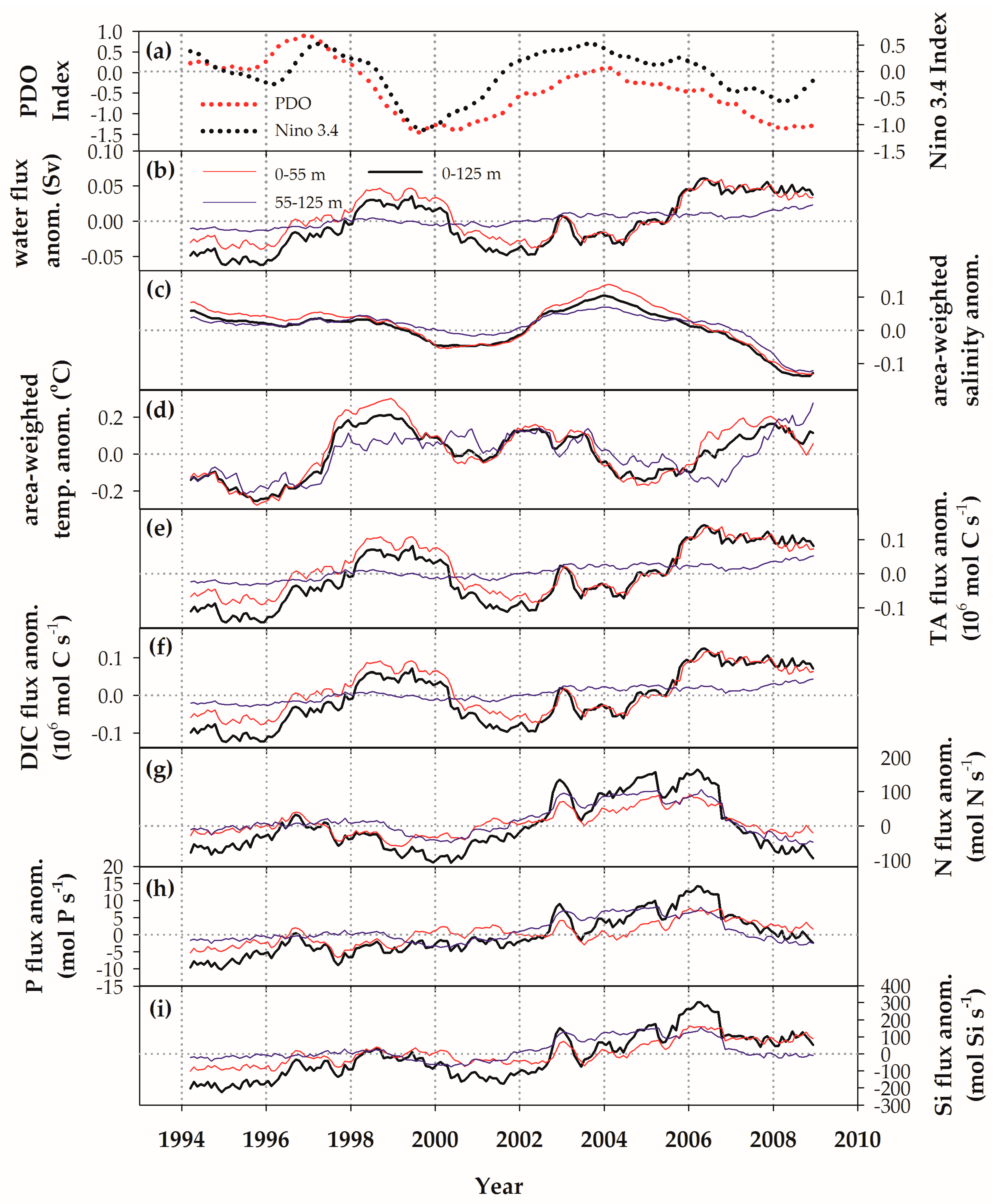
To determine simplified patterns of the anomalous flux of TA, DIC, N, P, and Si, 30-month moving averages were used to eliminate any seasonal pattern (Figure 8). Since the unusual negative water fluxes in January 2011, January and December 2012 substantially influence the averaged values, only data from January 1993 to December 2010 were considered. The 30-month moving average patterns of PDO and El Niño 3.4 index are similar, with two obvious maxima in 1997 and 2004, and minima in 2000 and 2008, respectively (Figure 8a). The two anomalous two-year maxima of the water, TA, and DIC fluxes were in 1998–2000 and 2006–2008, respectively; and the two minima were in 1994–1996 and roughly 2002–2004 (Figure 8b,e,f; 0–55 m, 0–125 m). One obvious anomalous salinity maximum occurred in 2004, and two anomalous salinity minima occurred in 2001 and 2009 (Figure 8c). The pattern of temperature anomalies is complex. Three maxima around 1999, 2002–2003, and 2008, and three minima in 1996, 2001, and 2005 are observed (Figure 8d). With respect to anomalous nutrient fluxes, one obvious maximum in 2004–2007 and one fuzzy maximum in 1996–1998 are observed. One obvious minimum of nutrients fluxes occurs in 2008, and one fuzzy minimum occurs in 1999 (Figure 8g–i).
Generally, the variation of the 30-month moving average PDO index tends to oppose that of water volume in the top layer, but the values in both layers increase slightly with time (Figure 8b). For the top layer, the increased PDO index is related to the reduced water flux and vice versa. The anomalous salinity patterns in both layers mirror the pattern of the PDO index, and decrease slightly over time (Figure 8b). The salinity abatement may be an indirect effect of the reduced Kuroshio intrusion, and a simulated low salinity in 2001 has been reported [36]. If the decreased salinity is caused by the reduced Kuroshio intrusion, then the temperature will decrease with the low salinity event in 2001. However, the low salinity event in 2008 is associated with a high temperature signal, suggesting that Kuroshio intrusion may not be the only factor that controls water mass mixing in the PHC (Figure 8c,d). The anomalous TA and DIC patterns are similar to the anomalous water flux, and also increase with time (Figure 8e,f). Generally, the TA and DIC fluxes rise as the PDO index decreases. However, the nutrient fluxes vary with the PDO index, indicating that the nutrient concentrations are the main controlling factor. The anomalous nutrient fluxes also increase slightly with time (Figure 8g–i).
5. Conclusions
The simulated chemical fluxes of TA, DIC, N, P, and Si are calculated from estimated chemical concentrations using individual second-order polynomial regression equations and water flux that is obtained using the HYCOM. Equations for TA, DIC, N, P, and Si concentrations were derived using chemical concentrations that were measured from bottle samples, in situ salinity, and temperature. All the chemical models presented herein explained more than 70% of the variability of the original data. The individual daily chemical concentrations in various locations and at different water depths were calculated using the derived equations and the daily salinity and temperature values that were obtained using the HYCOM. The error ranges of the simulated chemical concentrations were estimated using the double integral mean value theorem. The estimated annual northward fluxes of TA, DIC, N, P, and Si are, 1.87 ± 0.79 × 10⁶ mol C s−1, 1.65 ± 0.71 × 10⁶ mol C s−1, 1203 ± 994 mol N s−1, 132 ± 85 mol P s−1, and 3062 ± 1828 mol Si s−1, respectively. The TA, DIC, P, and Si are transported principally in the top layer, but the N flux is mainly transported in the bottom layer. The high water flux in the summer is mostly responsible for the highest chemical fluxes in the whole year. There are two kinds of chemical flux patterns. For the anomalous 30-month moving average TA and DIC, the patterns follow that of the water flux. On the contrary, the patterns of anomalous 30-month moving average nutrient fluxes are oppose to that of the water flux, but follow that of the PDO index. The largest increases of N, P, and Si fluxes are around 10 to 20% in the period of rising PDO index, especially during 2004–2007.
Acknowledgments
We thank the anonymous reviewers for their insightful comments and suggestions improving this article. The Ministry of Science and Technology of Taiwan, provided financial assistance for this work (MOST 106-2611-M-110-016 and 106-2811-M-110-019). The authors thank Aycil Cesmelioglu, Anna Spagnuolo, and Ravindra Khattree from the Department of Mathematics and Statistics at Oakland University, who offered valuable comments on the numerical and statistical analysis.
Author Contributions
C.-T.A.C. and T.-H.H. conceived and designed the experiments; T.-H.H. and Z.L. analyzed the data; C.-R.W. contributed data interpretation; T.-H.H., C.-T.A.C., and Z.L. wrote the paper.
Conflicts of Interest
The authors declare no conflicts of interest.
Appendix A
Appendix A.1. Model Selection
Model selection was based upon the analysis of the mean square error (MSE) of prediction using leave-one-out cross-validation [27], which estimates the prediction performance for the first, second, and third order polynomial regression model, respectively. The smaller MSE of prediction indicates the regression model has better performance in prediction. Using leave-one-out cross-validation, the set of observations was repeatedly split into a validation set containing a single observation and a training set containing the remaining observations. By repeating the prediction of the validation set using the model fitted by the training set, MSE was obtained by computing the average of summation of squared residuals, which are the differences between observed and predicted values for each order polynomial function. The second-order polynomial regression model with interaction term was found with the smallest MSE of prediction on all chemical parameters and hence was chosen for fitting TA, DIC, N, P and Si, respectively.
Appendix A.2. Prediction Interval of Daily Average of Chemical Parameters
In this section, we use an approach to estimate the prediction interval of the daily average for each chemical parameter by using the mean value of function for double integrals, although the probability density functions of daily salinity and temperature are unknown. Let and be the assimilated daily average of salinity and temperature from HYCOM, respectively. Also, let and be the deviations from the mean of daily salinity and temperature, and be the fitted second-order polynomial regression function with respect to salinity and temperature . We assume that and approximate to the true mean of distribution of daily salinity and temperature, respectively. By Chebyshev’s inequality [28], there is at least a 75% chance that the true values of daily salinity and temperature fall within the interval of salinity and temperature if and are close to the true standard deviations. Let be the mean value of over the above intervals under the model. According to the mean value theorem for double integrals [29], we have
With properly chosen and , can be viewed as an approximation of the true daily average of a chemical parameter under the model. Choosing larger and will mean take irrelevant data into account, while choosing smaller and will mean ignores true values outside of the region. Instead of finding the optimal and , we seek the interval that more likely bounds the true daily average of chemical parameter under the model because we have no information about the distribution of daily salinity and temperature. Based on the observed standard deviation from measured salinity data among four seasons—0.25 (Winter), 0.22 (Spring), 0.76 (Summer), and 0.39 (Autumn), we fix the . for each season as 0.25 (Winter), 0.25 (Spring), 0.75 (Summer), and 0.50 (Autumn) because we assume that the daily standard deviation is small and is at most equal to the seasonal standard deviation. We choose different from small to large in order to obtain the prediction interval of since we consider temperature to have a more significant effect than salinity does on chemical parameters. Based on the statistics from Dongjidao Wave Station of the Center Weather Bureau, all the choices of are 1 °C and 2 °C for spring, summer, and autumn, as the observed standard deviation is 2 °C. And is 1 °C for winter, as the observed standard deviation is 1 °C. As the quantity is the lower or upper bound of when is convex or concave over some specific region, we still include to determine the endpoint of the prediction interval. Let and be the minimum and maximum value among the set containing those ’s computed by different choices of and . Therefore, is the prediction interval of the daily average for the chemical parameter, given and .
References
- Chen, C.T.A.; Jan, S.; Huang, T.H.; Tseng, Y.H. Spring of no Kuroshio intrusion in the southern Taiwan Strait. J. Geophys. Res. Oceans 2010, 115, C08011. [Google Scholar] [CrossRef]
- Han, A.; Dai, M.; Gan, J.; Kao, S.-J.; Zhao, X.; Jan, S.; Li, Q.; Lin, H.; Chen, C.-T.; Wang, L. Inter-shelf nutrient transport from the East China Sea as a major nutrient source supporting winter primary production on the northeast South China Sea shelf. Biogeosciences 2013, 10, 8159–8170. [Google Scholar] [CrossRef]
- Chen, C.T.A.; Wang, S.L. Carbon, alkalinity and nutrient budgets on the East China Sea continental shelf. J. Geophys. Res. Oceans 1999, 104, 20675–20686. [Google Scholar] [CrossRef]
- Chen, C. The Kuroshio Intermediate Water is the major source of nutrients on the East China Sea continental shelf. Oceanol. Acta 1996, 19, 523–527. [Google Scholar]
- Li, M.; Xu, K.; Watanabe, M.; Chen, Z. Long-term variations in dissolved silicate, nitrogen, and phosphorus flux from the Yangtze River into the East China Sea and impacts on estuarine ecosystem. Estuar. Coast. Shelf Sci. 2007, 71, 3–12. [Google Scholar] [CrossRef]
- Zhou, M.-J.; Shen, Z.-L.; Yu, R.-C. Responses of a coastal phytoplankton community to increased nutrient input from the Changjiang (Yangtze) River. Cont. Shelf Res. 2008, 28, 1483–1489. [Google Scholar] [CrossRef]
- Gong, G.C.; Chang, J.; Chiang, K.P.; Hsiung, T.M.; Hung, C.C.; Duan, S.W.; Codispoti, L. Reduction of primary production and changing of nutrient ratio in the East China Sea: Effect of the three gorges dam? Geophys. Res. Lett. 2006, 33, L07610. [Google Scholar] [CrossRef]
- Lee, K.; Matsuno, T.; Endoh, T.; Ishizaka, J.; Zhu, Y.; Takeda, S.; Sukigara, C. A role of vertical mixing on nutrient supply into the subsurface chlorophyll maximum in the shelf region of the East China Sea. Cont. Shelf Res. 2017, 143, 139–150. [Google Scholar] [CrossRef]
- Liu, K.-K.; Tang, T.Y.; Gong, G.-C.; Chen, L.-Y.; Shiah, F.-K. Cross-shelf and along-shelf nutrient fluxes derived from flow fields and chemical hydrography observed in the southern East China Sea off northern Taiwan. Cont. Shelf Res. 2000, 20, 493–523. [Google Scholar] [CrossRef]
- Chen, C.-T.A. Rare northward flow in the Taiwan Strait in winter: A note. Cont. Shelf Res. 2003, 23, 387–391. [Google Scholar] [CrossRef]
- Chung, S.-W.; Jan, S.; Liu, K.-K. Nutrient fluxes through the Taiwan Strait in spring and summer 1999. J. Oceanogr. 2001, 57, 47–53. [Google Scholar] [CrossRef]
- Jan, S.; Sheu, D.D.; Kuo, H.M. Water mass and throughflow transport variability in the Taiwan Strait. J. Geophys. Res. Oceans 2006, 111, C12012. [Google Scholar] [CrossRef]
- Lin, S.; Tang, T.; Jan, S.; Chen, C.-J. Taiwan Strait current in winter. Cont. Shelf Res. 2005, 25, 1023–1042. [Google Scholar] [CrossRef]
- Naik, H.; Chen, C.-T.A. Biogeochemical cycling in the Taiwan Strait. Estuar. Coast. Shelf Sci. 2008, 78, 603–612. [Google Scholar] [CrossRef]
- Wu, C.-R.; Chao, S.-Y.; Hsu, C. Transient, seasonal and interannual variability of the Taiwan Strait current. J. Oceanogr. 2007, 63, 821–833. [Google Scholar] [CrossRef]
- Zhang, W.-Z.; Chai, F.; Hong, H.-S.; Xue, H. Volume transport through the Taiwan Strait and the effect of synoptic events. Cont. Shelf Res. 2014, 88, 117–125. [Google Scholar] [CrossRef]
- Huang, T.-H.; Chen, C.-T.A.; Zhang, W.-Z.; Zhuang, X.-F. Varying intensity of Kuroshio intrusion into southeast Taiwan Strait during ENSO events. Cont. Shelf Res. 2015, 103, 79–87. [Google Scholar] [CrossRef]
- Qu, T.; Mitsudera, H.; Yamagata, T. Intrusion of the north Pacific waters into the South China Sea. J. Geophys. Res. Oceans 2000, 105, 6415–6424. [Google Scholar] [CrossRef]
- Qu, T.; Kim, Y.Y.; Yaremchuk, M.; Tozuka, T.; Ishida, A.; Yamagata, T. Can Luzon Strait transport play a role in conveying the impact of ENSO to the South China Sea? J. Clim. 2004, 17, 3644–3657. [Google Scholar] [CrossRef]
- Wu, C.-R.; Wang, Y.-L.; Lin, Y.-F.; Chao, S.-Y. Intrusion of the Kuroshio into the South and East China Seas. Sci. Rep. 2017, 7, 7895. [Google Scholar] [CrossRef] [PubMed]
- Gong, G.-C.; Liu, K.K.; Liu, C.-T.; Pai, S.-C. The chemical hydrography of the South China Sea west of Luzon and a comparison with the West Philippine Sea. Terr. Atmos. Ocean Sci. 1992, 3, 587–602. [Google Scholar] [CrossRef]
- Pai, S.-C.; Yang, C.-C.; Riley, J.P. Formation kinetics of the pink azo dye in the determination of nitrite in natural waters. Anal. Chim. Acta 1990, 232, 345–349. [Google Scholar] [CrossRef]
- Pai, S.-C.; Yang, C.-C.; Riley, J. Effects of acidity and molybdate concentration on the kinetics of the formation of the phosphoantimonylmolybdenum blue complex. Anal. Chim. Acta 1990, 229, 115–120. [Google Scholar] [CrossRef]
- Cai, W.J.; Hu, X.; Huang, W.J.; Jiang, L.Q.; Wang, Y.; Peng, T.H.; Zhang, X. Alkalinity distribution in the western North Atlantic Ocean margins. J. Geophys. Res. Oceans 2010, 115, C08014. [Google Scholar] [CrossRef]
- Chen, C.; Wang, S. International intercalibration of carbonate parameters. Acta Oceanol. Sin. 1993, 15, 60–67. [Google Scholar]
- Gran, G. Determination of the equivalence point in potentiometric titrations. Part II. Analyst 1952, 77, 661–671. [Google Scholar] [CrossRef]
- James, G.; Witten, D.; Hastie, T.; Tibshirani, R. An Introduction to Statistical Learning: With Applications in R; Springer: New York, NY, USA, 2013; ISBN 978-1-4614-7138-7. [Google Scholar]
- Casella, G.; Berger, R.L. Statistical Inference; Brooks-Cole: Pacific Grove, CA, USA, 2002; ISBN 978-0-5342-4312-8. [Google Scholar]
- Buck, R.C. Advanced Calculus; Waveland Press: Long Grove, IL, USA, 1978; ISBN 978-0-0700-8728-6. [Google Scholar]
- Isobe, A. Recent advances in ocean-circulation research on the Yellow Sea and East China Sea shelves. J. Oceanogr. 2008, 64, 569–584. [Google Scholar] [CrossRef]
- Fang, G.; Zhao, B.; Zhu, Y. Water volume transport through the Taiwan Strait and the continental shelf of the East China Sea measured with current meters. Elsevier Oceanogr. Ser. 1991, 54, 345–358. [Google Scholar] [CrossRef]
- Wang, Y.; Jan, S.; Wang, D. Transports and tidal current estimates in the Taiwan Strait from shipboard ADCP observations (1999–2001). Estuar. Coast. Shelf Sci. 2003, 57, 193–199. [Google Scholar] [CrossRef]
- Schlitzer, R. Ocean Data View. 2016. Available online: https://odv.awi.de/ (accessed on 31 December 2017).
- Jan, S.; Chao, S.-Y. Seasonal variation of volume transport in the major inflow region of the Taiwan Strait: The Penghu Channel. Deep Sea Res. Part II 2003, 50, 1117–1126. [Google Scholar] [CrossRef]
- Wu, C.R.; Chang, C.W. Interannual variability of the South China Sea in a data assimilation model. Geophys. Res. Lett. 2005, 32, L17611. [Google Scholar] [CrossRef]
- Nan, F.; Yu, F.; Xue, H.; Zeng, L.; Wang, D.; Yang, S.; Nguyen, K.-C. Freshening of the upper ocean in the South China Sea since the early 1990s. Deep Sea Res. Part I 2016, 118, 20–29. [Google Scholar] [CrossRef]
Figure 1.
Sampling area. (a) Black square delineates HYCOM data area; and (b) symbols represent stations where water is sampled.
Figure 1.
Sampling area. (a) Black square delineates HYCOM data area; and (b) symbols represent stations where water is sampled.

Figure 2.
The correlations between fitted and measured concentrations of (a) TA; (b) DIC; (c) N; (d) P; and (e) Si. The fitted data were calculated based on the equations for four seasons in Table 1 at the temperature and salinity of bottle samples.
Figure 2.
The correlations between fitted and measured concentrations of (a) TA; (b) DIC; (c) N; (d) P; and (e) Si. The fitted data were calculated based on the equations for four seasons in Table 1 at the temperature and salinity of bottle samples.
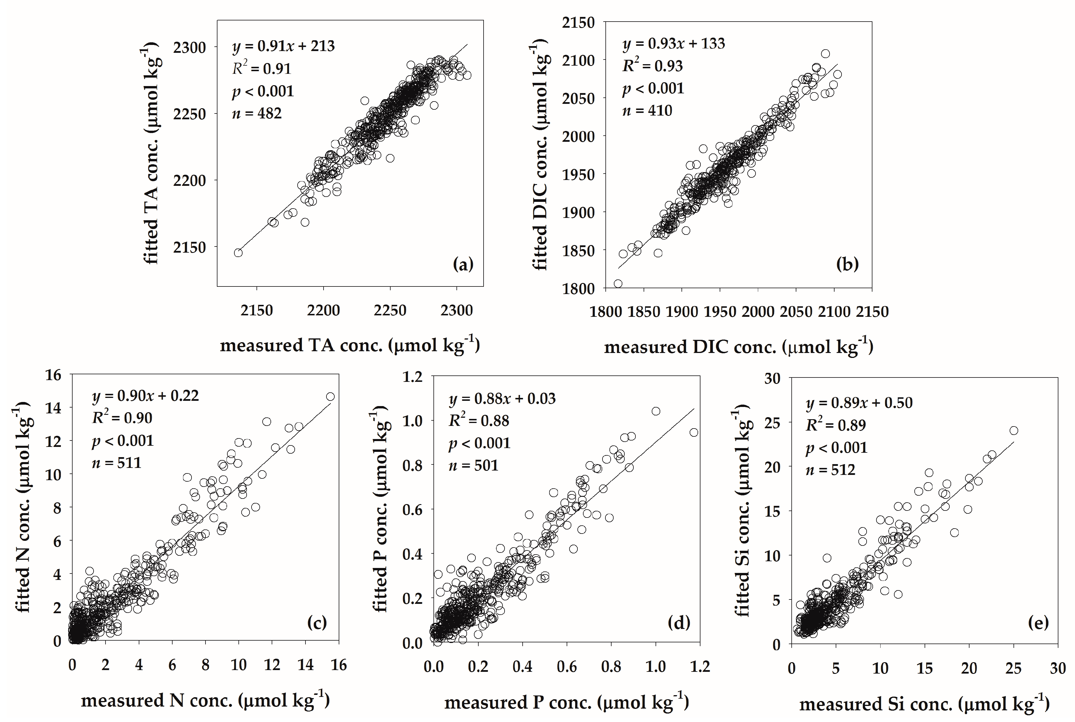
Figure 3.
The correlations between (a) the difference between HYCOM temperature and measured temperature versus measured temperature; (b) the difference between HYCOM salinity and measured salinity versus measured salinity; and (c) the difference between stimulated N concentrations based on HYCOM data and measured N concentration versus measured N concentration.
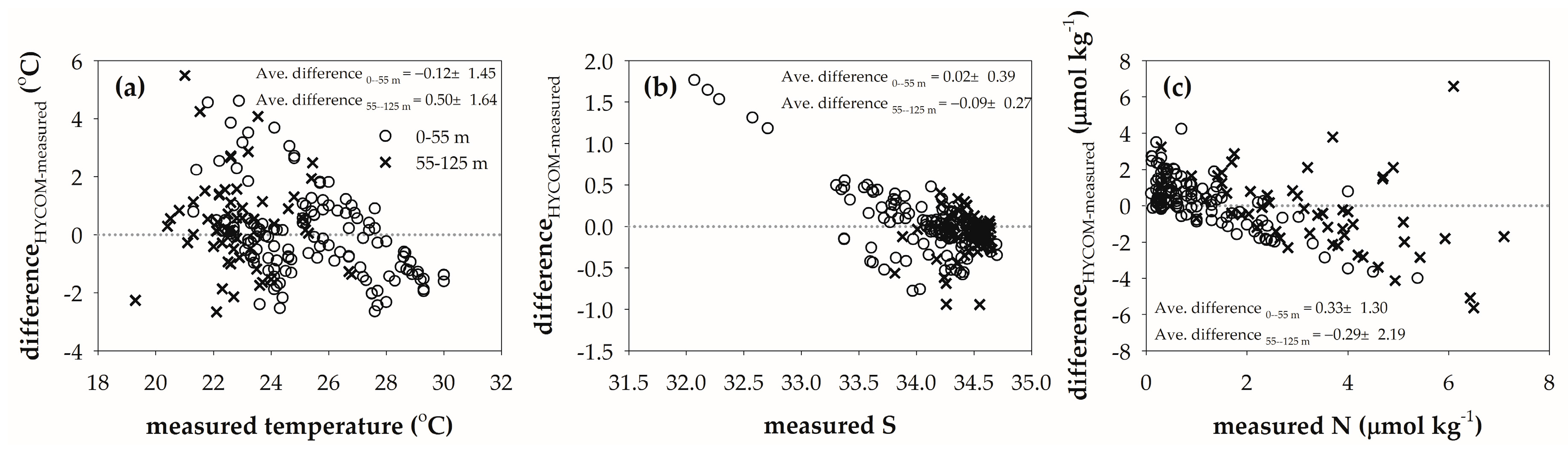
Figure 4.
The left panel is seasonal HYCOM model salinity and temperature profile in the PHC during (a) winter; (b) spring; (c) summer; and (d) autumn. The color area represents different temperature ranges, and the black lines mean salinity contours. The right panel is seasonal HYCOM model velocity and simulated P concentrations in the PHC during (e) winter; (f) spring; (g) summer; and (h) autumn. The color area is different P concentration range, and the positive (negative) values on black lines are northward (southward) velocity.
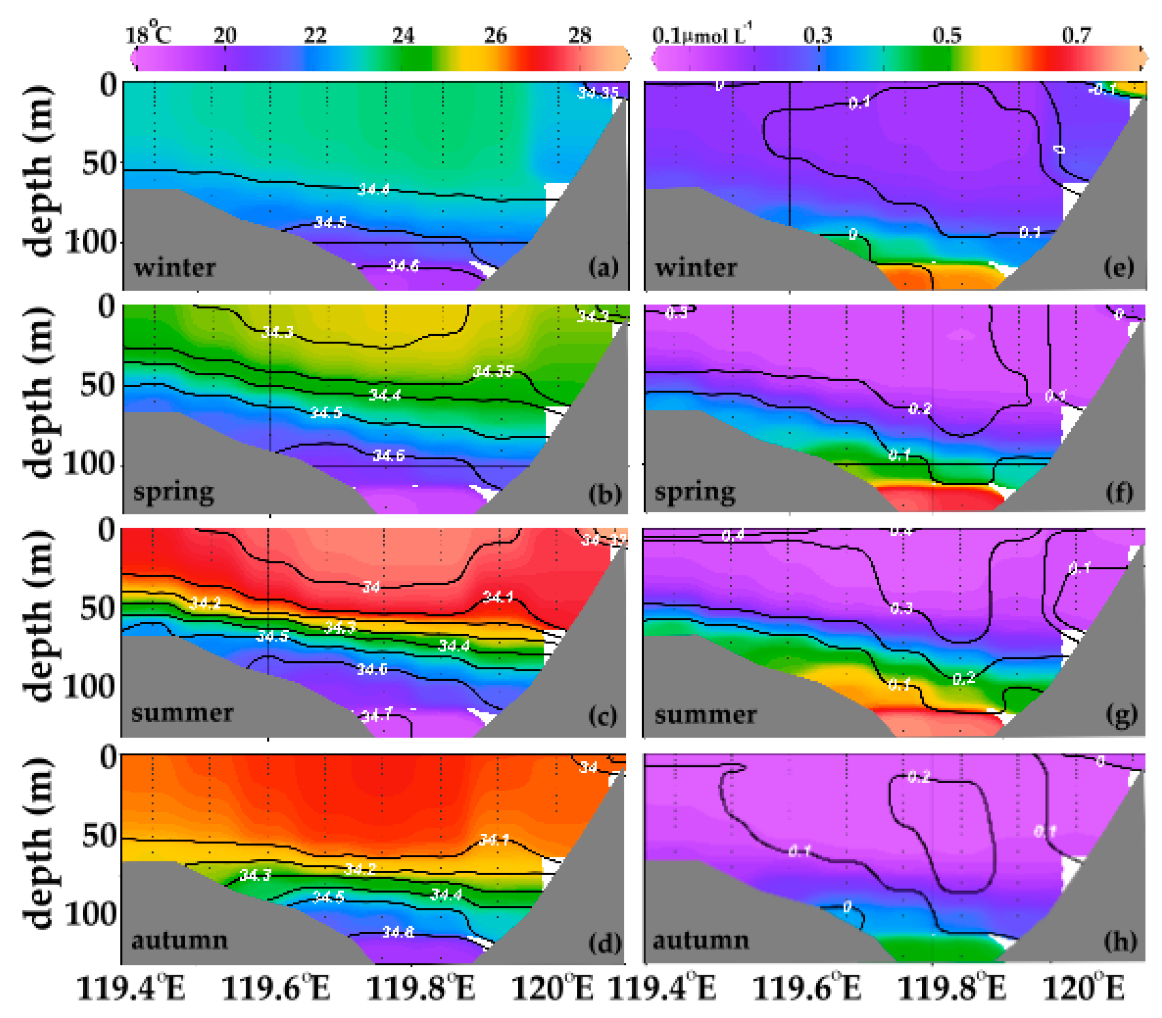
Figure 5.
The time series of (a) water velocity; (b) water flux; (c) area-weighted average salinity; (d) area-weighted average temperature; (e) TA flux, (f) DIC flux; (g) N flux; (h) P flux; and (i) Si flux. The black, red, and blue lines represent the total flux, the top layer (0–55 m) flux, and the bottom layer (55–125 m) flux, respectively. The pink triangles are calculated according to measured chemical concentrations and model water fluxes. The gray shading area denotes the negative (southward) water flux periods.
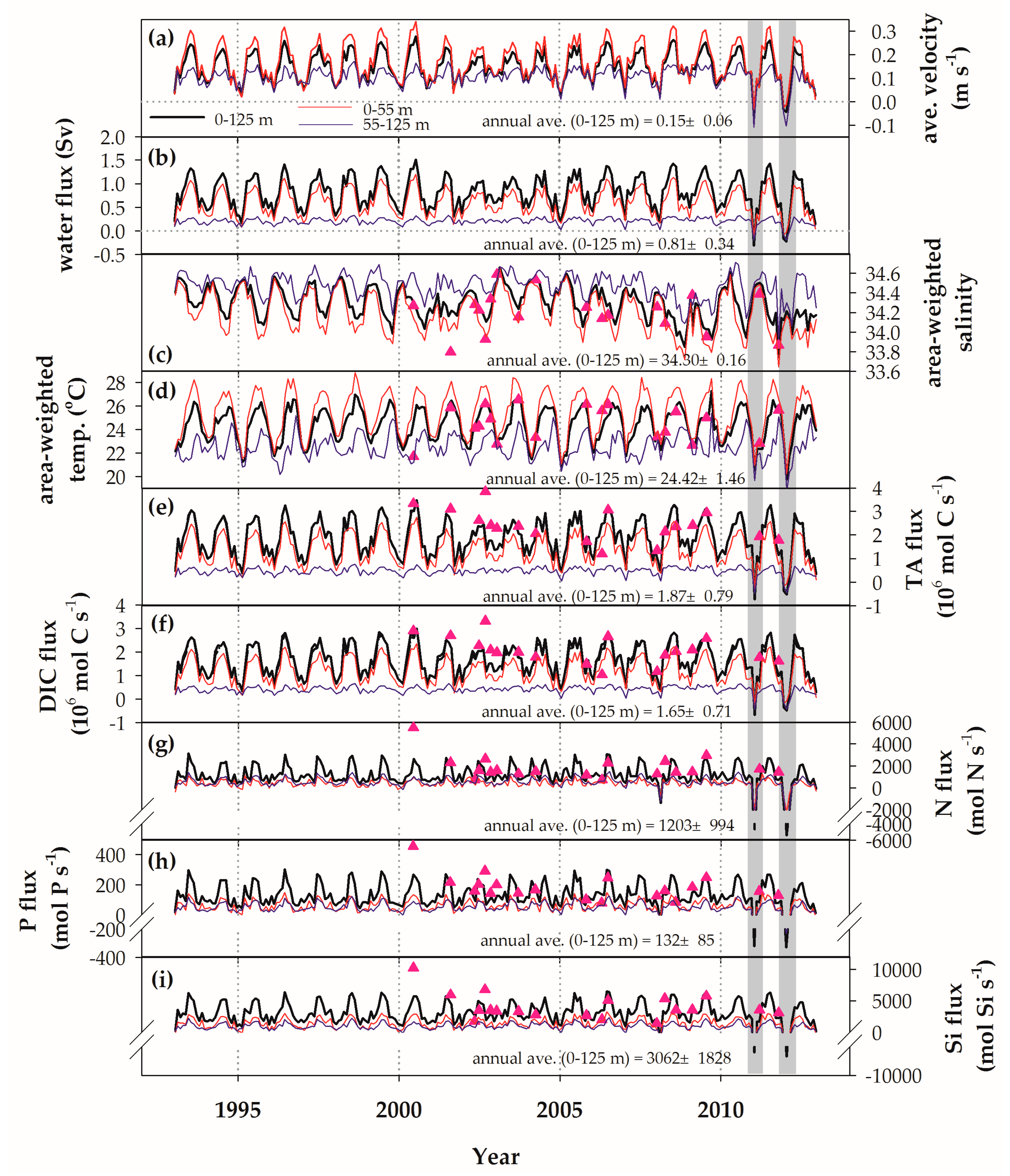
Figure 6.
(a) The differences between simulated fluxes based on TA (DIC) models and measured TA (DIC) concentrations versus the differences of model salinity and in situ salinity; (b) the differences between simulated fluxes based on N (P, Si) models and measured N (P, Si) concentrations versus the differences of model temperature and in situ temperature.
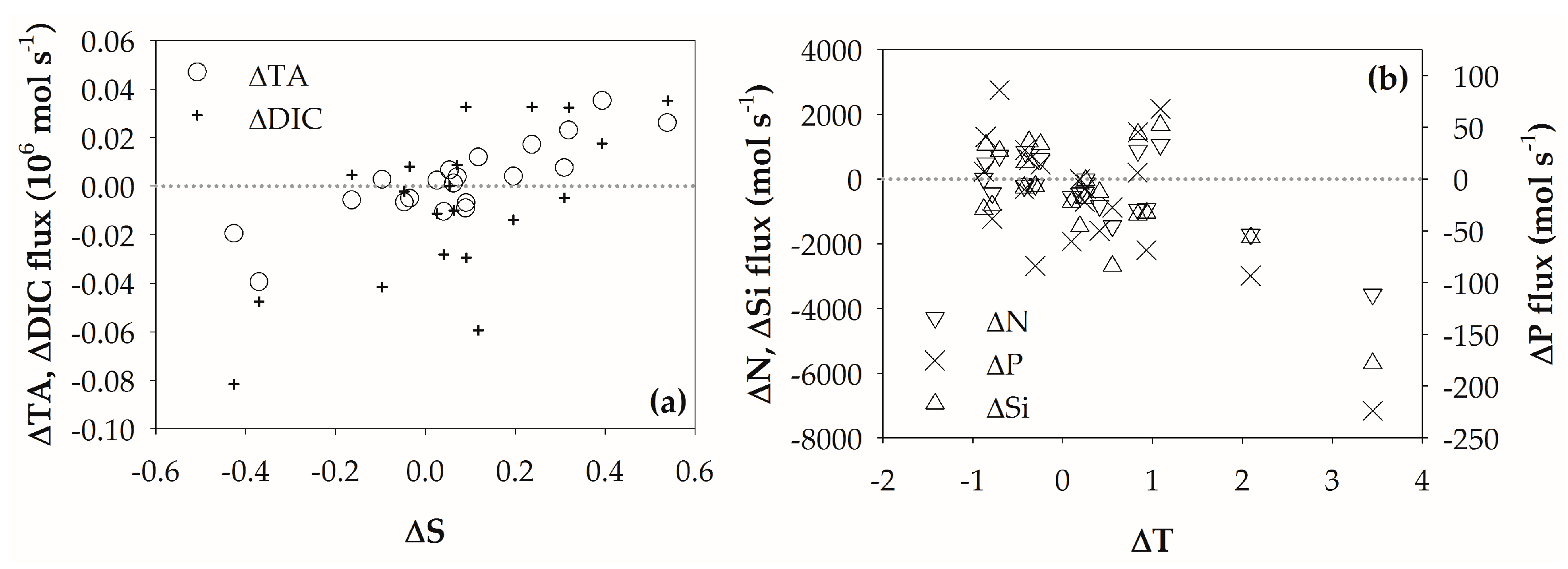
Figure 7.
The monthly average values of (a) water flux; (b) area-weighted salinity; (c) area-weighted temperature; (d) TA concentration and flux; (e) DIC concentration and flux; (f) N concentration and flux; (g) P concentration and flux; and (h) Si concentration and flux. The circles are simulated chemical concentrations, and grey area represents the range between maxima and minima flux.
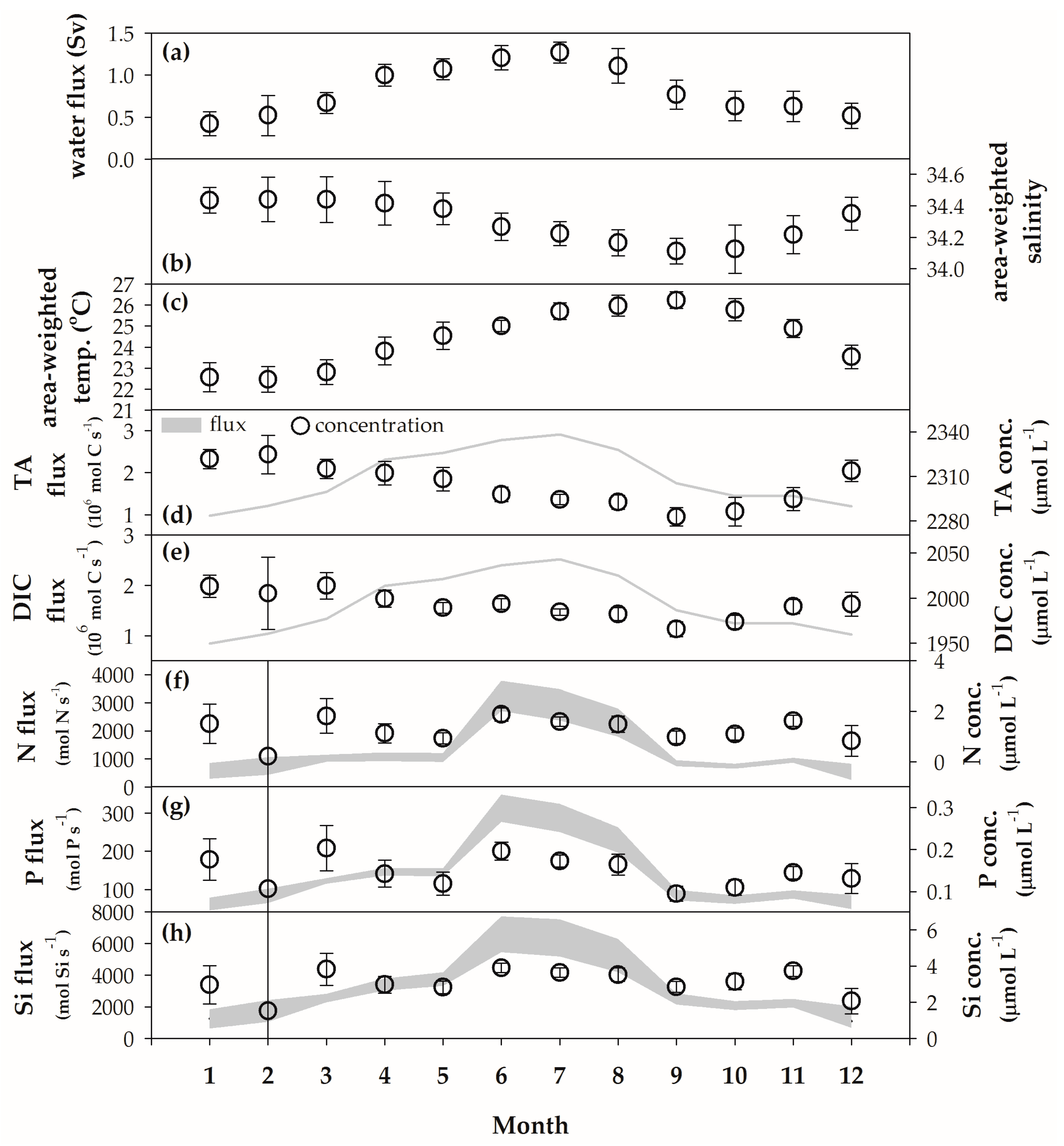
Figure 8.
The 30-month moving average time series of (a) PDO Index and Nino 3.4 Index; (b) water volume anomaly; (c) area-weighted average salinity anomaly; (d) area-weighted average temperature anomaly; (e) TA flux anomaly; (f) DIC flux anomaly; (g) N flux anomaly; (h) P flux anomaly; and (i) Si flux anomaly. The black, red, and blue lines are for the whole section (0–125 m), the mean values in the top layer (0–55 m), and the mean values in the bottom layer (55–125 m).

Table 1.
The constants of seasonal simulated chemical equation, adjusted R-squared (Adj. R2), and residual standard error (RSE) for individual formula.
Table 1.
The constants of seasonal simulated chemical equation, adjusted R-squared (Adj. R2), and residual standard error (RSE) for individual formula.
| Equation | Z = z0 + a × Salinity + b × Temperature + c × Salinity2 + d × Temperature2 + e × Salinity × Temperature | ||||||||
|---|---|---|---|---|---|---|---|---|---|
| Season | Parameter | z0 | a | b | c | d | e | Adj. R2 | RSE |
| winter | TA | −29,747.4 | 1432.897 | 520.565 | −15.022 | −0.890 | −13.908 | 0.83 | 8.0 |
| DIC | −139,348.9 | 7967.724 | 332.260 | −111.891 | 0.000 | −10.115 | 0.88 | 11.0 | |
| N | −3986.3 | 277.336 | −64.615 | −4.549 | 0.264 | 1.487 | 0.87 | 0.9 | |
| P | −221.0 | 14.045 | −1.649 | −0.213 | 0.015 | 0.026 | 0.82 | 0.1 | |
| Si | 5700.9 | −290.119 | −61.750 | 3.811 | 0.364 | 1.264 | 0.82 | 1.4 | |
| spring | TA | 87661.8 | −4651.633 | −529.212 | 63.373 | 0.663 | 14.462 | 0.72 | 6.9 |
| DIC | −98,869.3 | 5492.619 | 528.735 | −73.844 | 0.706 | −16.754 | 0.89 | 9.3 | |
| N | −7366.1 | 406.321 | 33.510 | −5.524 | 0.095 | −1.129 | 0.75 | 0.9 | |
| P | −322.4 | 16.496 | 3.403 | −0.203 | 0.005 | −0.108 | 0.70 | 0.1 | |
| Si | −3730.6 | 200.360 | 26.152 | −2.561 | 0.183 | −1.044 | 0.75 | 1.3 | |
| summer | TA | 10,896.0 | −465.743 | −106.446 | 6.380 | 0.226 | 2.735 | 0.87 | 11.2 |
| DIC | −3359.4 | 287.013 | 0.236 | −3.389 | 0.419 | −0.938 | 0.91 | 19.8 | |
| N | −261.8 | 9.595 | 6.794 | −0.006 | 0.066 | −0.314 | 0.93 | 1.0 | |
| P | -8.9 | 0.126 | 0.423 | 0.007 | 0.004 | −0.019 | 0.94 | 0.1 | |
| Si | 93.8 | 1.514 | −8.143 | −0.026 | 0.141 | 0.004 | 0.92 | 1.5 | |
| autumn | TA | 24,586.7 | −1270.450 | −119.310 | 18.098 | 0.013 | 3.409 | 0.93 | 6.3 |
| DIC | 8352.6 | −433.966 | 48.191 | 7.426 | −0.140 | −1.592 | 0.97 | 8.9 | |
| N | 78.9 | −12.115 | 10.617 | 0.317 | 0.028 | −0.370 | 0.92 | 0.7 | |
| P | 77.6 | −4.783 | 0.368 | 0.075 | 0.001 | −0.014 | 0.79 | 0.1 | |
| Si | 1843.8 | −94.930 | −14.806 | 1.260 | 0.071 | 0.303 | 0.86 | 1.1 | |
Table 2.
The R-squared for equations considering temperature only, temperature and salinity without interaction, and temperature and salinity with interaction.
Table 2.
The R-squared for equations considering temperature only, temperature and salinity without interaction, and temperature and salinity with interaction.
| Season | Parameter | Temp. Only | Temp. + Sal. (No Interaction) | Temp. + Sal. (with Interaction) |
|---|---|---|---|---|
| winter | TA | 0.02 | 0.80 | 0.83 |
| DIC | 0.77 | 0.87 | 0.88 | |
| N | 0.82 | 0.84 | 0.87 | |
| P | 0.82 | 0.82 | 0.82 | |
| Si | 0.81 | 0.81 | 0.82 | |
| spring | TA | 0.47 | 0.70 | 0.72 |
| DIC | 0.87 | 0.89 | 0.89 | |
| N | 0.75 | 0.74 | 0.75 | |
| P | 0.68 | 0.69 | 0.70 | |
| Si | 0.75 | 0.74 | 0.75 | |
| summer | TA | 0.70 | 0.87 | 0.87 |
| DIC | 0.87 | 0.91 | 0.91 | |
| N | 0.92 | 0.92 | 0.93 | |
| P | 0.94 | 0.94 | 0.94 | |
| Si | 0.93 | 0.93 | 0.92 | |
| autumn | TA | 0.74 | 0.93 | 0.93 |
| DIC | 0.96 | 0.97 | 0.97 | |
| N | 0.91 | 0.92 | 0.92 | |
| P | 0.77 | 0.79 | 0.79 | |
| Si | 0.85 | 0.86 | 0.86 |
© 2018 by the authors. Licensee MDPI, Basel, Switzerland. This article is an open access article distributed under the terms and conditions of the Creative Commons Attribution (CC BY) license (http://creativecommons.org/licenses/by/4.0/).
Share and Cite
MDPI and ACS Style
Huang, T.-H.; Lun, Z.; Wu, C.-R.; Chen, C.-T.A. Interannual Carbon and Nutrient Fluxes in Southeastern Taiwan Strait. Sustainability 2018, 10, 372. https://doi.org/10.3390/su10020372
AMA Style
Huang T-H, Lun Z, Wu C-R, Chen C-TA. Interannual Carbon and Nutrient Fluxes in Southeastern Taiwan Strait. Sustainability. 2018; 10(2):372. https://doi.org/10.3390/su10020372
Chicago/Turabian StyleHuang, Ting-Hsuan, Zhixin Lun, Chau-Ron Wu, and Chen-Tung Arthur Chen. 2018. "Interannual Carbon and Nutrient Fluxes in Southeastern Taiwan Strait" Sustainability 10, no. 2: 372. https://doi.org/10.3390/su10020372
Note that from the first issue of 2016, this journal uses article numbers instead of page numbers. See further details here.