Forecasting Renewable Energy Consumption under Zero Assumptions


1
School of Management and Economics, University of Electronic Science and Technology of China, No. 2006, Xiyuan Ave, West Hi-Tech Zone, Chengdu 611731, China
2
School of Information and Software Engineering, University of Electronic Science and Technology of China, No. 2006, Xiyuan Ave, West Hi-Tech Zone, Chengdu 611731, China
*
Author to whom correspondence should be addressed.
Sustainability 2018, 10(3), 576; https://doi.org/10.3390/su10030576
Submission received: 29 November 2017
/
Revised: 6 February 2018
/
Accepted: 11 February 2018
/
Published: 25 February 2018
(This article belongs to the Special Issue Sustainable Energy Development under Climate Change)
Abstract
:Renewable energy, as an environmentally friendly and sustainable source of energy, is key to realizing the nationally determined contributions of the United States (US) to the December 2015 Paris agreement. Policymakers in the US rely on energy forecasts to draft and implement cost-minimizing, efficient and realistic renewable and sustainable energy policies but the inaccuracies in past projections are considerably high. The inaccuracies and inconsistencies in forecasts are due to the numerous factors considered, massive assumptions and modeling flaws in the underlying model. Here, we propose and apply a machine learning forecasting algorithm devoid of massive independent variables and assumptions to model and forecast renewable energy consumption (REC) in the US. We employ the forecasting technique to make projections on REC from biomass (REC-BMs) and hydroelectric (HE-EC) sources for the 2009–2016 period. We find that, relative to reference case projections in Energy Information Administration’s Annual Energy Outlook 2008, projections based on our proposed technique present an enormous improvement up to ~138.26-fold on REC-BMs and ~24.67-fold on HE-EC; and that applying our technique saves the US ~2692.62 PJ petajoules (PJ) on HE-EC and ~9695.09 PJ on REC-BMs for the 8-year forecast period. The achieved high-accuracy is also replicable to other regions.
1. Introduction
A significant number of world leaders and other designated decision-making bodies have realized through proven scientific facts the dangers of current and future environment and climate on the ecosystem. In their quest to saving and sustaining the planet, leaders from 195 countries agreed in Paris 2015 to minimize global warming to 2 °C and pursue further measures to peak temperature increase at 1.5 °C [1,2,3]. An avalanche of studies [4,5,6,7] has identified greenhouse gases(GHGs) as a major contributor to global warming with energy-related GHGs accounting for majority of total GHGs. Emissions from consumption of coal [8], natural gas, petroleum products and other GHG-emitting sources of energy has contributed to the hefty weight of energy-related GHGs to total GHG. Due to the emission-free and sustainable [9,10,11,12,13] characteristics of renewable-and-sustainable sources of energy (RSSE), increasing the share of RSSEs in future energy-mix [8] dominates the submitted Intended Nationally Determined Contributions (INDCs) of parties to the 2015 Paris accord. New technologies for renewable energy generation such as the wave energy linear generator proposed by Franzitta et al. [14] are paramount to achieving energy independence. In order to help parties to the Paris agreement achieve their energy-led INDCs effective energy demand forecasts are required. Thus, in setting emission targets and designing realizable mitigation policies without forgetting effective ways of fulfilling energy demand to propel the economy [15], policymakers utilize forecasts and projections of energy demand [16,17] together in addition to recommendations of researchers. To help minimize costly energy and emission-mitigation policies, high-precision business-as-usual (BAU) forecasts (BAUFs) is vital as policymakers utilize such BAUFs as benchmarks for designing and implementing realizable policies. However, the inaccuracies in existing energy demand forecasting models are considerably high [17] and forecast errors from past projections are disheartening. The massive independent variables considered, vast assumptions and scenarios that often deviate from their realized levels and modeling flaws in the underlying model are among the explanatory factors for such high forecast inaccuracies [16,17,18].
Existing and widely used energy demand forecasting models such as the Long-range Energy Alternatives Planning (LEAP) system, National Energy Modeling System (NEMS), Prospective Outlook on Long-term Energy Systems (POLES) and Model for Analysis of Energy Demand (MEAD) all follow an arithmetic nature and utilizes the bottom-up, top-down or hybrid approaches and require extensive survey data and assumptions. For example, the NEMS renewable fuels module require inputs such as installed energy production capacity, GDP, population, interest rates, discount rate, capacity additions, landfill gas capacity, technology cost and performance parameters, site-specific geothermal and wind resource quality resource data [19], etc. to make projections. Intuitively, projected future levels of renewable energy consumption are subject to the trends and variability of their inputted deterministic variables (IDVs) and though the assumptions on such numerous IDVs are justifiable the slenderest misrepresentation or misspecification of an IDV contributes to the imprecision in the output. In order to capture the effect of economic growth on energy consumption the Energy Information Administration (EIA) in Annual Energy Outlook 2002 (AEO2002) assumed US’s GDP grows by 3% in 2010 for the reference case [i.e., 3% growth per annum] [20] but facts from World Bank’s world development indicators 2015 shows realized growth rate of ~2.53%; a deviation of 0.47 percentage points (pp). Added, future technological breakthroughs and energy policies are almost impossible to determine precisely in the current period which leads to a high probability of unrealized assumptions. Thus, making renewable energy consumption projections leveraging on a set of IDVs other than the renewable energy itself, though there are inclusions of justifiable assumptions, is prone to errors and likely to have inaccurate and unsustainable forecast results. There is a high propensity of misappropriating scarce resources if policymakers use such error-prone projections and forecasts as benchmarks in drafting and implementing energy-related policies but such undesirable costs could be minimized by utilizing high-accuracy and high-consistency forecast.
A number of studies have been conducted on renewable energy demand and generation forecasting. Inman et al. [21] review solar (a main element for generating solar energy) forecasting methods for renewable energy integration and classify the models into fundamental, regression, artificial intelligence, remote sensing, NWP, local sensing and hybrid ones. Foley et al. [22] also review current methods and advances in wind power generation forecasting and categorize the techniques into numerical weather prediction (NWP) and wind forecasting models, ensemble models, physical techniques and statistical and learning approaches; and conclude that the use of more sophisticated parameterization via machine learning techniques have achieved massive improvement in NWPs. A machine learning-based own data-characteristic-driven modeling [23] could achieve promising results in renewable energy demand and supply forecasting as such techniques requires no IDVs exogenous to the variable of interest. Rational decision-making units including the government, industries, firms, households and individuals do not make energy-demand decisions from the scratch but consider the past and the happenings thereof in making future-related decisions. Thus, the reported values for renewable energy consumption in historical time t reflects the technologies available, policies implemented and other determinants in t and past times t-n and the behavior of IDVs in such times. Applying soft computing techniques in modeling and forecasting renewable energy demand; devoid of exogenous IDVs and capturing the trend and variability within the specific variables used has a high propensity of greatly improving forecast accuracies and reporting relatively realistic outcomes.
Long short-term memory (LSTM) is widely recognized as efficient and effective recurrent neural network (RNN) technique [24] and has been used in a number of studies. Wöllmer et al. [25] employ LSTM to model and propose a fully-automatic word-level audiovisual recognition approach and finds that the proposed LSTM-based technique leads to the best average recognition performance relative to similar tasks reported earlier. In a study on learning the precise timing for sequential tasks, Gers et al. [24] uses an LSTM technique and finds that the LSTM-augmented approach learns to generate stable streams of precisely timed spikes. LSTM’s reliance on learning nature of data pertaining to a variable and its ability to look at both the immediate and long-term past and the present in making future projections, makes it possible to be applied to forecasting renewable energy consumption. With the inclusion of recent or more data, energy demand projections can be redone in seconds depending on the speed and memory of the computer system being used. Using the integrated traditional and existing rigorous techniques in performing such forecast would cost both time and money as each IDV must be recalculated for the slightest dynamism in the IDVs but the LSTM-based technique makes it possible to single out and forecast any variable of interest at extremely less time and at high accuracy which minimize costs due to forecast error. Milone et al. [26] adds that intelligence-related techniques help to reduce waste by making good use of the limited energy available.
Here, we employ LSTM RNN to forecast renewable energy consumption in the United States for long term devoid of IDVs and IDV-related assumptions. Using the BAU scenario and numerous assumptions on IDVs including economic growth, world oil price and technology the US Energy Information Administration (EIA) publishes among other forecasts, renewable energy consumption projections annually [i.e., Annual Energy Outlook (AEO)] and short-term basis [i.e., Short-Term Energy Outlook (STEO)] with results derived from the National Energy Modelling System (NEMS). The inaccuracy of past AEO forecasts are considerably low for short-term related output but deviate massively in the medium and long-terms as demonstrated by O’Neill and Desai [16] and Gilbert and Sovacool [17]. Although the forecast errors of past AEO projections are fairly high, the EIA publishes reliable data on energy consumption in the US and other countries for both monthly and annual basis. Upon US being the second major energy consumer in the world, with relatively more reliable and published data on energy consumption, her energy forecasting model [NEMS] classified among the high-profile ones [18] and being criticized substantially on the accuracy of her past projections, we compare our results with EIA’s renewable energy projections in the AEOs.
2. Data and Methods
There are a number of sources of renewable energy but this study focuses on hydroelectric power production, hydroelectric power consumption, total biomass energy production and total biomass energy consumption as these two have jointly contributed more than 70% to total renewable energy production and consumption in the US for the past four decades [27]. Total biomass energy consumption as used herein includes energy consumption from wood, waste and biofuels. Monthly data on hydroelectric power energy consumption and total biomass energy consumption spanning January 1990 to December 2016 were extracted from the US EIA monthly energy review [27]. We use the International Energy Agency (IEA) conversion identity to convert consumption values in trillion British thermal units (TBtu) to petajoules (PJ) using 1TBtu = 1.05505585 PJ [28]. We employ the standard LSTM RNN and set a target for the network b for a given set of points, time series and scaling factor. By representing the future value of renewable energy consumption variable c as c(m + k) and c(m) as its current value, the target for network bc is given by the product of a scaling factor sl and the difference between future values c(m + k) of series c k-steps in the future and current levels c(m). Thus, bc(m) is estimated as:
bc(m) = sl[c(m + k) − c(m)]
The scaling factor sj scales the difference between current and future values of c [i.e., δc(m)] between −1 and 1 and uses the same value during both training and testing phases. We estimate the predicted value of c by dividing the output from the network bc by a scaling factor and added to c(m). A step-by-step procedure used in developing the proposed LSTM RNN forecasting technique is presented in Appendix A.
We divide the entire January 1990 to December 2016 data set into three and use the proportion spanning January 1990 to December 2007 as training set, that of January 2008 to December 2008 as test set and January 2009 to December 2016 as forecast set. We also utilize cross-validation to check for under and/or overfitting. The yearly values of renewable energy consumption variable R, observed or forecast, for a particular year T is estimated as the sum of R for all the 12 months in a standard January-to-December of calendar year T. Thus,
where i = months or years.
We use the consistency in forecast accuracy for long-term forecasts [and short- and medium-term related outputs] based on results from our proposed model to determine the sustainability of the forecasting technique. A timeline is classified as short (‘short-term’ and ‘medium-term’ as quoted herein refers to forecast results for the first two and five year related outputs respectively from long-term projections.)-term for 0 years < T ≤ 2 years [29]; medium-term for 2 years < T ≤ 5 years [29]; and long-term for T > 5 years [30]. The yearly AEO projections from utilizing EIA’s NEMS are for long-term but there are short-term-related as well as medium-term-related forecast outputs for any given AEO. For example, AEO2002 [20] entail projections up to 2020 of which 2002–2003/4 are short-term related and 2002/3–2006 are medium-term-related. In order to be able to compare the forecast accuracies with that of EIA’s AEO, the results from our proposed technique reported herein are for the long term with short and medium-term-related ones.
The forecast error, µ, of a given technique is calculated both on year-on-year (YOY) and overall forecast-period basis. Using the YOY approach, µ for year T (µT) is calculated as the difference between observed(O) and estimated(E) and expressed as a ratio to the observed; i.e.,
and µT > 0 is regarded as undercast; µT < 0 overcast. Unless otherwise stated, all YOY forecast errors quoted in this article are in absolute terms.
Using the overall basis, we use the mean absolute deviation (MAD), mean absolute percentage error (MAPE) and root mean square error (RMSE) indexes estimated as:
where n is number of years from 2009 to 2016 inclusive; i.e., n = 8.
The forecast accuracy, Ω, of the projections on YOY basis are estimated as:
and for the overall cases:
ΩT = 100 − │µT│
Ω = 100 − MAPE; using MAPE
We compare results from the proposed technique with that of linear regression. For the regression case, we consider a one-year lag effect of the variable of interest as the only determinant used in this study is own historical data in modelling and making projections. The output of our proposed technique is also compared to that of EIA’s AEO2008 [31] reference case projections for the 2009–2016 period as the latest input data available and used for the projections matches our training and test data set. An ideal case would be the situation where the forecast errors are consistently zero at all times but no forecasting technique has achieved such sustained zero forecast error, to the best of our knowledge. Hence both overcast and undercast are in absolute terms costs; i.e., cost associated from adopting and using a particular forecasting technique. We estimate the cumulative cost due to forecast error, K, by summing the absolute cost per year for the entire 8-year forecast period. Thus;
3. Results
3.1. Renewable Energy Supply from Hydroelectric Power Sources, US
As depicted on Figure 1, the forecast output from utilizing the proposed LSTM technique predicts monthly hydroelectric energy production (HE-EP) at a high accuracy. In the very short-run the results depict striking accuracy as the LSTM-outputs ~302.67 PJ as HE-EP for June 2009 with actual value of ~301.03 PJ; thus, achieving forecast accuracy of ~99.46%. Monthly predictions for medium and long terms are equally of high accuracy; HE-EP in April 2011 and July 2015 were predicted to be ~321.47 PJ and ~202.83 PJ respectively with accuracies of ~99.47% and ~98.65%.
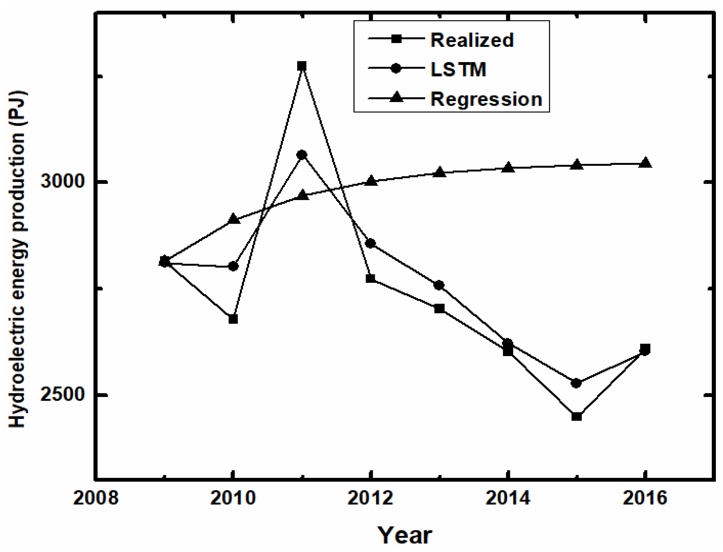
On yearly basis, the LSTM projected HE-EP for 2009 as ~2810.89 PJ (~0.17% forecast error) and 2010 as ~2801.95 PJ (~4.61% forecast error) for the short-term (see Figure 2). These errors combine to achieve an average short-term forecast error of ~2.39% and accuracy of ~97.61% as shown in Table 1. Yearly forecast results for the 2011–2013 medium-term period also achieve considerably high accuracy. The forecast output on HE-EP of ~2856.07 PJ and ~2757.16 PJ for 2012 and 2013 respectively all achieve forecast errors of at most 3%; i.e., ~2.98% for 2012 and ~1.99% for 2013. An ~6.36% forecast error on HE-EP for 2011 contributed to the 3.78% average error for the medium-term and with corresponding accuracy of 96.22% as shown in Table 1. The long-term projections on HE-EP are also of high accuracy of at least 96%; ~2621.89 PJ (~99.25% accuracy) for 2014, ~2528.70 PJ (~96.74% accuracy) for 2015 and ~2603.60 PJ (~99.81% accuracy) for 2016 with average forecast error and accuracy of 1.40% and 98.60% respectively (see Table 1). On the average, the LSTM-based forecast on HE-EP achieves accuracy of 96.46% or better on the eight-year period with MAD of 72.160, MAPE of 2.539 and RMSE of 96.916. Relative to results from the linear regression, our LSTM technique achieves higher accuracy. The accuracy of the regression output for short-term projections is high but deviates massively in the medium and long terms. Overall, the forecast error indexes from utilizing the linear regression technique for all eight years are a MAD of 318.293, MAPE of 11.947 and RMSE of 358.453 (see Table 1). Thus, using the MAPE index our technique presents improvements of ~5-fold.
Due to the high energy efficiency in utilizing hydroelectric power, there is not much difference in the accuracies for production and consumption. As depicted on Figure 3, the forecast output from utilizing the LSTM technique predicts monthly hydroelectric energy consumption (HE-EC) at a high accuracy. In the very short-run the results depict striking accuracy as the LSTM-outputs ~300.62 PJ as HE-EC for June 2009 with actual value of ~301.03 PJ; thus, achieving forecast accuracy of ~99.86%. Output for mid-short-run also achieves high forecast accuracy to the magnitude of ~98.68%; [i.e., forecast output on HE-EC for January 2010 of ~233.44 PJ and actual of ~230.39 PJ]. Monthly predictions for medium and long terms are equally of high accuracy; HE-EC in December 2013 and September 2016 were predicted to be ~210.17 PJ and ~159.64 PJ respectively with accuracies of ~98.82% and ~99.73%.
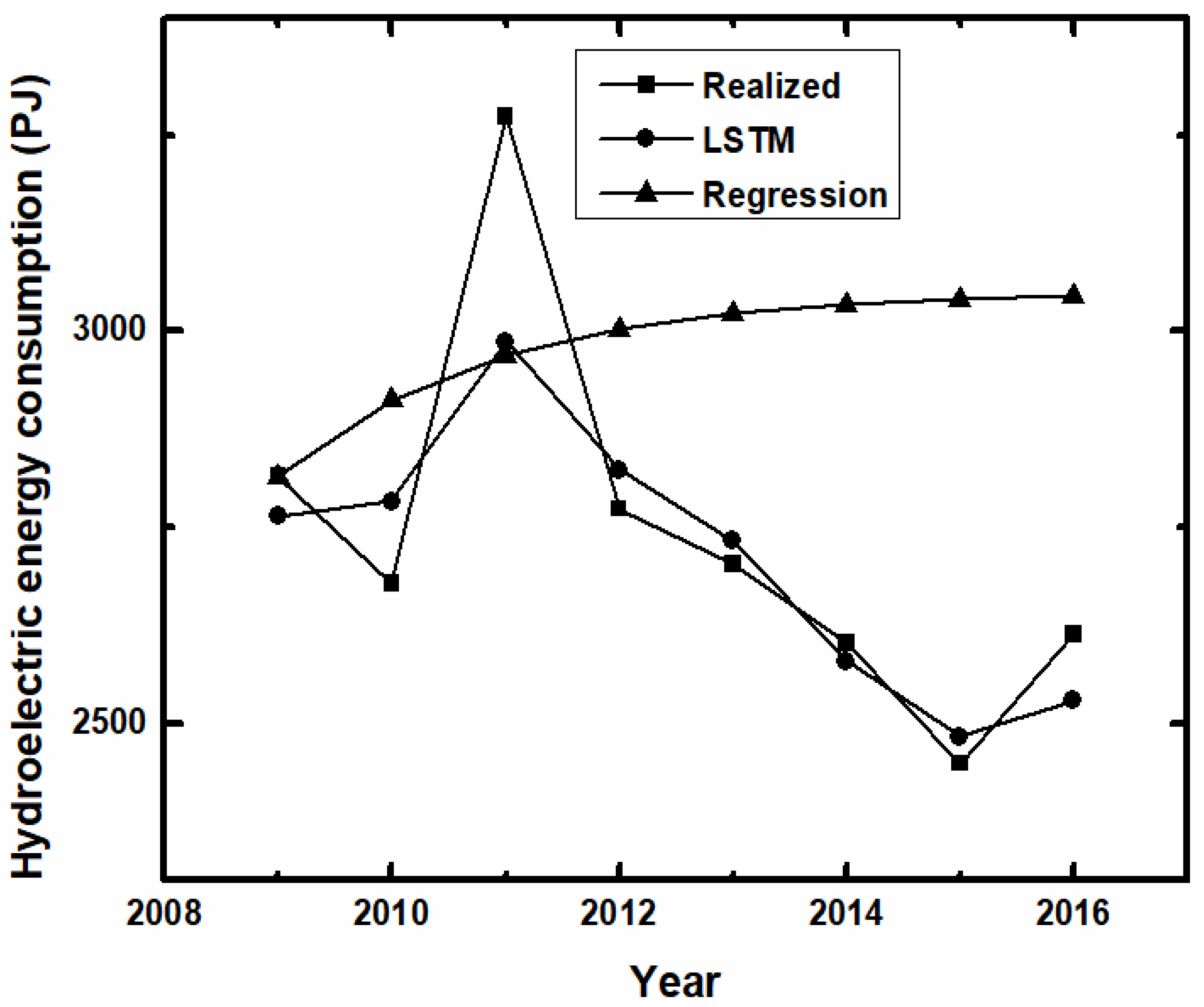
Just as in the monthly case, the identical production and consumption data reflects in the similarity in forecast output, error and accuracy in HE-EC. On yearly basis, the LSTM projected HE-EC for 2009 as ~2764.36 PJ (an undercast of ~1.82%) and 2010 as ~2783.17 PJ (an overcast of ~3.92%) for the short-term (see Figure 4) which combine to reach an average short-term forecast error of ~2.87% and accuracy of ~97.13% as shown in Table 2. Yearly forecast results for the 2011–2013 medium-term period also achieve considerably high accuracy with output on HE-EC of ~2823.99 PJ (overcast of ~1.82%) and ~2733.25 PJ (overcast of ~1.10%) for 2012 and 2013 respectively and forecast errors of at most 2%. An undercast of ~8.76% on HE-EC for 2011 contributed to the 3.90% average forecast error for the medium-term with corresponding accuracy of 96.10% as shown in Table 2. The LSTM-led long-term projections on HE-EC are also of high accuracy up to 99.2%; ~2579.83 PJ (~99.23% accuracy) for 2014, ~2483.82 PJ (~98.58% accuracy) for 2015 and ~2529.87 PJ (~96.80% accuracy) for 2016 with corresponding average forecast error and accuracy of 1.83% and 98.17% respectively (see Table 2). The LSTM-based projections on HE-EC achieves average forecast accuracy of 97.13% or better on HE-EC for the eight-year period with MAD of 83.074, MAPE of 2.865 and RMSE of 116.229. Comparatively, our LSTM technique achieves higher accuracy than utilizing a linear regression. Though the accuracy of the regression technique for short-term projections is high the overall forecast error indexes for the eight-year period are considerably high; with a MAD of 317.657, MAPE of 11.918 and RMSE of 357.683 (see Table 2). Using the MAPE index as a benchmark our technique presents improvements of ~4-fold.
3.2. Renewable Energy Supply from Biomass Sources, US
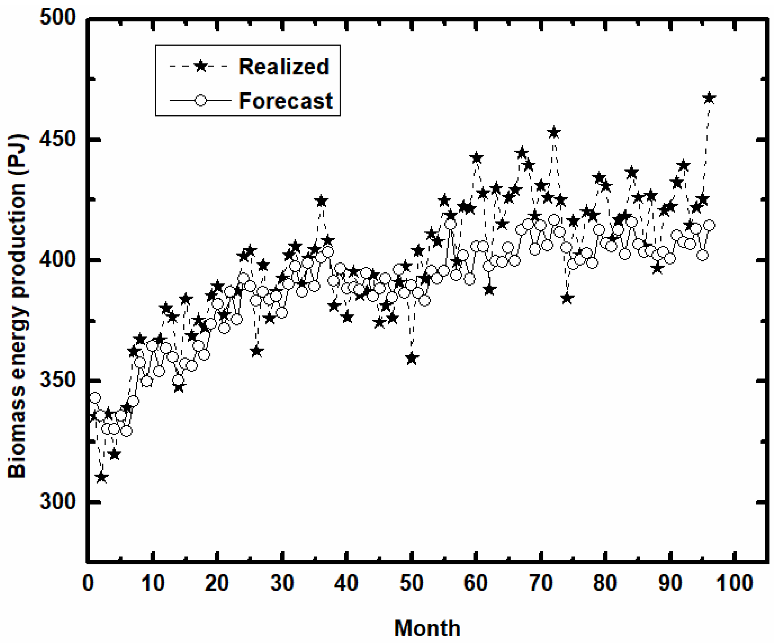
We achieve high forecast accuracy in forecasting monthly renewable energy production from biomass sources (REP-BMs). As depicted on Figure 5 the forecast curve closely mimics the observed consumption levels. The proposed LTSM technique projected REP-BMs for October 2009, a period equally considered as very short-run, as ~364.45 PJ at an accuracy of ~99.80% (an undercast of ~0.20%). LSTM forecast output of ~371.76 PJ for September 2010 presents a marginal deviation of ~5.90 PJ from its observed value of ~377.66 PJ, hence a forecast error of ~1.56% and an accuracy of ~98.44%. Likewise, medium and long term monthly REC-BMs forecasts depict high accuracies to as high as 99.85% (an overcast of ~0.57 PJ) for March 2012 and 99.35% (an undercast of ~2.64 PJ) for February 2016.
For all yearly projections of REC-BMs, the LSTM-based technique reaches a minimum forecast error of ~0.82% (an undercast of ~34.34 PJ for 2009) and maximum of ~4.9% (an undercast of ~252.53 PJ for 2014) for the entire 2009–2016 forecast period (see Figure 6). The yearly absolute forecast errors of ~0.82% for 2009 and ~2.69% for 2010 combine to achieve an average of 1.76% for short-term with corresponding 98.24% forecast accuracy as depicted in Table 3. We achieve forecast accuracies of ~97% or better for the overall eight-year period considering a MAD of 133.051, a MAPE of 2.708 (accuracy of ~97.29%) and RMSE of 152.129 (see Table 3). Thus, results from the LSTM technique straddle that from linear regression (see Figure 6) as the latter reported a MAD of 1272.130, a MAPE of 26.047 (accuracy of ~73.95%) and RMSE of 1358.028 for the 2009–2016 forecast period (see Table 3).
We also achieve high accuracy in forecasting monthly renewable energy consumption from biomass sources (REC-BMs). As depicted in Figure 7 the forecast output (represented by the solid-star curve) closely imitates the observed consumption (dotted-line) levels. Similar to the case of HE-EC the proposed LTSM technique projected REC-BMs for November 2009, a period equally considered as part of the very short-run, as ~359.69 PJ at an accuracy of ~99.42%. Forecast output of ~382.47 PJ for July 2010 deviated marginally from its observed value by ~0.91% and achieves accuracy of ~99.09%. Medium and long term monthly REC-BMs forecasts are likewise of high accuracy to as high as 99.15% (an overcast of ~3.30 PJ) for March 2012 and 99.70% (an undercast of 1.23 PJ) for September 2016.
On yearly projections of REC-BMs, the LSTM-based technique achieves minimum forecast error ~0.21% (undercast of ~9.75 PJ for 2010) and maximum of ~3.5% (undercast of ~179.28 PJ for 2014) for the entire 2009–2016 forecast period (see Figure 8). The yearly absolute forecast errors of ~1.68% for 2009 and ~0.21 for 2010 combine to achieve an average of 0.95% for short-term with corresponding 99.05% forecast accuracy as depicted in Table 2. We recorded yearly forecast accuracy of 98.32% and 97.30% for medium and long-term respectively (see Table 4). We achieve forecast accuracies of 97% or better for the overall eight-year period considered with MAD of 91.401 (accuracy of 98.07%), MAPE of 1.883 (accuracy of ~98.12%) and RMSE of 107.128 (accuracy of 97.74%) (see Table 4). Based on results from utilizing a linear regression technique (see Figure 8), a MAD of 1221.053, a MAPE of 25.189 (accuracy of ~74.81%) and RMSE of 1308.052 for the 2009–2016 forecast period (see Table 4) shows that the LSTM-RNN technique present improvement of ~13-fold.
3.3. Total Primary Renewable and Energy Supply, Selected Regions
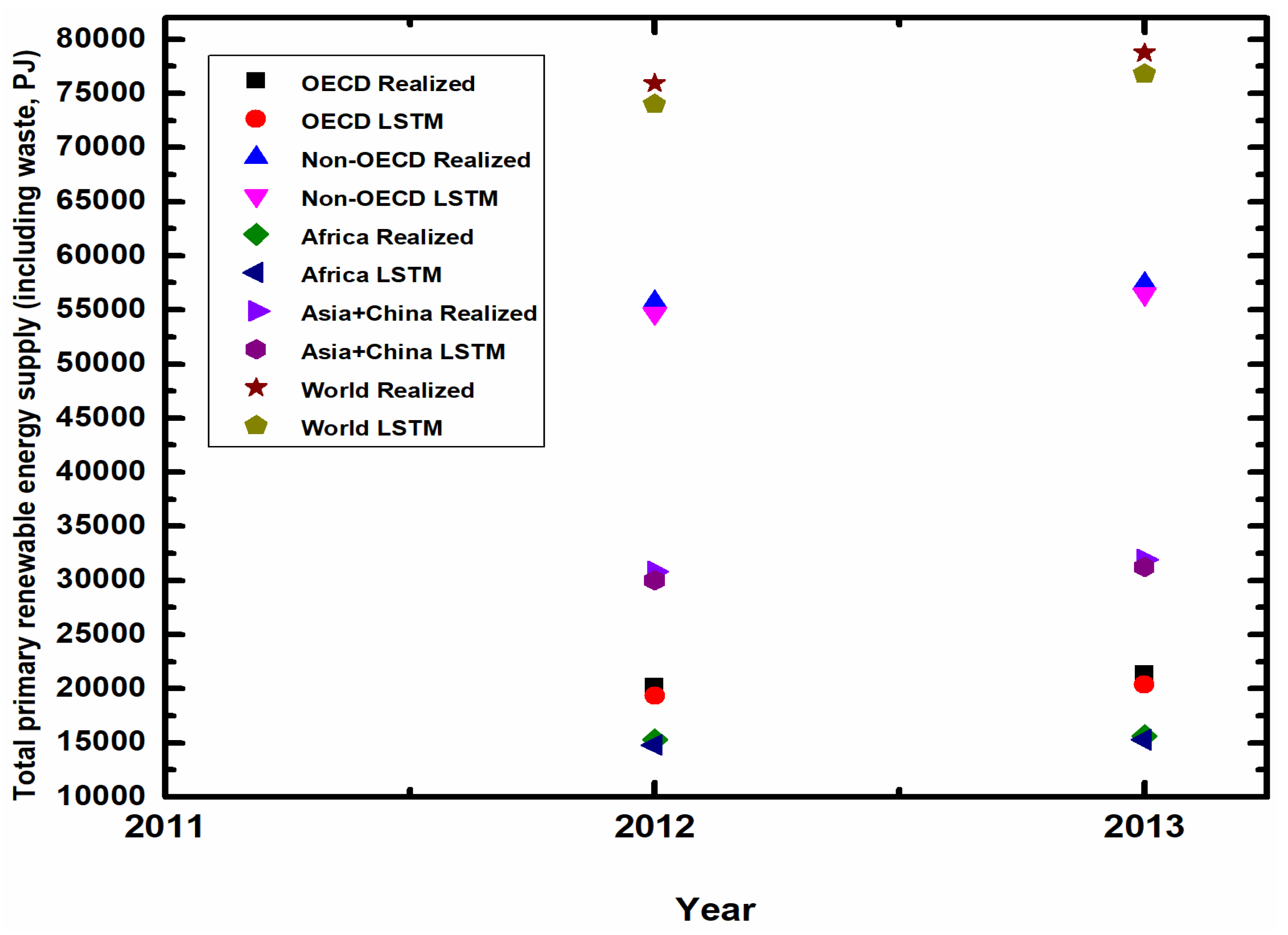
The difficulty in replicating existing well-established renewable energy forecasting models to other countries has been a daunting task to modelers. The characteristics of each geographic region and sectors necessitate separate modules per region but the LSTM-RNN-based model can be replicated to other regions. We test the replicability and applicability to other regions other than the US by utilizing the proposed model to forecast total renewable and waste energy supply (TRAWES) in OECD countries, non-OECD countries, Africa, Asia (including China) and the world as a whole. Using yearly data from IEA for 1990–2010 as training set and 2011 as test set, we make short-term projections for these regions for 2012 and 2013 and the results are depicted in Figure 9.
As depicted in Figure 9, the close proximity of results from the proposed LSTM-RNN own-data-driven modeling technique (i.e., LSTM) to the observed (i.e., Realized) levels for all regions depict the high accuracy of the technique for these regions. The LSTM projections of TRAWES for Africa were reported as ~14793.54 PJ (forecast accuracy of ~96.71%) for 2012 and ~15266.04 PJ (forecast accuracy of ~97.57%) for 2013 with average forecast error of ~2.86% for the two-year period. With the inclusion of China in the Asian region, renewable energy demand has increased astronomically due to the massive energy demand in China and China’s policy to cut down on energy-related greenhouse gas emissions with the use of renewable energy, which leads to extensive volatility in renewable energy forecasting. Despite such variability and volatility, the LSTM-RNN-based projections on TRAWES for Asia achieve high accuracies up to ~97.40% for the ~30007.60 PJ forecast in 2012 and ~97.88% for the ~31248.99 PJ estimated in 2013. The achieved high accuracy also applies to OECD countries, non-OECDs and the world. The average absolute forecast error for OECD countries, non-OECDs and the world for the two-year 2012–2013 period are ~4.37%, ~1.75% and ~2.49% respectively which depict forecast accuracies of ~96, ~ 98% and ~98% for the three regions respectively.
4. Discussions
The zero-assumptions, no assumption-driven independent variables, combined with the high-performing LSTM RNN technique adopted in this study resulted in high and sustained accuracy in renewable energy forecasting. The effect of causal variables (CVs) such as economic growth, world oil price and technology and their related assumptions were all not considered hence the variability and dynamism in CVs as well as unrealized assumptions did not affect the accuracy of the variables used in this study.
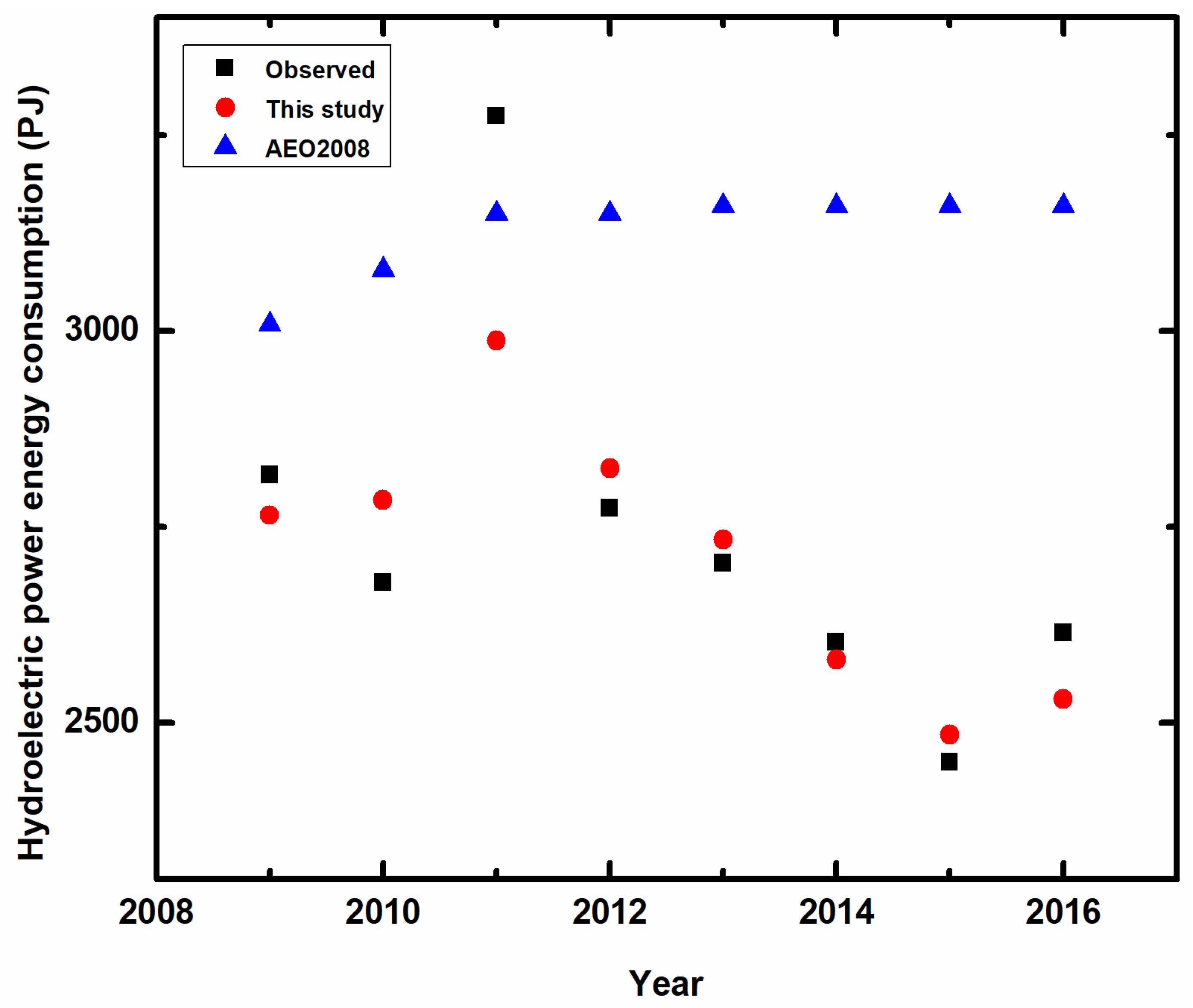
On projections of hydroelectric power consumption, the forecast error of ~1.83% for 2009 presents improvement of ~3.73-fold on the ~3007.64 PJ (see Figure 10) reported in AEO2008 from utilizing the NEMS. Results from the LSTM RNN-based forecast of ~2823.89 PJ for 2012, ~2733.25 PJ for 2013, ~2579.83 PJ for 2014, ~2483.82 PJ for 2015 and ~2529.87 PJ for 2016 (see Figure 10) correspond to improvements of ~7.4-fold, ~15.3-fold, ~24.7-fold, ~20.4-fold and ~6.5-fold respectively on AEO2008 projections. The forecast errors from AEO2008 projections on HE-EC for short, medium and long terms are ~10.86%, ~11.40% and ~23.73% respectively with corresponding overall error indexes of ~419.65 for MAD, ~15.89 for MAPE and ~456.89 for RMSE. Comparatively, the LSTM RNN-based forecast present improvement of ~7.99pp [~3.78-fold] for short-term, ~7.50pp [~2.92-fold] for medium-term, ~21.90pp [~12.97-fold] for long-term and ~5.55-fold [using MAPE] for the overall 2009–2016 period. The cumulative cost due to forecast error in utilizing our proposed LSTM RNN technique for the 8-year forecast period is ~664.59 PJ which is significantly less than the ~3357.21 PJ from utilizing the NEMS AEO2008 forecast; thus, our approach saves the United States ~2692.62 PJ. Due to the similarities in the HE-EC and HE-EP data, we also record high and improved forecast accuracies in HE-EP projections.
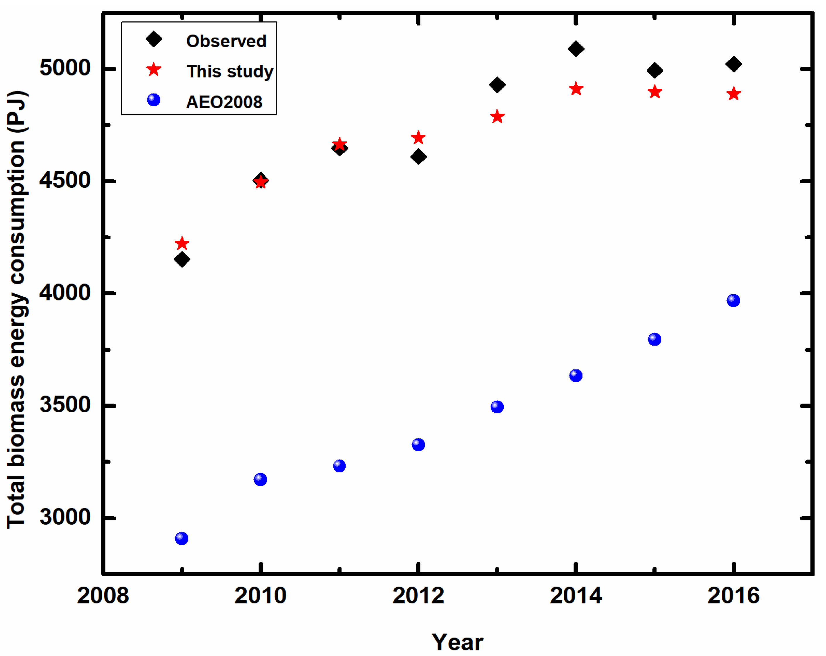
We also achieve enormous improvement on projections of total biomass energy consumption. It is evident in Figure 11 that our LSTM RNN-based forecast results on REC-BMs is relatively close to the observed values than projections in AEO2008. Results from AEO2008 consistently underestimated REC-BMs for all the 8-year forecast period. Results on REC-BMs from the LSTM RNN-based forecast of ~4222.57 PJ (~1.68% error) for 2009, ~4495.15 PJ (~0.21% error) for 2010, ~4664.22 PJ (~0.35% error) for 2011, ~4693.32 PJ (~1.82% error) for 2012, ~4787.99 PJ (~2.89% error) for 2013, ~4910.98 PJ (~3.52% error) for 2014, ~4898.08 PJ (~1.94% error) for 2015 and ~4888.70 PJ (~2.66% error) for 2016 (see Figure 11) correspond to improvements [in fold] of ~17.83, ~138.26, ~87.28, ~15.34, ~10.09, ~8.12, ~12.41 and ~7.90 respectively on AEO2008 projections. Forecast errors on REC-BMs from AEO2008 projections for short, medium and long terms are ~29.79%, ~29.15% and ~24.55% respectively; with resultant MAD, MAPE and RMSE indexes of ~1303.29, ~27.59 and ~1309.57 respectively. Relatively, our LSTM RNN-based forecast technique present improvement of ~28.84pp [~31.34-fold] for short-term, ~27.47pp [~17.35-fold] for medium-term, ~21.85pp [~9.09-fold] for long-term and ~14.65-fold [using MAPE] on REC-BMs for the 2009–2016 period. The aggregate cost on REC-BMs due to forecast error from utilizing LSTM RNN technique is ~731.21 PJ for the 8-year period which is ominously less than the ~10426.29 PJ from utilizing the NEMS AEO2008 forecast; thus, our approach saves the United States ~9695.09 PJ. The identical data set for REC-BMs and REP-BMs spills over to equally high forecast accuracy and significant improvement in REP-BMs projections.
Though variability in renewable energy data varies per region, the LSTM-based own-data-driven technique achieves high accuracy in OECD, non-OECD, Africa, Asia and the world as whole on total renewable and waste energy supply forecasting. Forecast results on TRAWES for high renewable demand regions including OECD and Achieve all achieve high accuracies up to ~98% for the short term.
5. Conclusions
The use of renewable energy as an environmentally-friendly and sustainable source of energy as a viable option to minimizing energy-related greenhouse gas emissions is prerequisite to achieving set intended nationally determined contributions (INDCs) and policymakers rely on high accuracy forecasts in designing and implementing realistic energy policies. However existing and well-established energy demand forecasting models, such as NEMS, require vast [endogenous and exogenous] independent variables and massive assumptions in making projections which has spilled-over to high inaccuracies in past AEO projections on renewable energy demand and generation in the United States and the world. Existing high-profile renewable energy demand forecasting models require vast independent variables including GDP, population, prices of renewable energies, prices of fossil fuels, etc. In order to capture the effects of such independent variables, the future trends of these variables must be assumed which usually deviate from realized values. Thus, the weight of such assumptions on the accuracy of projections cannot be ignored. In this article, we contribute to improving the accuracy of renewable energy demand forecasting by creating and implementing a comparatively high accuracy LSTM RNN forecasting algorithm that requires no independent variables and assumptions for total biomass and hydroelectric energy demand and generation forecasting. We contribute to literature by proposing and implementing a forecasting technique that requires none of such independent variables as well as their related assumptions for renewable energy forecasting.
Existing models are also usually developed for a single time horizon (short, medium or long term) forecasting and the inaccuracy for the short-term and medium-term related outputs from the long-term forecasts are substantially high. We also contribute to literature as the short-term-related as well as medium-term-related outputs from our long-term forecast are all of relatively high accuracy and thus, sustainable and present significant improvement in accuracy of existing high-profile models. Our forecast results on renewable energy production and consumption from biomass sources (REP-BMs and REC-BMs) and hydroelectric power energy supply and demand (HE-EP and HE-EC) show that the independent-variable-free and assumption-free LSTM RNN technique present enormous improvement on reference case projections in EIA’s AEO2008 for short, medium and long terms. The cumulative cost due to forecast error in utilizing our forecasting technique is ~664.59 PJ for hydroelectric power energy consumption, which is ~2692.62 PJ less than that from AEO2008 reference case projections; and ~731.21 PJ for total biomass energy consumption, which is ~9695.09 PJ less than AEO2008 reference case projections.
Existing models are also developed for a particular geographic region due to the unique characteristics of each region and/or sector hence replicability to other countries, regions and sectors are usually challenging. In addition to the zero-independent variables, zero-assumptions and sustainable high-accuracy time-horizon nature, our model can be replicated to other countries, regions, sectors and subsectors though differing high accuracy levels could be achieved per region as the data characteristics differ per region as depicted in Section 3.3 above. Future studies could extend the technique to other sources of energy as well as other individual countries.
Lastly, implementing our technique for future renewable energy forecasting suggests substantial revisions of forecast output of business-as-usual and reference case projections from utilizing existing models.
Acknowledgments
This paper is supported by the National Natural Science Foundation of China (No. 71774026).
Author Contributions
Authors Amos Oppong and Jie Ma conceived the idea; Kingsley Nketia Acheampong wrote the algorithm; Amos Oppong, Jie Ma, Kingsley Nketia Acheampong and Lucille Aba Abruquah designed, prepared and revised the paper.
Conflicts of Interest
Authors declare no conflict of interest. Authors declare that the sponsors had no role in the conception, design, preparation and revision of the manuscript and in the decision to publish the results.
Appendix A. Steps to Developing and Utilizing the Zero Assumption LSTM RNN Forecasting Technique
First, we imported all of the functions and classes we intend to use. This assumes a working SciPy environment with the Keras deep learning library installed. Before doing any rigorous tasks, it is a good idea to fix the random number seed to ensure our results are reproducible.
Then, we loaded the dataset as a Pandas dataframe. We then extracted the NumPy array from the dataframe and convert the integer values to floating point values, which are more suitable for modeling with a neural network.
As a matter of fact, LSTMs are sensitive to the scale of the input data, specifically when the sigmoid or tanh activation functions are used. With this notion in mind, we rescale the data to the range of 0-to-1, this is usually called normalizing. We normalized the dataset using the MinMaxScaler preprocessing class from the scikit-learn library.
After that, we modelled the data and estimated the performance of our model on the training dataset, simply because, we needed to get an idea of the performance of the model on a new unseen data. With the nature of our data, we used the cross-validation approach.
Because of phrasing our data as a time series data, the sequence of values was very important to us. Therefore, we split the ordered M dataset into train and test datasets. Our model calculates the index of the split point and separates the data into the training datasets with k of the observations that we can use to train our model, leaving the remaining M – k for testing the model.
With the above established, we proceeded to create how the model should perceive the data during training and testing. We loaded our data sequentially according to the date, into a NumPy array that we would convert into a dataset for our model and the window, which is the number of previous time steps to use as input variables to predict a next time’s period, which in our model, the windows vary.
The LSTM network expects the input data X to be provided with a specific array structure in the form of: [samples, time steps, features]. At this point of our implementation, our data is in the form: [samples, features] and we are framing the problem as l time step (window) for each sample. So, we transformed the prepared train and test input data into the expected structure using a numpy.reshape().
After this, we were ready to design and fit our LSTM network for our renewable energy problem. Our model’s network has a visible layer with 1 input, a hidden layer with n LSTM blocks or neurons and an output layer that makes a single value prediction. The default sigmoid activation function is used for the LSTM blocks. The network is trained for 300 epochs and a batch size of q was used.
Once the model is fit, we estimate the performance of the model on the train and test datasets. This will give us a point of comparison for new models. Also, we inverted the predictions before calculating error scores to ensure that performance is reported in the same units as the original data.
Finally, we generated the predictions using the model for both the train and test dataset to get a visual indication of the skill of the model. Because of how the dataset we prepared, we must shift the predictions so that they align on the x-axis with the original dataset. Once prepared, the data is plotted, showing the original dataset in blue, the predictions for the training dataset in green and the predictions on the unseen test dataset in red.
References
- Rogelj, J.; Schaeffer, M.; Friedlingstein, P.; Gillett, N.P.; van Vuuren, D.P.; Riahi, K.; Allen, M.; Knutti, R. Differences between carbon budget estimates unravelled. Nat. Clim. Chang. 2016, 6, 245–252. [Google Scholar] [CrossRef] [Green Version]
- Sachs, J.D.; Schmidt-traub, G.; Williams, J. Pathways to zero emissions. Nat. Geosci. 2016, 9, 799. [Google Scholar] [CrossRef]
- Meinshausen, M.; Jeffery, L.; Guetschow, J.; Robiou du Pont, Y.; Rogelj, J.; Schaeffer, M.; Höhne, N.; den Elzen, M.; Oberthür, S.; Meinshausen, N. National post-2020 greenhouse gas targets and diversity-aware leadership. Nat. Clim. Chang. 2015, 1306, 1–10. [Google Scholar] [CrossRef]
- Watson, R.T.; Rodhe, H.; Oeschger, H.; Siegenthaler, U. Greenhouse gases and aerosols. Clim. Chang. IPCC Sci. Assess. 1990, 1, 17. [Google Scholar]
- Solomon, S.; Daniel, J.S.; Sanford, T.J.; Murphy, D.M.; Plattner, G.-K.; Knutti, R.; Friedlingstein, P. Persistence of climate changes due to a range of greenhouse gases. Proc. Natl. Acad. Sci. USA 2010, 107, 18354–18359. [Google Scholar] [CrossRef] [PubMed]
- Montzka, S.A.; Dlugokencky, E.J.; Butler, J.H. Non-CO2 greenhouse gases and climate change. Nature 2011, 476, 43–50. [Google Scholar] [CrossRef] [PubMed]
- Tian, H.; Lu, C.; Ciais, P.; Michalak, A.M.; Canadell, J.G.; Saikawa, E.; Huntzinger, D.N.; Gurney, K.R.; Sitch, S.; Zhang, B.; et al. The terrestrial biosphere as a net source of greenhouse gases to the atmosphere. Nature 2016, 531, 225–228. [Google Scholar] [CrossRef] [PubMed] [Green Version]
- Yang, J.; Liu, Q.; Li, X.; Cui, X. Overview of wind power in China: Status and future. Sustainability 2017, 9, 1454. [Google Scholar] [CrossRef]
- Beck, F.; Martinot, E. Renewable energy policies and barriers. Encycl. Energy 2004, 34, 365–383. [Google Scholar]
- Lund, H. Renewable energy strategies for sustainable development. Energy 2007, 32, 912–919. [Google Scholar] [CrossRef]
- Verbruggen, A.; Fischedick, M.; Moomaw, W.; Weir, T.; Nadaï, A.; Nilsson, L.J.; Nyboer, J.; Sathaye, J. Renewable energy costs, potentials, barriers: Conceptual issues. Energy Policy 2010, 38, 850–861. [Google Scholar] [CrossRef]
- Panwar, N.L.; Kaushik, S.C.; Kothari, S. Role of renewable energy sources in environmental protection: A review. Renew. Sustain. Energy Rev. 2011, 15, 1513–1524. [Google Scholar] [CrossRef]
- Kandpal, T.C.; Broman, L. Renewable energy education: A global status review. Renew. Sustain. Energy Rev. 2014, 34, 300–324. [Google Scholar] [CrossRef]
- Franzitta, V.; Curto, D.; Rao, D. Energetic sustainability using renewable energies in the mediterranean sea. Sustainability 2016, 8, 1164. [Google Scholar] [CrossRef]
- Li, S.; Li, R. Comparison of forecasting energy consumption in Shandong, China Using the ARIMA model, GM model and ARIMA-GM model. Sustainability 2017, 9, 1181. [Google Scholar] [CrossRef]
- O’Neill, B.C.; Desai, M. Accuracy of past projections of US energy consumption. Energy Policy 2005, 33, 979–993. [Google Scholar] [CrossRef]
- Gilbert, A.Q.; Sovacool, B.K. Looking the wrong way: Bias, renewable electricity and energy modelling in the United States. Energy 2016, 94, 533–541. [Google Scholar] [CrossRef]
- Strachan, N.; Fais, B.; Daly, H. Reinventing the energy modelling–policy interface. Nat. Energy 2016, 1, 16012. [Google Scholar] [CrossRef]
- The National Energy Modeling System: An Overview 2009; DOE/EIA-0581; U.S. Energy Information Administration, Office of Integrated Analysis and Forecasting, US Department of Energy: Washington, DC, USA, 2009; Volume DOE/EIA-05.
- Annual Energy Outlook 2002 with Projections to 2020; U.S. Energy Information Administration: Washington, DC, USA, 2002; Volume DOE/EIA-03.
- Inman, R.H.; Pedro, H.T.C.; Coimbra, C.F.M. Solar forecasting methods for renewable energy integration. Prog. Energy Combust. Sci. 2013, 39, 535–576. [Google Scholar] [CrossRef]
- Foley, A.M.; Leahy, P.G.; Marvuglia, A.; McKeogh, E.J. Current methods and advances in forecasting of wind power generation. Renew. Energy 2012, 37, 1–8. [Google Scholar] [CrossRef] [Green Version]
- Tang, L.; Yu, L.; He, K. A novel data-characteristic-driven modeling methodology for nuclear energy consumption forecasting. Appl. Energy 2014, 128, 1–14. [Google Scholar] [CrossRef]
- Gers, F.A.; Schraudolph, N.N.; Schmidhuber, J. Learning precise timing with LSTM recurrent networks. J. Mach. Learn. Res. 2002, 3, 115–143. [Google Scholar] [CrossRef]
- Wöllmer, M.; Kaiser, M.; Eyben, F.; Schuller, B.; Rigoll, G. LSTM-modeling of continuous emotions in an audiovisual affect recognition framework. Image Vis. Comput. 2013, 31, 153–163. [Google Scholar] [CrossRef]
- Milone, D.; Pitruzzella, S.; Franzitta, V.; Viola, A.; Trapanese, M. Energy savings through integration of the illumination natural and artificial, using a system of automatic dimming: Case study. Appl. Mech. Mater. 2013, 372, 253–258. [Google Scholar] [CrossRef]
- U.S. Energy Information Administration. Monthly Energy Review. Available online: https://www.eia.gov/totalenergy/data/monthly/ (accessed on 4 October 2017).
- International Energy Agency. Unit Converter. Available online: https://www.iea.org/statistics/resources/unitconverter/ (accessed on 1 March 2017).
- Assumptions to the Annual Energy Outlook 2015; U.S. Department of Energy, U.S. Energy Information Administration: Washington, DC, USA, 2015.
- Hamzaçebi, C. Forecasting of Turkey’s net electricity energy consumption on sectoral bases. Energy Policy 2007, 35, 2009–2016. [Google Scholar] [CrossRef]
- Annual Energy Outlook 2008 With Projections to 2030; DOE/EIA-0383; U.S. Energy Information Administration: Washington, DC, USA, 2008; Volume DOE/EIA-03.
Figure 1.
Forecast (i.e., LST) and observed (i.e., Realized) monthly renewable energy production from hydroelectric power source. Data cover the period January 2009 to December 2016.
Figure 1.
Forecast (i.e., LST) and observed (i.e., Realized) monthly renewable energy production from hydroelectric power source. Data cover the period January 2009 to December 2016.
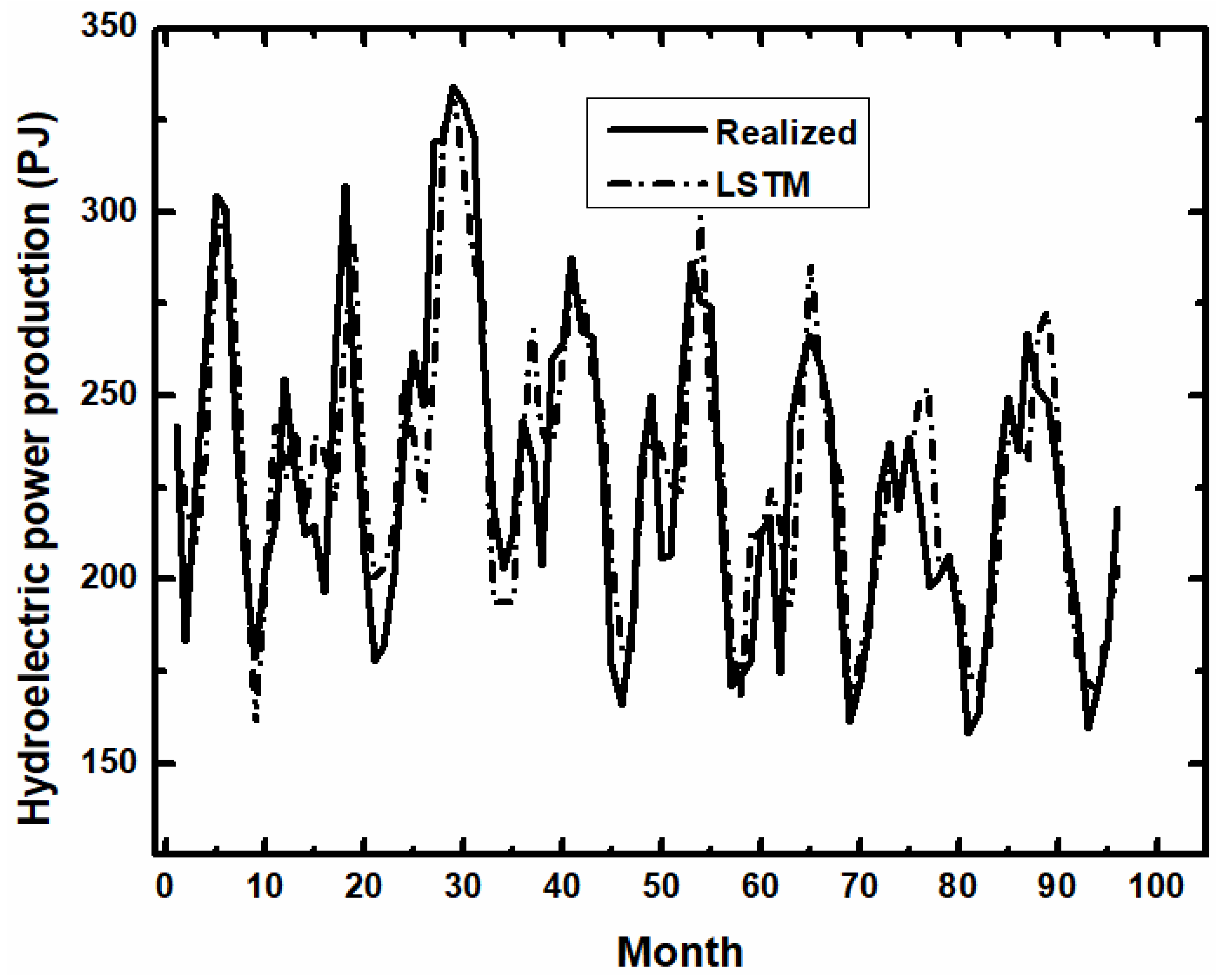
Figure 2.
Comparison of LSTM and linear regression forecasting output of yearly renewable energy production from hydroelectric power sources. Data cover the period of 2009 to 2016.
Figure 2.
Comparison of LSTM and linear regression forecasting output of yearly renewable energy production from hydroelectric power sources. Data cover the period of 2009 to 2016.

Figure 3.
Forecast (i.e., LSTM) and observed (i.e., Realized) monthly renewable energy consumption from hydroelectric power sources. Data cover the period January 2009 to December 2016.
Figure 3.
Forecast (i.e., LSTM) and observed (i.e., Realized) monthly renewable energy consumption from hydroelectric power sources. Data cover the period January 2009 to December 2016.
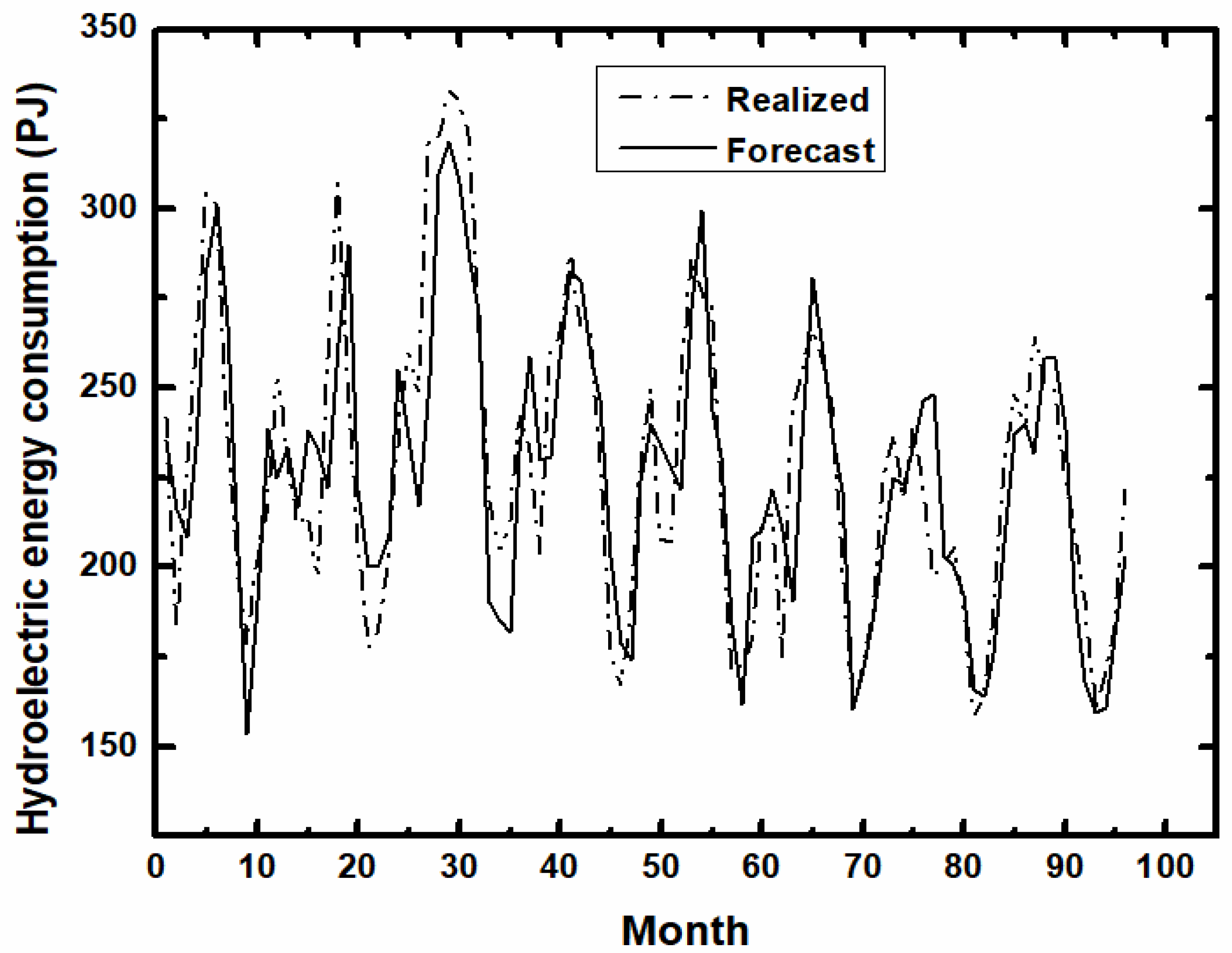
Figure 4.
Comparison of LSTM and linear regression forecasting output of yearly renewable energy consumption from hydroelectric power sources. Data cover the period of 2009 to 2016.
Figure 4.
Comparison of LSTM and linear regression forecasting output of yearly renewable energy consumption from hydroelectric power sources. Data cover the period of 2009 to 2016.

Figure 5.
Forecast and actual monthly renewable energy production from biomass sources for the period January 2009 to December 2016.
Figure 5.
Forecast and actual monthly renewable energy production from biomass sources for the period January 2009 to December 2016.

Figure 6.
Comparison of LSTM and linear regression forecasting output of yearly renewable energy production from biomass sources. Data cover the period of 2009 to 2016.
Figure 6.
Comparison of LSTM and linear regression forecasting output of yearly renewable energy production from biomass sources. Data cover the period of 2009 to 2016.
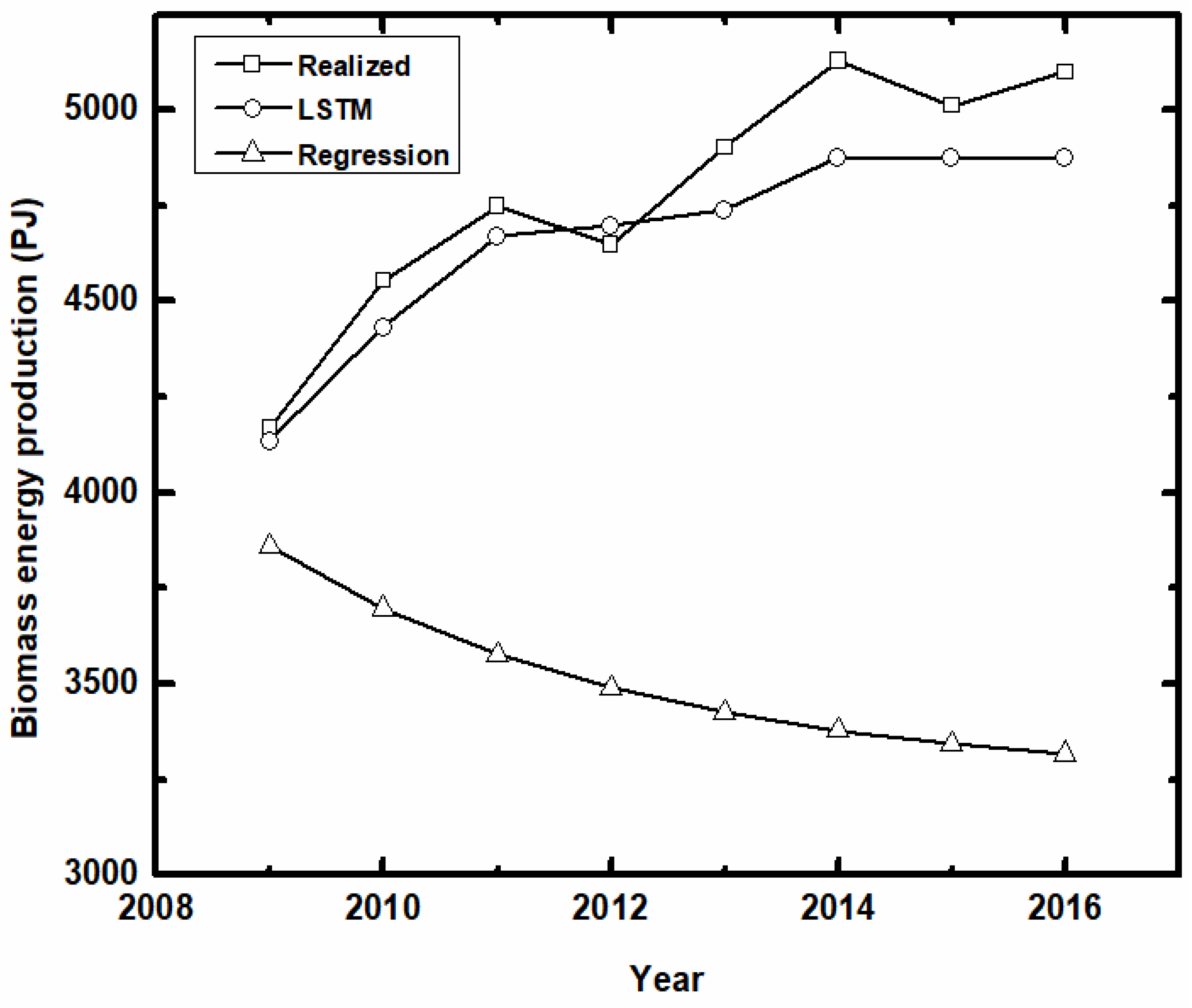
Figure 7.
Forecast and actual monthly renewable energy consumption from biomass sources for the period January 2009 to December 2016.
Figure 7.
Forecast and actual monthly renewable energy consumption from biomass sources for the period January 2009 to December 2016.
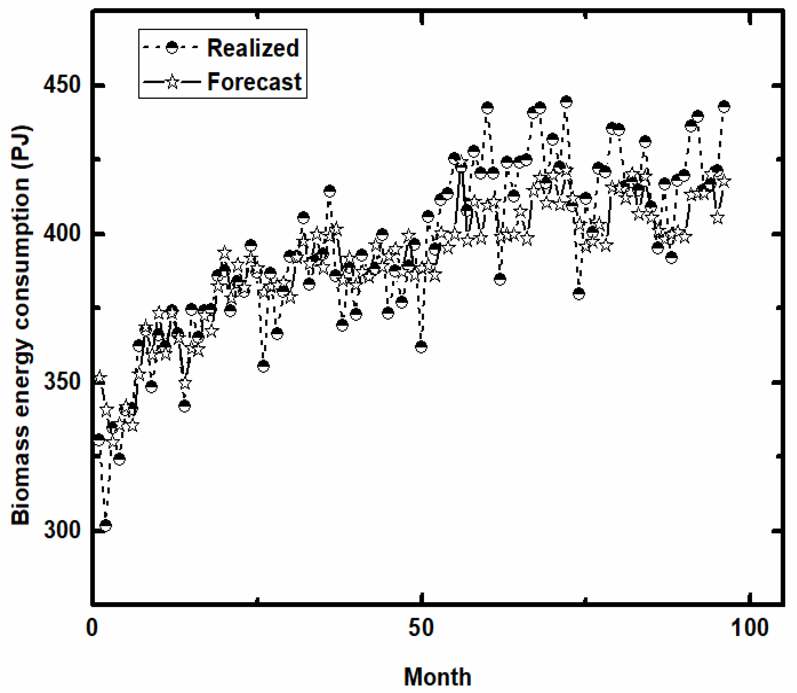
Figure 8.
Forecast and actual yearly renewable energy consumption from biomass sources for the period 2009 to 2016, LSTM vs. linear regression.
Figure 8.
Forecast and actual yearly renewable energy consumption from biomass sources for the period 2009 to 2016, LSTM vs. linear regression.
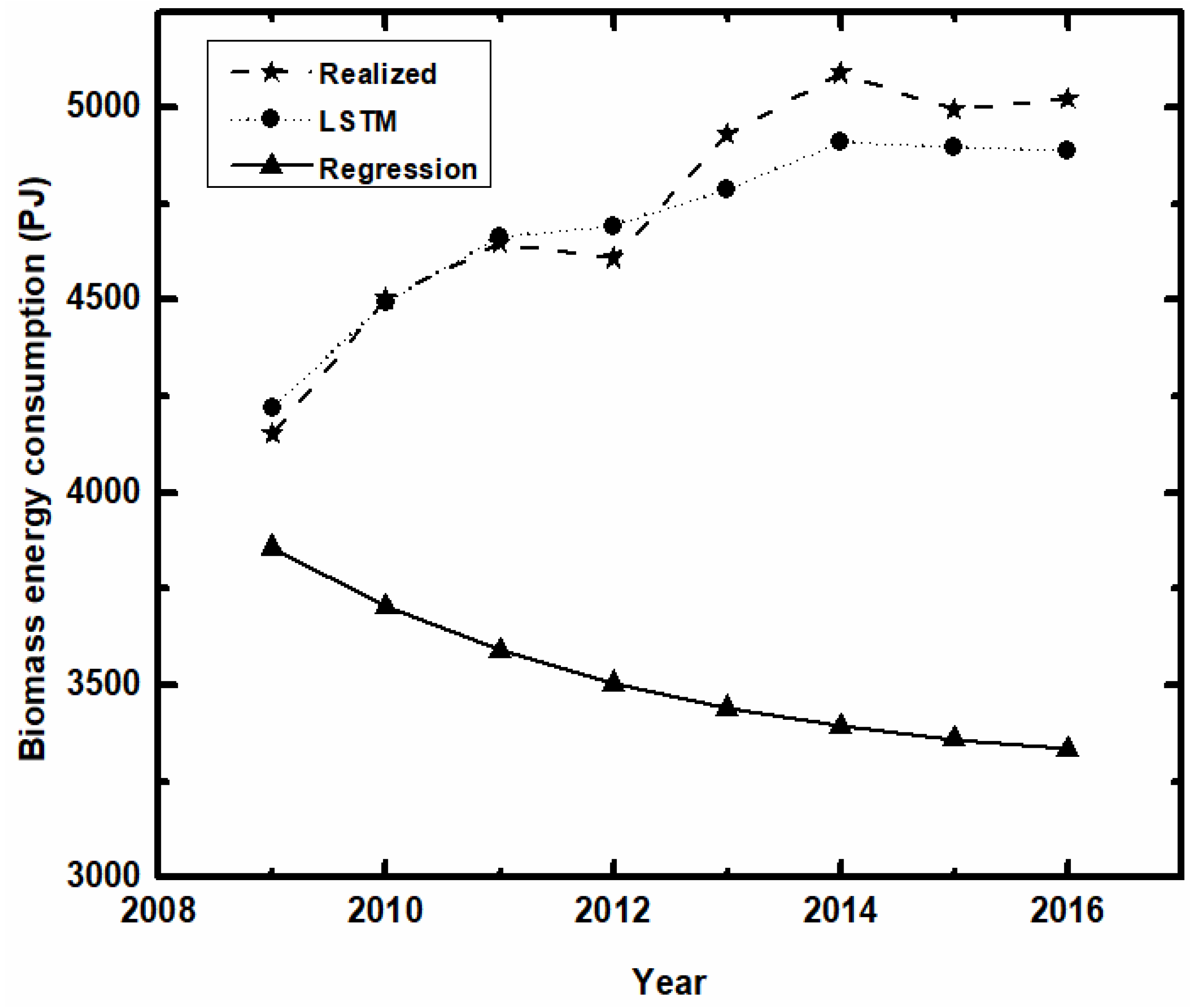
Figure 9.
Projections of yearly total primary renewable and waste energy supply for selected regions, 2012 and 2013, LSTM vs. linear regression.
Figure 9.
Projections of yearly total primary renewable and waste energy supply for selected regions, 2012 and 2013, LSTM vs. linear regression.

Figure 10.
Comparison of forecast results on hydroelectric power energy consumption, LSTM RNN (i.e., this study) vs. NEMS (i.e., AEO2008); energy consumption is measured in PJ.
Figure 10.
Comparison of forecast results on hydroelectric power energy consumption, LSTM RNN (i.e., this study) vs. NEMS (i.e., AEO2008); energy consumption is measured in PJ.

Figure 11.
Comparison of forecast results on total biomass energy consumption, LSTM RNN (i.e., this study) vs. NEMS (i.e., AEO2008); energy consumption is measured in PJ.
Figure 11.
Comparison of forecast results on total biomass energy consumption, LSTM RNN (i.e., this study) vs. NEMS (i.e., AEO2008); energy consumption is measured in PJ.


Table 1.
Forecast error and accuracy on projections of hydroelectric power production.
| Forecast Error | Forecast Accuracy | |
|---|---|---|
| LSTM | ||
| Forecast Horizon | ||
| Short-term | 2.39% | 97.61% |
| Medium-term | 3.78% | 96.22% |
| Long-term | 1.40% | 98.60% |
| Overall Indexes | ||
| MAD | 72.16 | 97.36% |
| MAPE | 2.539 | 97.46% |
| RMSE | 96.916 | 96.46% |
| Linear Regression | ||
| Forecast Horizon | ||
| Short-term | 4.38% | 95.62% |
| Medium-term | 9.79% | 90.21% |
| Long-term | 19.15% | 80.85% |
| Overall Indexes | ||
| MAD | 318.293 | 88.38% |
| MAPE | 11.947 | 88.05% |
| RMSE | 358.453 | 86.91% |
Table 2.
Forecast error and accuracy on projections of hydroelectric power consumption.
| LSTM | Regression | |||
|---|---|---|---|---|
| Forecast Error | Forecast Accuracy | Forecast Error | Forecast Accuracy | |
| Forecast Horizon | ||||
| Short-term | 2.87% | 97.13% | 4.38% | 95.62% |
| Medium-term | 3.90% | 96.10% | 9.79% | 90.21% |
| Long-term | 1.83% | 98.17% | 19.08% | 80.92% |
| Overall Indexes | ||||
| MAD | 83.074 | 96.97% | 317.657 | 88.40% |
| MAPE | 2.865 | 97.13% | 11.918 | 88.08% |
| RMSE | 116.229 | 95.76% | 357.683 | 86.94% |
Table 3.
Forecast error and accuracy on projections of biomass energy production.
| LSTM | Regression | |||
|---|---|---|---|---|
| Forecast Error | Forecast Accuracy | Forecast Error | Forecast Accuracy | |
| Forecast Horizon | ||||
| Short-term | 1.76% | 98.24% | 13.14% | 86.86% |
| Medium-term | 2.02% | 97.98% | 26.58% | 73.42% |
| Long-term | 4.03% | 95.97% | 34.12% | 65.88% |
| Overall Indexes | ||||
| MAD | 133.051 | 97.22% | 1272.130 | 73.40% |
| MAPE | 2.708 | 97.29% | 26.047 | 73.95% |
| RMSE | 152.129 | 96.82% | 1358.028 | 71.61% |
Table 4.
Forecast error and accuracy on projections of biomass energy consumption.
| LSTM | Regression | |||
|---|---|---|---|---|
| Forecast Error | Forecast Accuracy | Forecast Error | Forecast Accuracy | |
| Forecast Horizon | ||||
| Short-term | 0.95% | 99.05% | 12.45% | 87.55% |
| Medium-term | 1.68% | 98.32% | 25.65% | 74.35% |
| Long-term | 2.70% | 97.30% | 33.23% | 66.77% |
| Overall Indexes | ||||
| MAD | 91.401 | 98.07% | 1221.053 | 74.26% |
| MAPE | 1.88 | 98.12% | 25.189 | 74.81% |
| RMSE | 107.128 | 97.74% | 1308.052 | 72.43% |
© 2018 by the authors. Licensee MDPI, Basel, Switzerland. This article is an open access article distributed under the terms and conditions of the Creative Commons Attribution (CC BY) license (http://creativecommons.org/licenses/by/4.0/).
Share and Cite
MDPI and ACS Style
Ma, J.; Oppong, A.; Acheampong, K.N.; Abruquah, L.A. Forecasting Renewable Energy Consumption under Zero Assumptions. Sustainability 2018, 10, 576. https://doi.org/10.3390/su10030576
AMA Style
Ma J, Oppong A, Acheampong KN, Abruquah LA. Forecasting Renewable Energy Consumption under Zero Assumptions. Sustainability. 2018; 10(3):576. https://doi.org/10.3390/su10030576
Chicago/Turabian StyleMa, Jie, Amos Oppong, Kingsley Nketia Acheampong, and Lucille Aba Abruquah. 2018. "Forecasting Renewable Energy Consumption under Zero Assumptions" Sustainability 10, no. 3: 576. https://doi.org/10.3390/su10030576
Note that from the first issue of 2016, this journal uses article numbers instead of page numbers. See further details here.