Standard Data-Based Predictive Modeling for Power Consumption in Turning Machining


1
Graduate School of Management of Technology, Pukyong National University, Busan 48547, Korea
2
Information Technology Laboratory, National Institute of Standards and Technology, Gaithersburg, MD 20899, USA
3
Advanced Manufacturing Office, Office of Energy Efficiency and Renewable Energy, Washington, DC 20585, USA
*
Author to whom correspondence should be addressed.
Sustainability 2018, 10(3), 598; https://doi.org/10.3390/su10030598
Submission received: 15 January 2018
/
Revised: 12 February 2018
/
Accepted: 22 February 2018
/
Published: 26 February 2018
(This article belongs to the Section Sustainable Engineering and Science)
Abstract
:In the metal cutting industry, power consumption is an important metric in the analysis of energy efficiency since it relates to energy consumption of machine tools. Much of the research has developed predictive models that correlate process planning decisions with power consumption through theoretical and/or experimental modeling approaches. These models are created by using the theory of metal cutting mechanics and Design of Experiments. However, these models may lose their ability to predict results correctly outside the required assumptions and limited experimental conditions. Thus, they cannot accurately reflect a diversity of machining configurations; i.e., selections of machine tool, workpiece, cutting tool, coolant option, and machining operation for producing a part, which a machining shop has operated. This paper proposes a predictive modeling approach based on historical data collected from machine tool operations. The proposed approach can create multiple predictive models for power consumption, which can be applicable to the diverse machining configurations. It can create fine-grained models predictable up to the level of a numerical control program. It uses standard-based data interfaces such as STEP-NC and MTConnect to implement interoperable and comprehensive data representations. This paper also presents a case study to demonstrate the feasibility and effectiveness of the proposed approach.
1. Introduction
1.1. Background of Study
In the metal cutting industry, sustainability performance metrics including energy consumption, coolant usage, and disposed waste are emerging as major indicators for improving energy efficiency and reducing environmental burden [1]. Energy consumption is an important metric in sustainability analysis because reducing energy consumption of machine tools can significantly improve the environmental performance of machining operations [2]. In the analysis of energy consumption, a key dominant metric is power consumption, which consists of the machine power consumed by a machine tool’s actions plus the cutting power needed to remove a workpiece [3]. It closely relates to the Specific Energy Consumption (SEC); i.e., the energy consumption for removing a unit-volume material. In turn, the SEC multiplied with Material Removal Rate (MRR) and machining time results in the energy consumption of machining a part [4]. For this reason, significant research has been done to develop predictive models for power consumption in machining. These models enable manufacturers to respond proactively by identifying anticipated power values. They can also provide numerical relationships necessary for predictive control and optimization to improve energy efficiency. Much of the research has modeled the correlation between process planning decisions and the power consumption using theoretical and/or experimental modeling approaches. This correlation comes from the great influence of process planning decisions on the performance of machining operations [5].
A theoretical modeling approach predicts power consumption from the input of process planning decisions using the theory of metal cutting mechanics with some assumptions such as the selection of a linear or nonlinear function for deciding cutting constants [6,7,8,9,10] introduced theoretical models that correlate the power consumption with tool geometry and cutting force. One study proposed a power consumption model based on changes of the SEC and the MRR [3]. Astakhov and Xiao [11] introduced a physics-based principle of minimum strain energy by partitioning energy flows in terms of workpiece, tool and chip, and their interfaces. These works help understand the dependency of power consumption upon cutting force, tool geometries, the MRR, and process parameters such as feed rate, spindle speed, cutting depth, and width. They also provide numerical functions that provide the key inputs to machining power simulators such as the technology presented in [12,13]. However, these theory-based models may not be feasible to predict the result correctly when they cannot provide the correct value for each coefficient of their numerical functions [4].
Meanwhile, an experimental modeling approach relies on actual experiments to make the required predictive models. This approach takes a top-down process that follows Design of Experiments (DOE), machining, data collection, and regression modeling. It can be useful for finding statistical significance in the relationships between process parameters and power consumption [4]. Several studies have used experimental models to build the relationship between the SEC and process parameters using Response Surface Methodology [14], to predict power consumption from MRR without measuring power demand at a machine tool [15], and to characterize the relationship between power consumption and process parameters [4]. Astakhov and Xiao [16] presented a methodology for practical estimation of cutting power with theoretical analysis of cutting force. Helu et al. [17] proposed empirical models to predict energy consumption and to evaluate the trade-offs between environmental and financial impacts. Iqbal et al. [18] presented a rule-based methodology for minimizing energy consumption, maximizing tool life, and maximizing the MRR. Peng and Xu [19] proposed the global, energy-efficient, machining system that includes energy metering, optimization, and data interoperability in the Computer-Aided technology (CAx) chain. Jia et al. [20] introduced a modeling methodology that linked activities, machining states, and the basic unit for energy calculation. Bhinge et al. [21] developed an adaptive prediction model for analyzing the energy usage of a milling machine by Gaussian Process Regression (GPR).
These works [4,14,15,16,17,18,19,20,21] have shown good results in characterizing the numerical relationships between power consumption and process parameters. Also they contribute to create machine-specific models with the use of experimental data, which means the data acquired from small sets of trials assigned by the DOE. However, they have some limitations when being applied to a machine shop due to the following reasons. First, their experiment-based models are only effective within specified, limited, and experimental conditions. The small sets of trials by the DOE do not reflect all machining conditions where a machine tool has operated to produce a number of parts. The change of a Machining Configuration (MC), i.e., the selection of machine tool, workpiece, tool holder, insert, coolant option, and machining operation for producing a designed part, requires another DOE and its associated experimental trials. Specifically, a regression model for one machine tool may not be valid for another machine tool because the model for the latter requires different coefficients. In other words, experiments must be repeated to generate the predictive models that correspond to each MC in the machine shop. Therefore, the experimental approach used to derive individual models may not work well when applied to the entire shop floor.
Second, many of these models are unable to find the relationships between tool path trajectory and power consumption because they focus on the relationships between process parameters and power consumption. Their focus naturally requires researchers to look into the cutting power, which becomes affected by process parameters, with a single or a few feed movements [4]. Otherwise, the consideration of rapid movements may increase the complexity of the analysis of power consumption. Also, power consumption during rapid movements is not much considered because the power required for running axial component systems is confined to a small portion of total power on a machine tool [22,23]. In our view, it is necessary to analyze the power consumption in terms of tool path trajectories given by a Numerical Control (NC) program in order to increase the usability of predictive models for the power consumption in a machining shop. Rapid and feed movements demand different characteristics of power consumption. The power required during rapid movement largely depends on the capabilities of a machine tool, whereas the power required during feed movement largely depends on metal cutting mechanics. Including the tool path trajectory enables their models to generate a predictive power profile accurately along with the execution of an NC program.
1.2. Proposed Approach
To overcome the limitations of the current modeling approaches, we propose a predictive modeling approach that uses historical data, which means the data collected and accumulated from previous machine tool operations. The proposed approach creates predictive models by identifying the machining data required, collecting the relevant machining datasets, and then generating empirical models from the collected datasets without the application of DOE. The first advantage of the proposed approach is that manufacturers can create multiple predictive models that can be applicable to diverse MCs because it helps generate customized models for each machine tool by using its dedicated historical data. The second advantage is that manufacturers can create fine-grained models that incorporate the different characteristics of power consumption. The proposed approach creates fine-grained models predictable up to the level of an NC program because we consider the tool path trajectory, i.e., rapid or feed movement, as the minimum level of MCs in model creation. Details of the proposed approach are as follows.
For producing a machined part, the process planning phase generates manufacturing feature data and their manufacturing process data from the input of a part design. The manufacturing process data define the technological parameters and tooling requirements to be used for each of the machining operations [24]. The post-processing phase converts the process plan data to an NC program executable by Computerized Numerical Control (CNC) machine tools; i.e., post-processing data. Then a machine tool carries out the actual machining along with the execution of an NC program, and finally produces a machined part. Simultaneously, the machine tool outputs the machine-monitoring data that record time-series actions and movements of the machine tool’s components in relation to the inputted NC program. In this paper, the machining data mean sets of process plan data, post-processing data, and their machine-monitoring data.
Figure 1 shows an example of a set of the machining data. Specifically, this figure presents a time-series power profile and MCs to produce three parts on a turning machine tool. The power profile consists of the summation of power consumed by the machine tool’s main body, coolant system, and both the linear and the rotary axial systems. The MC determined by the process plan data largely influences power values, as mentioned in Section 1.1. Also, the feed or rapid movement determined by the post-processing data makes different power characteristics. Therefore, the process plan data and the post-processing data can be the input data because they affect the determination of power values. The machine-monitoring data are the output data because they record the measured responses associated with the values of the inputted data. The proposed approach is to make cause-and-effect relationships between these input and output data.
It should be noted that identical MCs should produce the same predictive model. Meanwhile, a different MC requires the use of a different model. For example, we can use the machine-monitoring data included in MCs 1 and 2 to create one predictive model, as shown in Figure 1, because the configurations are the same. On the other hand, we should use the machine-monitoring data included in MC 3 for making another model due to the use of different workpiece materials and tool inserts. These differences demand different SECs and result in different power values.
Predictive modeling is the process of creating predictive models for power consumption in the form of numerical functions. It frequently uses regression analysis to create a predictive model expressed by a numerical function y = f(x1, …, xn). Figure 2 shows the structure that describes the relations of the MCs and their corresponding model components. Once we have made a predictive model component for each MC, we can retrieve the model component when that MC occurs in prediction. Then we re-compose accordingly these model components with regard to a certain series of MCs to be predicted. Once we accumulate these predictive models corresponding to the various MCs, we can obtain multiple predictive models applicable to them. In such a way, our approach is not limited by certain assumptions that the experimental approach should consider due to the DOE.
The rapid and feed movements determined by post-processing data demand the different characteristics of power consumption, as mentioned in Section 1.1. Thus, a predictive model should be separated in terms of the feed or rapid movement even in the same MC. As shown in Figure 1, we can use the power values on the feed movement in MCs 1 and 2 for making a predictive model; the power values on the rapid movement in MCs 1 and 2 for making a different model. Then we can use the two models to make a time-series power profile that covers both movements, using a series of tool path trajectories to be predicted. Because each tool path trajectory to be predicted has its MC and the MC has its associated model, we can retrieve the model associated with each trajectory. By these sequential retrievals, we can make the power profile that corresponds to the series of tool path trajectories to be predicted. For this reason, our approach considers the post-processing data as the input data to divide tool path trajectories into these two movements for model creation. This consideration enables the creation of fine-grained models predictable up to the level of an NC program.
The proposed approach requires a bottom-up process that follows machining, data collecting, data fusion, and regression modeling. Particularly, data collecting is an important process because our approach fundamentally uses historical machining data. Up to now, vendor-specific data interfaces were commonly used for representing and exchanging machining data. These proprietary interfaces make it difficult to use real-time data in any modeling approach. At present, standard-based data interfaces across the CAx chain open up the possibility of implementing interoperable data representations and exchanges in an open data-sharing environment. For this purpose, the proposed approach uses standard-based data interfaces. Especially, we choose STEP-compliant data interface for Numerical Controls (STEP-NC), formalized as ISO 14649, as the data interface for the process plan data. STEP-NC enables a seamless data exchange in the CAx chain through the compliance with ISO 10303 Application Protocols (STEP APs) (ISO 2003). We choose MTConnect [25] as the data interface for the machine-monitoring data because it defines a common language and structure for interoperable communication across machine tools [2].
In view of the above, this paper presents the methodology of a predictive modeling approach that uses historical data collected from machine tool operations. This paper first identifies the process data elements relevant to power consumption among the machining data. It then describes the categorization of each process data element into an MC data item, an input data item, or an output data item. A set of MC data identifies a particular MC where one predictive model can be applied. The input data and the output data, respectively, define input variables x and an output variable y necessary to formulate a numerical function. Second, this paper presents the process to create predictive models for power consumption by computing and updating numerical functions y = f(x1, …, xn). Third, this paper demonstrates a case study to show the feasibility and effectiveness of the proposed approach.
2. Materials and Methods
2.1. Identification and Categorization of Process Feature Data
We should identify the process data elements that comprise the MC, input, and output data, which can be collected from the machining data. As mentioned above, the MC and input data come from the process plan and post-processing data. However, these process plan and post-processing data normally contain a lot of process data elements that consist of entities and attributes to represent technological parameters and requirements for machining a part. It is not efficient to consider all process data elements since it increases the complexity and time in model creation. Rather, it is efficient to extract and identify some principal data elements, which largely influence the output data, among those process data elements. Also, it is necessary to identify output data from entities and attributes of the machine-monitoring data that become affected by the process plan and post-processing data. We name these extracted and identified process data elements Process Feature Data (PFD). Second, we should specify an MC among some PFD items to characterize a particular context where a predictive model is applied. We then should identify input variables and an output variable because these variables are necessary to formulate a numerical function. The second work can be done by the categorization of the PFD items.
2.1.1. Identification of Process Feature Data
In the present work, the objective of predictive modeling is to create predictive models for power consumption in turning machining. We can extract some principal data elements, and identify them as PFD items based on the theoretical backgrounds relevant to that objective.
Theoretically, total power (Ptotal) is the sum of the machine power (Pmachine) and the cutting power (Pcutting), as expressed in Equation (1) [26]. Pmachine is based on the capability of a machine tool that corresponds to the power demand to turn-on a coolant system, hydraulic pump, computer console, and servo motor systems [3]. Pmachine can vary from one machine tool to another, and would hardly change (slightly change when accelerating, decelerating and running servo motors [27]) during machining because it is determined on a machine’s specification and performance [26].
On the other hand, Pcutting that appears only during real contacting of a cutting tool with a workpiece can be represented using a physics-based principle of minimum strain energy [11]. Considering the energy flows occurred in a cutting tool, workpiece, and chip as well as their interactions during machining, Pcutting can be partitioned into the power spent on: (1) plastic deformation of the layer being removed (Ppd); (2) tool-chip interface (Ptc); (3) tool-workpiece (Ptw) interface; and (4) formation of new surfaces (Pfs), as expressed in Equation (2) [11,28]. Here, it is obvious that the selection of a workpiece and a cutting tool with its subordinate insert influences Pcutting because the interactions between them impose Ptw and Ptc in Equation (2). As plastic deformation shapes a permanent deformation by cutting force, Ppd is significantly affected by the hardness of the workpiece material and the chip compression ratio, which measures the thickness of a chip compared with cutting depth, and, in turn, Ppd is influenced by cutting speed and cutting depth [16,29]. Pfs is the product of the energy required for the formation of one shear plane and the frequency of shear planes formed, and the frequency depends on the workpiece material and cutting speed [16]. Besides, the selection of a machining operation (e.g., facing, contouring and grooving, or roughing and finishing) can determine a contact pattern of a cutting tool and workpiece and thus make a different cutting force distribution [30]. Different cooling options such as dry, minimum quantity lubricant, chilled air, and cryogenic machining also give an impact on cutting force and machinability [31,32]. In addition, tool path trajectories play a role on switching whether Pcutting is applied or not. When feed path trajectories occur during the execution of an NC program (overcut during the feed movement is negligible), Pcutting is positive; whereas, Pcutting makes zero value with rapid trajectories due to non-contact of a tool and workpiece.
Consequently, the selection of a machine tool directly corresponds to deciding the Pmachine value while the selection of a cutting tool and its insert, workpiece, machining operation, cooling type and tool path trajectory influences the Pcutting value. The data elements of a “machine tool”, “cutting tool” and “insert”, “workpiece”, “machining operation”, “cooling type”, and “path trajectory” can be PFD items.
where, Ptotal: total power (W), Pmachine: machine power (W), Pcutting: cutting power (W)
Ptotal = Pmachine + Pcutting
Pcutting = Ppd + Ptc + Ptw + Pfs
Equation (2) provides a good understanding of cutting power and builds upon a physics-based approach in the mechanical perspective. However, this approach requires high-skilled expertise of cutting power and some complexity in obtaining the data regarding various parameters and thus it can be substituted by an empirical approach based on statistics. An efficient way for the empirical approach is to use the concept of SEC (k) and MRR (Q) in Pcutting, as expressed in Equation (3) [3]. SEC is the value of accommodating the characteristics of the above four partitioned powers apart from MRR. As Ptotal can be represented by Pmachine together with the product of SEC and MRR, the energy requirement of machining a product can be easily calculated [4]. Much literature including [3,4,33] has shown the feasibility and validity of obtaining k by means of statistical analysis in various machining conditions and thus it is reasonable to substitute Equation (3) for Equation (2).
where, k: SEC (J/cm3), Q: MRR (cm3/s).
Ptotal = Pmachine + k × Q
Cutting speed that is calculated from feed rate, spindle speed, and cutting diameter in turning influences Pcutting as mentioned above and cutting depth does also. Straightforwardly, Q is a major determinate of Pcutting in Equation (3) and varies with “cutting depth (t)”, “feed rate (f)”, “spindle speed (N)”, and “cutting diameter (D)” as expressed in Equation (4) [27,34]. Therefore, these four process parameters can be chosen as PFD items.
where, f: feed rate (mm/rev), N: spindle speed (revolution per minute, RPM), Dw: the original diameter (mm), D: the final diameter (mm), t: cutting depth (mm) = (Dw − D)/2.
2.1.2. Categorization of Process Feature Data
We should categorize each PFD item as an MC data item, an input data item or an output data item. This categorization can be made depending on the flexibility of the process planner’s decision on instantiating the PFD items given.
As mentioned, a set of MC data items specifies an MC. We can categorize the PFD items that affect Pmachine and k as MC data items. Pmachine is closed to steady values in the process planning phase because it is normally pre-determined by the selection of a machine tool among the machine tools available in a machine shop. Regarding k, a cutting tool, its insert and cooling option is pre-determined within available resources and the dependency of machining operations to be applied. Process planners may not be flexible in selecting a workpiece as it is decided by the order specified in the design phase. Also, machining operations are dedicated to associated machining features due to their dependency designated in the design phase. Path trajectory determines to turn-on/off the k value during feed movement or approach/retract/back movement.
Thus, the PFD items influencing Pmachine and k, which include the data elements of representing a machine tool, cutting tool, insert, workpiece, machining operation, cooling type, and path trajectory, can be dealt with as MC data items. Here, a data item selection problem occurs because even one data element can contain various sub-elements that influence Pmachine and k and thus all sub-elements are not possible to be accommodated. For example, even an insert contains various sub-elements that make the variety of Pcutting such as insert material, tool nose radius, flank angle, and cutting edge length [16,33,35] and thus including all the sub-elements would be quite difficult to identify MC data items and then generate predictive models in terms of the MC data items identified. To avoid the complexity of the data selection problem, “machine tool model”, “cutting tool type”, “insert material”, “workpiece material”, “machining operation”, “cooling type”, and “path trajectory”, which are dominant data items influencing Pmachine and k and closed to nominal or enumeration data types, are chosen as a set of MC data items in the present work.
On the other hand, input data items and an output data item, respectively, correspond to input variables (x1, …, xn) and an output variable y to formulate a numerical function y = f(x1, …, xn). In the process planning phase, process planners have more flexibility in determining Q than that of Pmachine and k in Equation (3). Determining Q can vary with the selection of numeric values regarding the process parameters including feed rate, spindle speed, and cutting depth within the ranges recommended by textbooks and handbooks [34]. The changes in the process parameters influence Pcutting and in turn Ptotal. Thus, we can choose PFD items that can affect Q as input data items. We can categorize “cutting depth”, “feed rate”, “spindle speed” additionally with “cutting diameter”, which is one parameter determining Q, as input data items, as expressed in Equation (4). We can categorize “power consumption (Ptotal)” as an output data item because “power consumption” is an output metric of our predictive modeling. Thus, predictive models created by the proposed approach aim at predicting “power consumption” by specifying Q in a given MC. Table 1 presents the PFD list items described in Section 2.1.1 and Section 2.1.2. The extraction method of those PFD items is explained in Section 2.2.1.
2.2. Predictive Modeling Process
This section introduces the process to create predictive models based on the PFD items identified and categorized in the previous section. Specifically, this process outputs a set of numerical functions, y = f(x1, …, x4), which represent predictive models for specified MCs. Here, we need to: (1) extract instances of the PFD items from accumulated machining datasets; (2) prepare training datasets using the instances of the PFD items; (3) compute numerical functions, i.e., find correct coefficients of numerical functions through regression analysis of training datasets; and (4) measure performances of the numerical functions.
2.2.1. Extraction of Process Feature Data Instances
We need to identify data interfaces to extract instances of the PFD items from the machining data. In this paper, we use standard-based data interfaces to represent the machining data. We choose ISO 14649 (STEP-NC) as the data interface for extracting instances of the PFD items relevant to process plan data because it provides a comprehensive data model that contains what-to-machine and how-to-machine as well as machine tool descriptions. A STEP-NC program organizes a sequence of machining operations in terms of workingstep. In turn, each workingstep describes a machining operation associating instances of a tool, a strategy, a technology, and a machine function with a unique instance of a machining feature [24]. We can extract “machine tool model” from the entity device id defined in ISO 14649 Part 201 [36]. In turning machining, we can extract “cutting tool type”, “insert material”, “workpiece material”, “machining operation”, and “cooling type” from the relevant entities and attributes defined in Part 12 [37] and Part 121 [38]. Also, we can extract the input data, including “cutting depth”, “feed rate”, and “spindle speed” from the associated attributes in ISO 14649 Part 12. Figure 3 presents an example of the PFD extraction from a STEP-NC program. “Cutting diameter” is a changing parameter during machining and thus we extract it from the machine-monitoring data.
We choose ISO 6983 as the data interface for extracting PFD instances relevant to post-processing data. ISO 6983 specifies a machine-interpretable data format for positioning, line motion and contouring control systems used in an NC [39]. As shown in Figure 4, we can extract “path trajectory” from an NC program. G00 instructs rapid movement; whereas, G01, G02, and G03, respectively, instruct linear, clockwise-circular, and counterclockwise-circular feed movements.
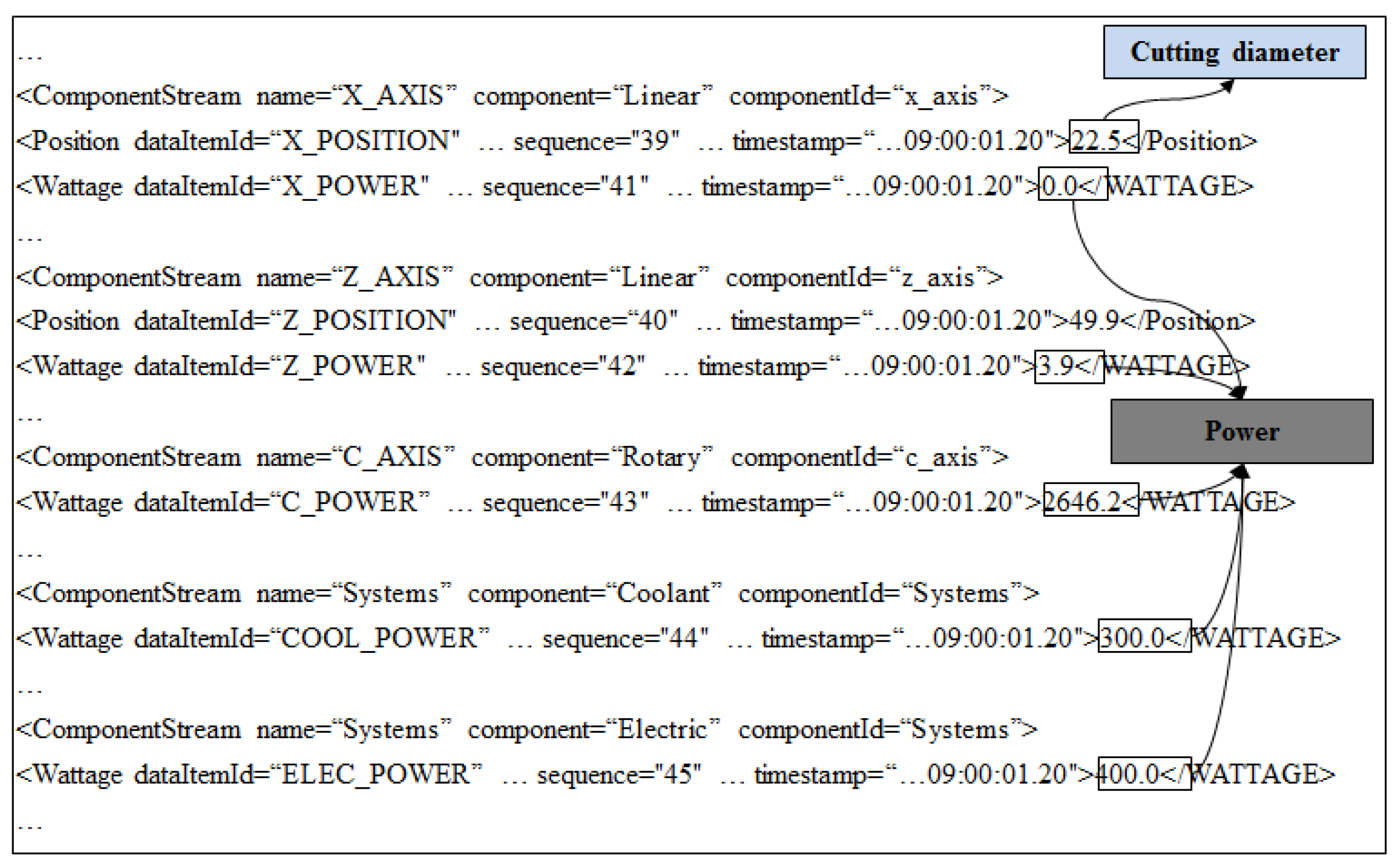
We choose MTConnect as the data interface for machine-monitoring data. The structure of MTConnect defines an information model in terms of the machine tool’s constituent axes, spindles, programs, and control sequences [2]. An MTConnect document includes: (1) a sample data item, which is the value of a continuous data stream at a point in time; (2) an event data item, which is an asynchronous change in state; and (3) a condition data item, which is the machine tool’s health and ability to function [40]. We can extract “cutting diameter” from each path position sample data item in the MTConnect document. We can extract “power consumption” from the summation of time-series wattage sample data items of machine tool components. Figure 5 shows an example of the PFD extraction from an MTConnect document.
2.2.2. Preparation of Training Datasets
When machine tools carry out actual machining, we can collect instances of PFD items through the extraction process described above. We then need to prepare training datasets by aggregating and fusing the instances of PFD items, which are used for computing numerical functions described later.
As shown in Figure 1, we first group the PFD instances aggregated during MCs 1 and 2 into an intermediate dataset because they both use the same classification data items except “path trajectory”. We then regroup this intermediate set into two separate datasets with respect to changes in “path trajectory”. By this grouping of the PFD instances, we can prepare separate training datasets for two different models that predict the power consumed during rapid or feed movement. We use the PFD instances aggregated during MC 3 to create another model because this configuration uses different “workpiece material” and “insert material” from those of MCs 1 and 2. The PFD instances in Figure 1 make four different predictive models in terms of the MCs determined.
Table 2 presents an example of a training dataset that corresponds to a predictive model applicable to the case of the feed movement in MCs 1 and 2. Here, Samples 1, 2, and 3 are examples of the data samples collected from MC 1. Samples 4 and 5 are examples of the data samples from MC 2. Even the same values of the input variables can make slightly different power values due to certain reasons such as machine’s chatter, insert’ wear, and tool holder’s misalignment. These five samples that are collected during machining two parts make one predictive model because their MCs (Machine 1, Turning tool, TiN-coated, Aluminum, Contouring rough, On, Feed) are set to be identical.
2.2.3. Computation of Numerical Functions
We can perform regression analysis to compute numerical functions by using training datasets described above. Several regression analysis techniques such as polynomial, nonlinear, and Bayesian linear regressions can be applicable to find statistically-significant relationships between the input data and the output data. Also, we can apply an Artificial Neural Network (ANN) technique for this purpose.
ANN is capable of learning from a dataset to describe nonlinear input-and-output relationships by characterizing topology, weight factors, bias and activation functions that are used in hidden and output layers of the network [41]. It is a commonly-used technique for pattern matching that recognizes patterns and matches inputs to those patterns in the areas such as speech and image recognition and classifier systems [42]. In the area of metal cutting, it is also commonly-used for predicting machining performances [43]. It has been effectively employed for supervised learning where the training is supervised and the desired outputs are also supplied during training [41]. Our problem is supervised learning because we identified the input and output variables necessary for creating predictive models. Moreover, ANN helps create a predictive model easily when a new MC appears because it just requires a new training dataset without any change of the structure of the networks. Even when existing MCs require recalculation of their models due to some reasons such as the calibration of data values, ANN can recalculate the models efficiently through adjusting weighting factors and bias.
Figure 6 presents the structure of the back propagation neural network consisting of input, hidden and output layers. Each MC has a numerical function computed by this neural network. Here, xi represents ith input. N and M represent each number of neurons in each hidden layer. A neuron is an information-processing unit that is fundamental to the operation of the neural network. wji, wkj, and wlk indicate the weight factors between the neurons of four layers. fh and fo are activation functions of the neurons from the hidden layer and output layer, respectively [42].
2.2.4. Performance Measurement of Numerical Functions
The computed functions require quantitative validation and measurement to assure their performances above a satisfactory threshold level. For example, we can validate the functions through the cross validation technique that partitions the data into training data to establish the functions and validation data to verify them. We can measure the accuracy of the functions through Root-Mean-Square Error (RMSE) analysis of the differences between predicted values and measured values.
Uncertainty Quantification (UQ) is important in predictive modeling, although this UQ is out-of-scope for this paper. Data uncertainty can occur due to sparse, imprecise, qualitative, subjective, faulty, or missing data. Also, model uncertainty can exist in the models [44]. The data and model uncertainty can decrease the model’s ability to predict results correctly. The UQ helps characterize the sources of the uncertainty and measure the probability distribution of the data and finally find some controllable solutions.
3. Analysis and Results
We demonstrate our modeling approach through a case study. Here, we obtain machine-monitoring data from the machining simulator that can generate MTConnect documents from the input of process plan data [45].
3.1. Case Scenario
Two turning machine tools manufacture a turned part, and they execute the batch production for each workpiece material. The workpiece has three types of metallic materials, including aluminum (AL), steel (STL), and titanium (TI). Each machine tool produces the parts which are weekly allocated: Machine 1 (700 parts: 300 AL parts, 150 STL parts, and 250 TI parts), and Machine 2 (350 parts: 150 AL, 150 STL, and 50 TI). Each machine tool has its unique capabilities, assuming Machine 1 is a more efficient machine tool than Machine 2 with respect to the machine power consumed during idle state and rapid movement.
A cylindrical workpiece passes through a machine tool to execute a contouring rough (termed in ISO 14649) machining operation to produce the same general revolution turning feature. The process parameters—feed rate, spindle speed, and cutting depth—control the contouring rough operation. Here, we assign the three process parameters randomly using a uniform distribution within the allowable ranges listed in Table 3. The ranges of the process are normally given by textbooks and handbooks [34]. This machining operation uses the same cutting tool (general turning tool), insert (TiN-coated), and coolant option (coolant on). In other words, this case study uses the same MC with respect to “cutting tool type”, “insert material”, “machining operation”, and “cooling type”. This process plan scenario generates a set of STEP-NC programs. Each set of STEP-NC programs is assigned to each machine tool to produce the allocated parts.
3.2. Creation of Predictive Models
Given the case scenario above, the machining simulator generates MTConnect documents that record the two machine tools’ movements [45]. An identical value set of the process parameters can result in slightly different power consumption due to randomized values to capture chatter (Machine 1: ±10% uniform-random deviation on cutting power, and ±5% uniform-random deviation on machine power; Machine 2: ±15% on cutting power, and ±10% on machine power). We prepare training datasets, as described in Section 2.2.2. Based on the training datasets, we create twelve predictive models for power consumption in terms of the combination of two machine tools, three workpiece materials, and two different path trajectories. In other words, the three MC data items—“machine tool model”, “workpiece material”, and “path trajectory”—have different combinations in the twelve models. Each model corresponds to each combination of a machine tool, a workpiece material, and a rapid or feed movement. To compute numerical functions of the twelve predictive models, we generate twelve Multi-layer Perceptron neural networks with one hundred maximum iterations, two hidden layers, five neurons with logistic activation functions per each hidden layer, one input layer, and one output layer. We use KNIME, a statistics and data mining tool, to generate these neural network models [46]. A neural network inputs a set of the input variables—feed rate (f), spindle speed (N), cutting depth (t), and cutting diameter (D)—and outputs the output variable, power consumption. For example, Table 4 shows weight factors and bias values given in neurons per layer in the case of a combination of “Machine 1”, “AL”, and “feed”. All the predictive models have this kind of neural network models.
3.3. Performance Analysis of Predictive Models
Using the machining simulator, we create validation datasets to analyze the performances of the created predictive models. We newly generate these validation datasets from another weekly allocation (numbers of validation data samples appear in Table 5). Due to the random assignment of process parameters, the weekly allocation with differing STEP-NC programs results in validation datasets different from the training datasets used in the creation of the twelve predictive models before. Also, the random deviation on the cutting and machine power makes different measured values even in the same set of the process parameters. The performance analysis of the models is described below:
- (1)
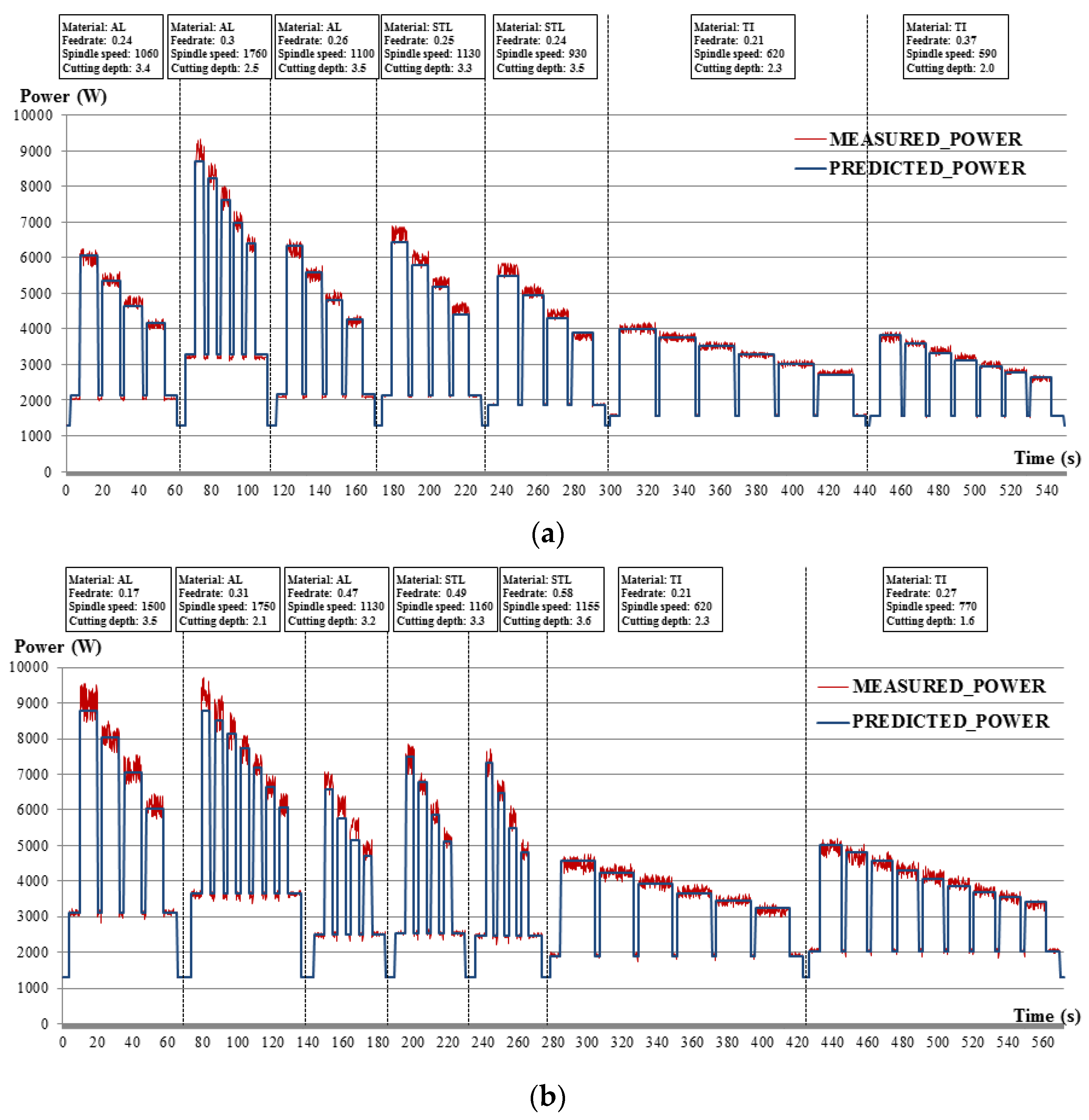
- Comparison between the measured power and the predicted power: Using the validation datasets, we can make a time-series of measured and predicted power profiles for the two machine tools’ operations. Figure 7 presents some captures of the power profiles to compare the predicted power that the predictive models generate with the measured power that the machining simulator generates. Figure 7a,b show the power profiles of Machine 1 and Machine 2, respectively, which produce seven parts with three workpiece materials and different process parameter sets. The predicted power coincides well with the measured power. The cutting power and the machine power have separate patterns on the measured power. The cutting power varies in terms of the values of feed rate, spindle speed, and cutting depth. Also, it gradually decreases as cutting diameter decreases. The machine power keeps steady state during spindle rotation. Our predictive models can capture these phenomena.
- (2)
- Statistical analysis of predictive models: we perform statistical analysis for the twelve predictive models computed by neural networks using statistical metrics including the coefficient of determination (R2) and the RMSE. Table 5 shows the result. The values of the statistical metrics indicate our predictive models can make good performances with minimum 84.1% R2 and maximum 0.066 RMSE. It is noted that the RMSE is measured on a 0-to-1 scale for min-max normalization of power values.
- (3)
- Power distributions in predictive models: We analyze the power distribution of each predictive model to check its accuracy to predict the desired results correctly within the range of minimum and maximum power. Figure 8a presents, for example, the scatter plot that maps the normalized predicted power with the normalized measured power for the case of “Machine 1”,“TI”, and “feed”. Here, the normalized power means a 0-to-1 scaled power converted from an original power value. The accuracy of the predictive model coincides with the middle of the power distribution. However, it falls off at both edges of the power distribution. In particular, these models slightly lose their predictive power at the top area of power distribution. The predicted power is distributed from 0.079 to 0.828; whereas, the measured power is distributed from 0 to 1. The RMSEs, respectively, score 0.022 in the validation samples less than the first quartile number, 0.021 in the samples between the first quartile and the third quartile numbers. However, the RMSE indicates 0.035 in the samples higher than the third quartile number. This fall-off occurs in all the predictive models. We conjecture that the distribution of the training dataset is left-skewed, as shown in Figure 8b; and thus the number of training data samples for predicting higher power values is very small compared to the numbers for lower and middle power values to learn these data samples.
4. Discussion
Case study demonstrates the feasibility and effectiveness of the proposed approach, which uses predictive models that are generated from the machining data. The proposed approach can be efficient for creating multiple predictive models that reflect the diversity of MCs (see Section 3.3 (1)). Also, it can make fine-grained models predictable up to the level of an NC program (see Section 3.3 (1)). These created models show good accuracy to predict power consumption (see Section 3.3 (2)).
We find a practical issue related to the application of the proposed approach. Though the predictive models computed by the neural network produce good results, the results are not good at very high power values (see Section 3.3 (3)). The distributions of the three process parameters were too narrow to represent the accuracy consistently across the entire ranges of observed process parameters. We need to broaden the ranges of values of the process parameters to sustain the accuracy and decrease the learning bias. For example, we can broaden the ranges of feed rate in Table 3, and then obtain their associating training datasets for sustaining the accuracy within the desired ranges.
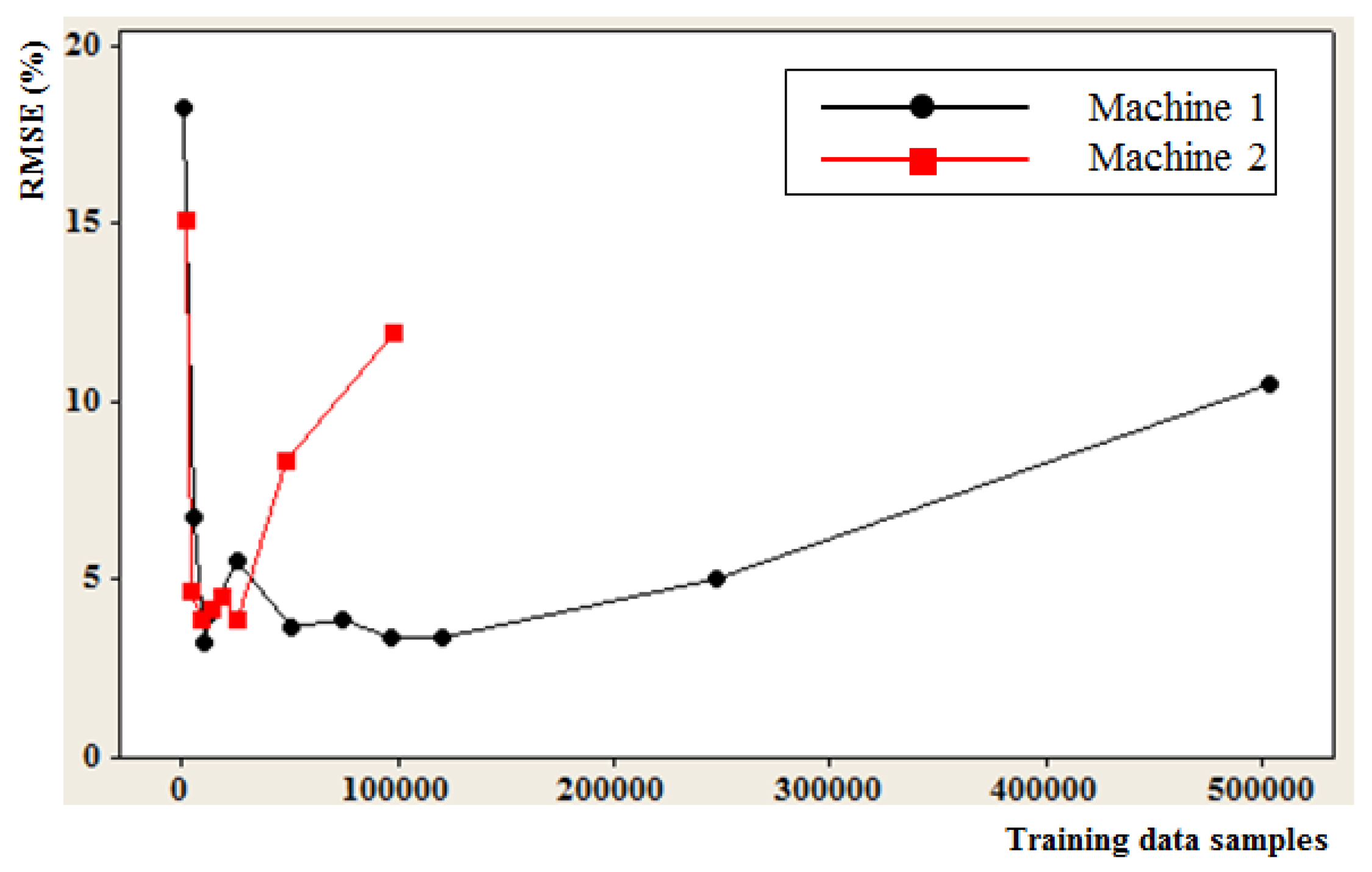
Another practical issue is the determination of the number of training data samples. There is no rigid rule for determining the number of training samples for power prediction using neural networks. Thus, we need to analyze the dependency between the number of training samples and statistical results for determining that number. We measure the change of the RMSE with regard to the increase of the number of training data samples. Figure 9 shows the trend graph that plots the numbers of training data samples and their corresponding RMSEs for the case of the TI material and two machine tools. As the sample sizes increase and the under-fitting of the ANN-based models decreases, RMSEs decrease to below 5% by about 6000 samples for Machine 1 and by 3000 samples for Machine 2. On the other hand, the ANN-based models start to increase the RMSEs when they, respectively, reach about 250,000 training samples in Machine 1 and about 50,000 training samples in Turning 2. This phenomenon is due to the over-fitting problem, which undermines a generalization ability of ANN-based models and can be caused from larger training data sizes than needed to solve the given problem [47].
5. Conclusions
This paper presented a standard data-based modeling approach to predict power consumption in turning machining operations. For this purpose, we described how to identify and categorize the MC, input, and output data among machining data, and then how to create predictive models using the identified and categorized data. The methodology presented in this paper can provide a good ability of prediction for process planning decisions on the basis of historical data collected from machining operations. The methodology allows manufacturers to create multiple predictive models that can be applied to diverse MCs. The methodology enables manufacturers to create fine-grained models predictable up to the level of an NC program. The methodology uses standardized data interfaces such as STEP-NC and MTConnect to provide comprehensiveness and interoperability to capture and share the machining data.
A machining shop can benefit from the application of hundreds or thousands of instances of predictive models for its machining facilities and operations. To provide these multiple instances of predictive models, we are developing a logically-organized framework that can design and operate these predictive models. This framework reduces the number of times of running the predictive modeling process by clustering together some MCs where the similarity in the relationships between input and output variables is found. This framework also constructs a common pool that accumulates predictive models to be used as building blocks. It enables common, reusable, and extensible applications of predictive models across machining shops. This is a significant advantage over traditional modeling approaches based on regression models. This is another reason why we use standardized data interfaces that can provide an open data sharing environment across machining shops.
As we mentioned in Section 1, data collecting is an important process because our approach uses historical machining data. A machining shop accumulates a large volume of machine-monitoring data as the number and the operation time of machine tools increase. A conventional database environment cannot efficiently manage the large volume of the data needed to perform fast retrieval and processing for runtime decision-making. Thus, it is helpful to use distributed database techniques such as Hadoop Distributed File System and its associated programming techniques such as MapReduce. We are currently developing this data infrastructure to increase the abilities of data retrieval and processing across machining shops.
Some limitations of this paper were the use of machine-monitoring data generated from a machining simulator, and the inability of predictive models to sustain high accuracy in high power values. Also, UQ was the out-of-scope of this paper. Future works include: (1) using real data collected from actual machining operations; (2) establishing consistency of high accuracy across full ranges of power values; and (3) integrating methodologies of UQ.
Acknowledgments
This research was supported by the National Research Foundation of Korea (NRF) grant funded by the Korea government (MSIP) (No. NRF-2016R1C1B1008820).
Author Contributions
All authors conceived the research idea and the methods of this study. Seung-Jun Shin and Jungyub Woo conceived and designed the experiments; Sudarsan Rachuri contributed modeling processes; Prita Meilanitasari analyzed the data in simulation; Seung-Jun Shin, Jungyub Woo, and Sudarsan Rachuri wrote the paper.
Conflicts of Interest
The authors declare no conflict of interest.
References
- Shin, S.J.; Suh, S.H.; Stroud, I. A green productivity based process planning system for a machining process. Int. J. Prod. Res. 2014, 53, 5085–5105. [Google Scholar] [CrossRef]
- Vijayaraghavan, A.; Dornfeld, D. Automated energy monitoring of machine tools. CIRP Ann. Manuf. Technol. 2010, 59, 21–24. [Google Scholar] [CrossRef]
- Gutowski, T.; Dahmus, J.; Thiriez, A. Electrical energy requirements for manufacturing processes. In Proceedings of the 13th CIRP International Conference on Life Cycle Engineering, Leuven, Belgium, 31 May–2 June 2006; pp. 623–628. [Google Scholar]
- Kara, S.; Li, W. Unit process energy consumption models for material removal processes. CIRP Ann. Manuf. Technol. 2011, 60, 37–40. [Google Scholar] [CrossRef]
- Newman, S.T.; Nssehi, A.; Imani-Asrai, R.; Dhokia, V. Energy efficient process planning for CNC machining. CIRP J. Manuf. Sci. Technol. 2012, 5, 127–136. [Google Scholar] [CrossRef] [Green Version]
- Altintas, Y. Manufacturing Automation: Metal Cutting Mechanics, Machine Tool Vibrations, and CNC Design; Cambridge University Press: New York, NY, USA, 2011. [Google Scholar]
- Bayoumi, A.E.; Yucesan, G.; Hutton, D.V. On the closed form mechanistic modeling of milling: Specific cutting energy, torque, and power. Mater. Eng. Perform. 1994, 3, 151–158. [Google Scholar] [CrossRef]
- Munoz, A.A.; Sheng, P. An analytical approach for determining the environmental impact of machining processes. Mater. Process. Technol. 1995, 53, 736–758. [Google Scholar] [CrossRef]
- Kishawy, H.A.; Kannan, S.; Balazinski, M. An energy based analytical force model for orthogonal cutting of metal matrix composites. CIRP Ann. Manuf. Technol. 2004, 53, 91–94. [Google Scholar] [CrossRef]
- Palanisamy, P.; Rajendran, I.; Shanmugasundaram, S.; Saravanan, R. Prediction of cutting force and temperature rise in the end-milling operation. Proc. Inst. Mech. Eng. Part B J. Eng. Manuf. 2006, 220, 1577–1587. [Google Scholar] [CrossRef]
- Astakhov, V.P.; Xiao, X. The principle of minimum strain energy to fracture of the workpiece material and its application in modern cutting technologies. In Metal Cutting Technology; Davim, J.P., Ed.; Walter de Gruyter GmbH & Co.: Berlin, Germany, 2016. [Google Scholar]
- Dietmair, A.; Verl, A. Energy consumption forecasting and optimization for tool machines. Mod. Mach. Sci. J. 2009, 62–67. [Google Scholar] [CrossRef]
- Weinert, N.; Chiotellis, S.; Seliger, G. Methodology for planning and operating energy-efficient production systems. CIRP Ann. Manuf. Technol. 2011, 60, 41–44. [Google Scholar] [CrossRef]
- Draganescu, F.; Gheorghe, M.; Doicin, C.V. Models of machine tool efficiency and specific consumed energy. Mater. Process. Technol. 2003, 141, 9–15. [Google Scholar] [CrossRef]
- Diaz, N.; Ninomiya, K.; Noble, J.; Dornfeld, D. Environmental impact characterization of milling and implications for potential energy savings in industry. Procedia CIRP 2012, 1, 518–523. [Google Scholar] [CrossRef]
- Astakhov, V.P.; Xiao, X. A methodology for practical cutting force evaluation based on the energy spent in the cutting system. Mach. Sci. Technol. 2008, 12, 325–347. [Google Scholar] [CrossRef]
- Helu, M.; Rühl, J.; Dornfeld, D.; Werner, P.; Lanza, G. Evaluating trade-offs between sustainability, performance, and cost of green machining technologies. In Proceedings of the 18th CIRP International Conference on Life Cycle Engineering, Braunschweig, Germany, 2–4 May 2011; pp. 195–200. [Google Scholar]
- Iqbal, A.; Zhang, H.C.; Kong, L.L.; Hussain, G. A rule-based system for trade-off among energy consumption, tool life, and productivity in machining process. J. Intell. Manuf. 2015, 26, 1217–1232. [Google Scholar] [CrossRef]
- Peng, T.; Xu, X. A holistic approach to achieving energy efficiency for interoperable machining systems. Int. J. Sustain. Eng. 2013, 7, 111–129. [Google Scholar] [CrossRef]
- Jia, S.; Tang, R.; Lv, J. Therblig-based energy demand modeling methodology of machining process to support intelligent manufacturing. J. Intell. Manuf. 2014, 25, 913–931. [Google Scholar] [CrossRef]
- Bhinge, R.; Biswas, N.; Dornfeld, D.; Park, J.K.; Law, K.; Helu, M.; Rachuri, S. An intelligent machine monitoring system for energy prediction using a Gaussian process regression. In Proceedings of the 2014 IEEE International Conference on Big Data, Washington, DC, USA, 27–30 October 2014; pp. 978–986. [Google Scholar]
- Behrendt, T.; Zein, A.; Min, S.K. Development of an energy consumption monitoring procedure for machine tools. CIRP Ann. Manuf. Technol. 2012, 61, 43–46. [Google Scholar] [CrossRef]
- Campatelli, G.; Lorenzini, L.; Scippa, A. Optimization of process parameters using a response surface method for minimizing power consumption in the milling of carbon steel. J. Clean. Prod. 2014, 66, 309–316. [Google Scholar] [CrossRef]
- International Standards Organization (ISO). ISO14649. Industrial Automation Systems and Integration—Physical Device Control—Data Model for Computerized Numerical Controllers—Part 1: Overview and Fundamental Principles; International Standards Organization: Geneva, Switzerland, 2003. [Google Scholar]
- MTConnect. MTConnect Standard Part 1—Overview and Protocol; MTConnect Institute: McLean, VA, USA, 2011. [Google Scholar]
- Mori, M.; Fujishima, M.; Inamasu, Y.; Oda, Y. A study on energy efficiency improvement for machine tools. CIRP Ann. Manuf. Technol. 2011, 60, 145–148. [Google Scholar] [CrossRef]
- Aramcharoen, A.; Mativenga, P.T. Critical factors in energy demand modelling for CNC milling and impact of toolpath strategy. J. Clean. Prod. 2014, 78, 63–74. [Google Scholar] [CrossRef]
- Abushawashi, Y.; Xiao, X.; Astakhov, V. A novel approach for determining material constitutive parameters for a wide range of triaxiality under plane strain loading conditions. Int. J. Mech. Sci. 2013, 74, 133–142. [Google Scholar] [CrossRef]
- Astakhov, V.P.; Shvets, S. The assessment of plastic deformation in metal cutting. J. Mater. Process. Technol. 2004, 146, 193–202. [Google Scholar] [CrossRef]
- Li, J.; Lu, Y.; Zhao, H.; Li, P.; Yao, X. Optimization of cutting parameters for energy saving. Int. J. Adv. Manuf. Technol. 2014, 70, 117–124. [Google Scholar] [CrossRef]
- Zhang, Y.; Zou, P.; Li, B.; Liang, S. Study on optimized principles of process parameters for environmentally friendly machining austenitic stainless steel with high efficiency and little energy consumption. Int. J. Adv. Manuf. Technol. 2015, 79, 89–99. [Google Scholar] [CrossRef]
- Shokrani, A.; Dhokia, A.; Newman, S.T. Environmentally conscious machining of difficult-to-machine materials with regard to cutting fluids. Int. J. Mach. Tools Manuf. 2012, 57, 83–101. [Google Scholar] [CrossRef] [Green Version]
- Velchev, S.; Kolev, I.; Ivanov, K.; Gechevski, S. Empirical models for specific energy consumption and optimization of cutting parameters for minimizing energy consumption during turning. J. Clean. Prod. 2014, 80, 139–149. [Google Scholar] [CrossRef]
- Amstead, B.H.; Ostwald, P.F.; Begeman, M. Manufacturing Processes; John Wiley & Sons Inc.: New York, NY, USA, 1987. [Google Scholar]
- Bhushan, R.K. Optimization of cutting parameters for minimizing power consumption and maximizing tool life during machining of Al alloy SiC particle composites. J. Clean. Prod. 2013, 39, 242–254. [Google Scholar] [CrossRef]
- International Standards Organization (ISO). ISO/TS14649. Industrial Automation Systems and Integration—Physical Device Control—Data Model for Computerized Numerical Controllers—Part 201: Machine Tool Data for Cutting Processes; International Standards Organization: Geneva, Switzerland, 2011. [Google Scholar]
- International Standards Organization (ISO). ISO14649. Industrial Automation Systems and Integration—Physical Device Control—Data Model for Computerized Numerical Controllers—Part 12: Process Data for Turning; International Standards Organization: Geneva, Switzerland, 2005. [Google Scholar]
- International Standards Organization (ISO). ISO14649. Industrial Automation Systems and Integration—Physical Device Control—Data Model for Computerized Numerical Controllers—Part 121: Tools for Turning Machines; International Standards Organization: Geneva, Switzerland, 2005. [Google Scholar]
- International Standards Organization (ISO). ISO 6983. Automation Systems and Integration—Numerical Control of Machines—Program Format and Definitions of Address Words—Part 1: Data Format for Positioning, Line Motion and Contouring Control Systems; International Standards Organization: Geneva, Switzerland, 2009. [Google Scholar]
- MTConnect. MTConnect Standard Part 2—Components and Data Items; MTConnect Institute: McLean, VA, USA, 2012. [Google Scholar]
- Chandrasekaran, M.; Muralidhar, M.; Krishna, C.M.; Dixit, U.S. Application of soft computing techniques in machining performance prediction and optimization: A literature review. Int. J. Adv. Manuf. Technol. 2010, 46, 445–464. [Google Scholar] [CrossRef]
- Lippmann, R.P. An introduction to computing with neural nets. IEEE ASSP Mag. 1987, 4, 4–22. [Google Scholar] [CrossRef]
- Szecsi, T. Cutting force modeling using artificial neural networks. J. Mater. Process. Technol. 1999, 92, 344–349. [Google Scholar] [CrossRef]
- Nannapaneni, S.; Mahadevan, S. Uncertainty quantification in performance evaluation of manufacturing processes. In Proceedings of the 2014 IEEE International Conference on Big Data, Washington, DC, USA, 27–30 October 2014; pp. 996–1005. [Google Scholar]
- Shin, S.J.; Woo, J.W.; Kim, D.B.; Kumaraguru, S.; Rachuri, S. Developing a virtual machining model to generate MTConnect machine-monitoring data from STEP-NC. Int. J. Prod. Res. 2015, 54, 4487–4505. [Google Scholar] [CrossRef]
- KNIME Analytics Platform. Available online: http://www.knime.org/ (accessed on 29 July 2014).
- Markopoulos, A.P.; Manolakos, D.E.; Vaxevanidis, N.M. Artificial neural network models for the prediction of surface roughness in electrical discharge machining. J. Intell. Manuf. 2008, 19, 283–292. [Google Scholar] [CrossRef]
Figure 1.
A time-series power profile and machining configurations on a machine tool.
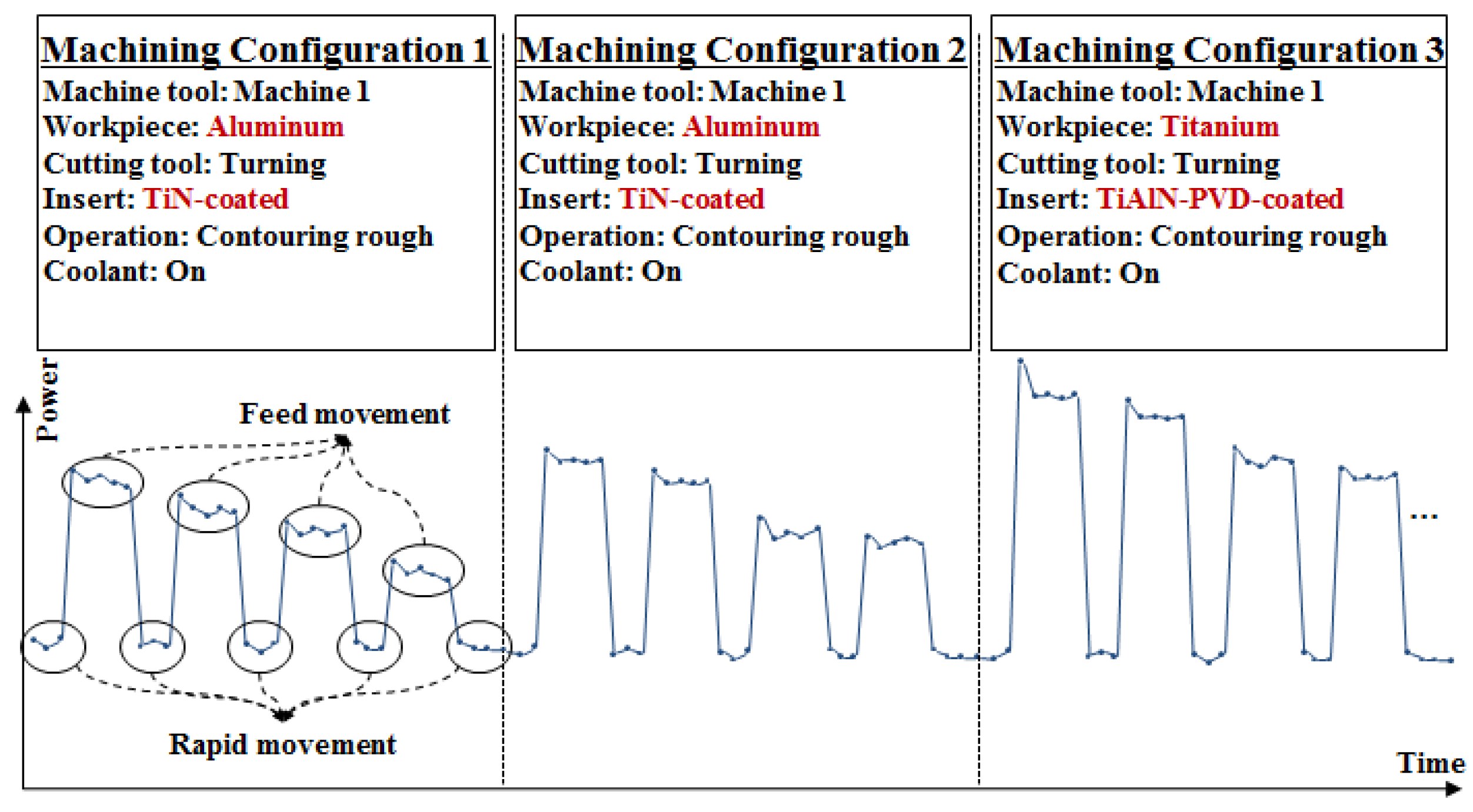
Figure 2.
A structure for relations of machining configurations and their model components.
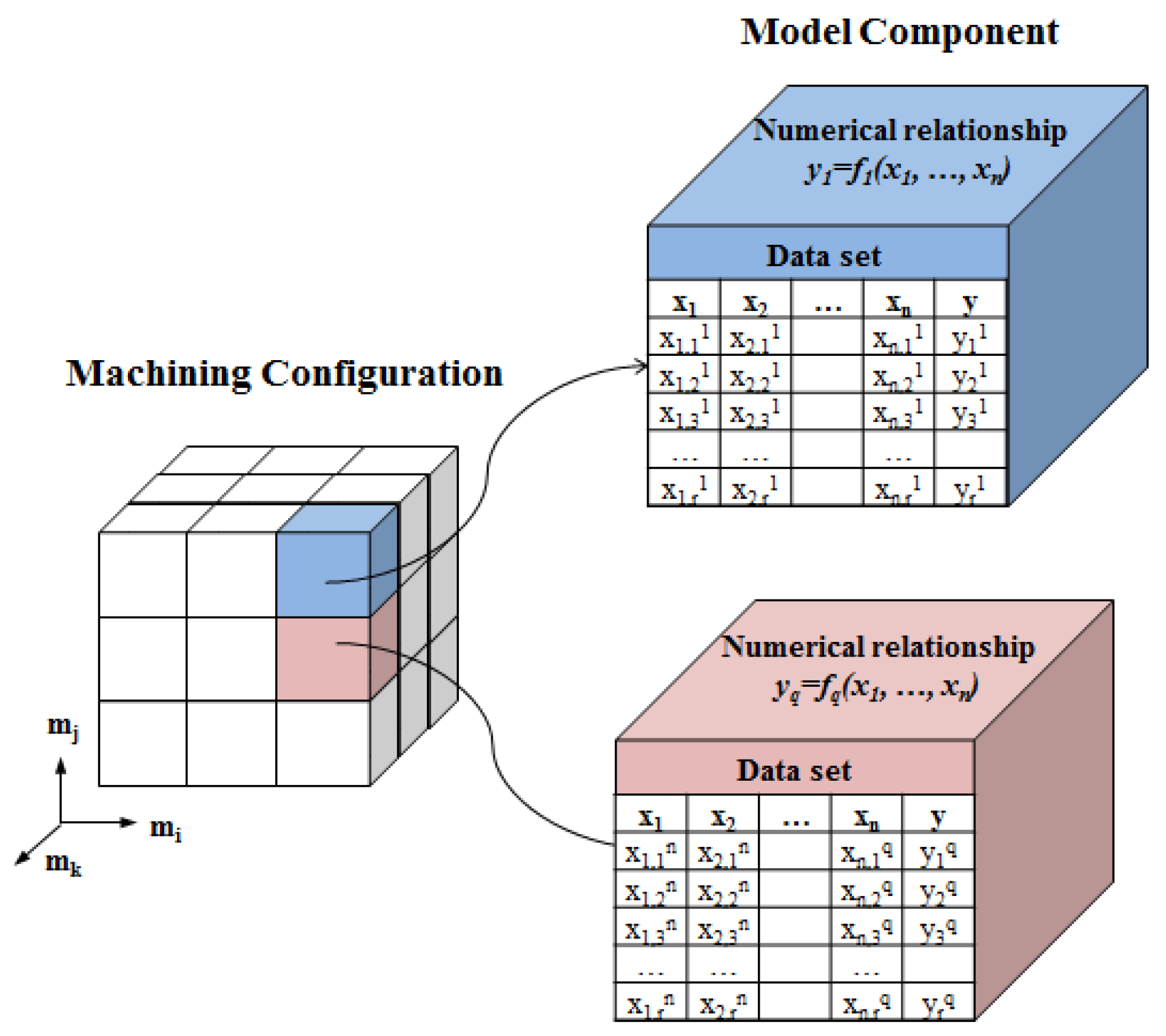
Figure 3.
An example of PFD extraction from a STEP-NC program.
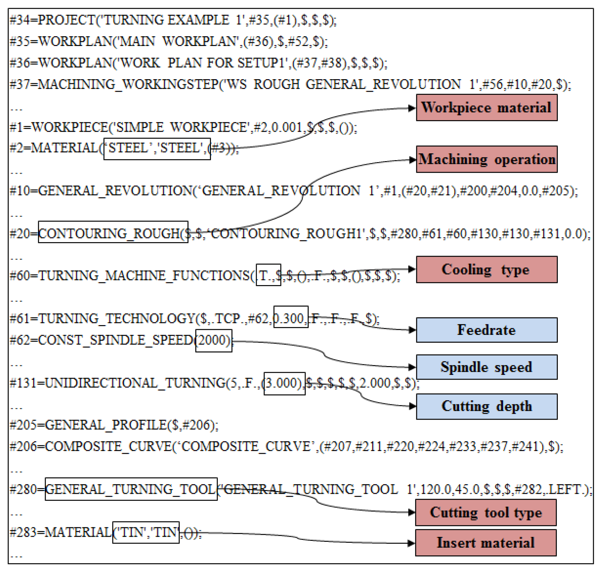
Figure 4.
An example of PFD extraction from a Numerical Control program.
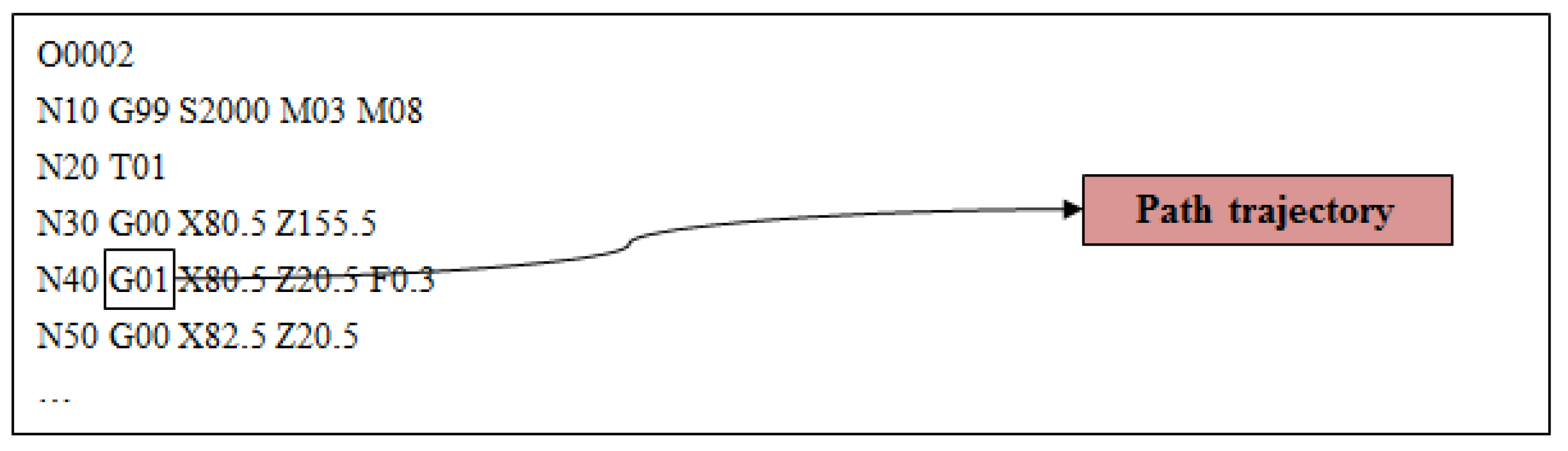
Figure 5.
An example of PFD extraction from an MTConnect document.

Figure 6.
A structure of a neural network on a machining configuration.
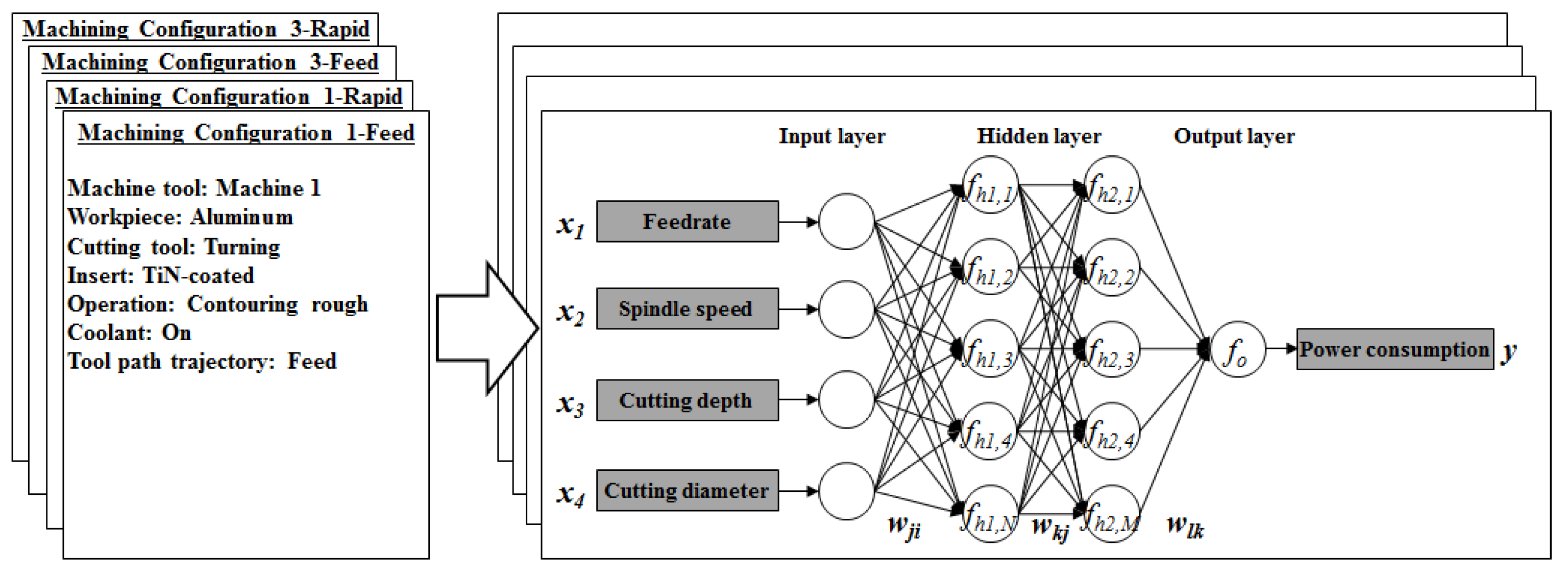
Figure 7.
A comparison between the measured power and predicted power. (a) Power profiles on Machine 1; (b) Power profiles on Machine 2.
Figure 7.
A comparison between the measured power and predicted power. (a) Power profiles on Machine 1; (b) Power profiles on Machine 2.

Figure 8.
Power distribution and training data sample distribution (“Machine 1”, “TI”, “feed”). (a) A scatter plot of measured power and predicted power; (b) A distribution of training data samples.
Figure 8.
Power distribution and training data sample distribution (“Machine 1”, “TI”, “feed”). (a) A scatter plot of measured power and predicted power; (b) A distribution of training data samples.
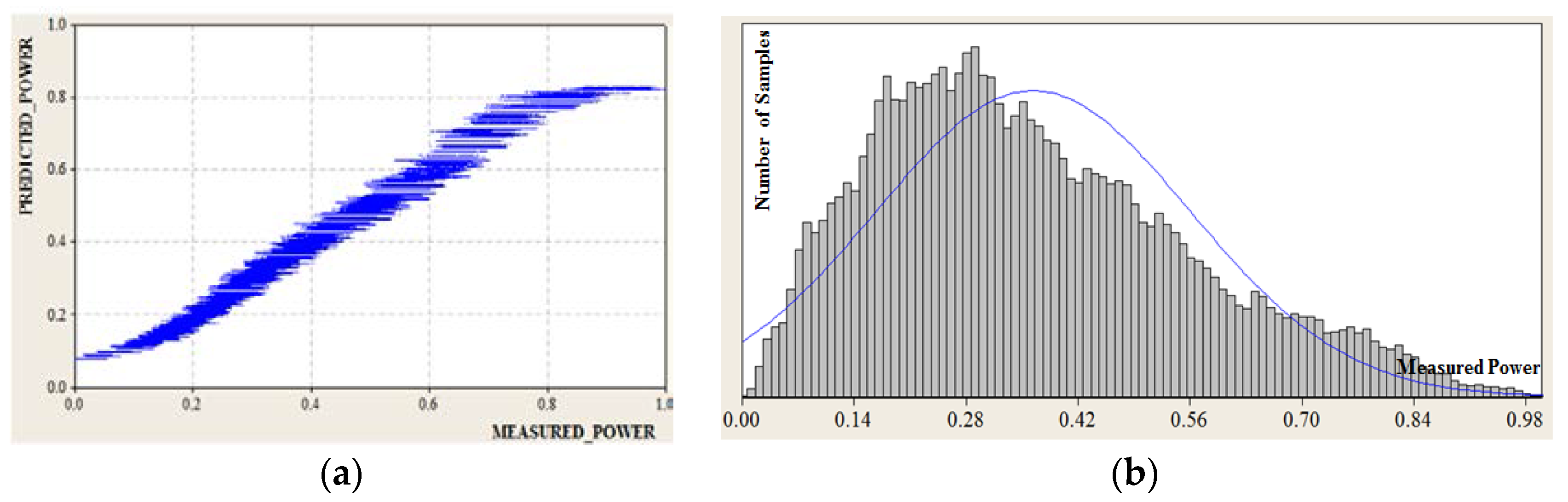
Figure 9.
A trend graph of RMSE with regard to increase of training data samples.

Table 1.
A list of Process Feature Data (PFD) items.
| Category | PFD Item | Influencing Variable | Data Type | Examples |
|---|---|---|---|---|
| Machining configuration | Machine tool model | Pmachine | Nominal | Machine tool 1, Machine tool 2 |
| Cutting tool type | k | Nominal | Turning, Grooving, End mill | |
| Insert material | k | Nominal | Titanium coated, High speed steel | |
| Workpiece material | k | Nominal | Aluminum, Steel, Titanium | |
| Machining operation | k | Nominal | Contouring, Facing, Rough or Finish | |
| Cooling type | k | Nominal | Emulsion, Mineral Oil, Dry | |
| Path trajectory | k | Enumeration | Rapid/Feed | |
| Input variable | Cutting depth | Q | Numeric | |
| Feed rate | Q | Numeric | ||
| Spindle speed | Q | Numeric | ||
| Cutting diameter | Q | Numeric | ||
| Output variable | Power consumption | P | Numeric |
Table 2.
An example of a training dataset.
| Machining Configuration Number | Sample No. | Input Variables | Output Variable | |||
|---|---|---|---|---|---|---|
| Cutting Depth | Feed Rate | Spindle Speed | Cutting Diameter | Power Consumption | ||
| 1 | 1 | 1.6 | 0.27 | 1000 | 23.4 | 4598.3 |
| 2 | 1.6 | 0.27 | 1000 | 23.4 | 4561.1 | |
| 3 | 1.6 | 0.27 | 1000 | 21.8 | 4343.1 | |
| ... | ||||||
| 2 | 4 | 2.8 | 0.46 | 1137 | 22.2 | 6294.3 |
| 5 | 2.8 | 0.46 | 1137 | 19.4 | 5554.5 | |
| … | ||||||
Table 3.
Range of process parameters.
| Process Parameter | Unit | Workpiece Material | ||
|---|---|---|---|---|
| AL | STL | TI | ||
| Feed rate | mm/rev | 0.1–0.5 | 0.2–0.6 | 0.2–0.4 |
| Spindle speed | RPM | 900–2000 | 900–1200 | 500–1000 |
| Cutting depth | mm | 1–4 | 2–6 | 1–3 |
Table 4.
Weight factors and bias values (“Machine 1”, “AL”, “feed”).
| Hidden Layer 1 | Hidden Layer 2 | Output Layer | ||||||||||||||
|---|---|---|---|---|---|---|---|---|---|---|---|---|---|---|---|---|
| Neuron | N1,0 | N1,1 | N1,2 | N1,3 | N1,4 | Neuron | N2,0 | N2,1 | N2,2 | N2,3 | N2,4 | Neuron | N3,0 | |||
| Input | Input | Input | ||||||||||||||
| f | −0.014 | 0.051 | 0.092 | −0.330 | −0.377 | N1,0 | 1.380 | 0.787 | 0.191 | 0.522 | −1.074 | N2,0 | −0.948 | |||
| N | −0.905 | 3.751 | 1.635 | 1.016 | −2.855 | N1,1 | 0.029 | −2.017 | −0.787 | 0.664 | 0.401 | N2,1 | −1.117 | |||
| t | −0.919 | 0.189 | 1.767 | 3.213 | 0.734 | N1,2 | −0.493 | −0.738 | −0.703 | 1.313 | 0.829 | N2,2 | −1.386 | |||
| D | −0.138 | −0.358 | 2.511 | 3.326 | 0.325 | N1,3 | −2.266 | −0.967 | −2.134 | 2.800 | 1.283 | N2,3 | 0.504 | |||
| Bias | 0.035 | −1.650 | −1.839 | −4.475 | 0.017 | N1,4 | −0.277 | 2.651 | 1.689 | 1.802 | −1.348 | N2,4 | 1.804 | |||
| Bias | −0.145 | 1.296 | 1.253 | −0.200 | 0.216 | Bias | −0.639 | |||||||||
Table 5.
Statistical analysis of the predictive models.
| Machine | Workpiece | Path Trajectory | Training Samples | Validation Samples | R2 (%) | RMSE |
|---|---|---|---|---|---|---|
| Machine 1 | AL | Feed | 77,241 | 74,683 | 96.7 | 0.031 |
| Rapid | 35,449 | 35,509 | 97.9 | 0.040 | ||
| STL | Feed | 16,679 | 16,217 | 95.9 | 0.044 | |
| Rapid | 12,944 | 12,879 | 97.1 | 0.042 | ||
| TI | Feed | 121,657 | 123,379 | 98.3 | 0.025 | |
| Rapid | 33,050 | 33,022 | 98.4 | 0.033 | ||
| Machine 2 | AL | Feed | 36,758 | 36,670 | 95.5 | 0.037 |
| Rapid | 20,657 | 20,615 | 98.2 | 0.033 | ||
| STL | Feed | 16,564 | 15,967 | 95.3 | 0.042 | |
| Rapid | 15,165 | 14,988 | 84.1 | 0.064 | ||
| TI | Feed | 25,684 | 22,329 | 96.8 | 0.035 | |
| Rapid | 8018 | 7740 | 88.1 | 0.066 |
© 2018 by the authors. Licensee MDPI, Basel, Switzerland. This article is an open access article distributed under the terms and conditions of the Creative Commons Attribution (CC BY) license (http://creativecommons.org/licenses/by/4.0/).
Share and Cite
MDPI and ACS Style
Shin, S.-J.; Woo, J.; Rachuri, S.; Meilanitasari, P. Standard Data-Based Predictive Modeling for Power Consumption in Turning Machining. Sustainability 2018, 10, 598. https://doi.org/10.3390/su10030598
AMA Style
Shin S-J, Woo J, Rachuri S, Meilanitasari P. Standard Data-Based Predictive Modeling for Power Consumption in Turning Machining. Sustainability. 2018; 10(3):598. https://doi.org/10.3390/su10030598
Chicago/Turabian StyleShin, Seung-Jun, Jungyub Woo, Sudarsan Rachuri, and Prita Meilanitasari. 2018. "Standard Data-Based Predictive Modeling for Power Consumption in Turning Machining" Sustainability 10, no. 3: 598. https://doi.org/10.3390/su10030598
Note that from the first issue of 2016, this journal uses article numbers instead of page numbers. See further details here.