Optimal Investment Planning of Bulk Energy Storage Systems

Abstract

Many countries have the ambition to increase the share of renewable sources in electricity generation. However, continuously varying renewable sources, such as wind power or solar energy, require that the power system can manage the variability and uncertainty of the power generation. One solution to increase flexibility of the system is to use various forms of energy storage, which can provide flexibility to the system at different time ranges and smooth the effect of variability of the renewable generation. In this paper, we investigate three questions connected to investment planning of energy storage systems. First, how the existing flexibility in the system will affect the need for energy storage investments. Second, how presence of energy storage will affect renewable generation expansion and affect electricity prices. Third, who should be responsible for energy storage investments planning. This paper proposes to assess these questions through two different mathematical models. The first model is designed for centralized investment planning and the second model deals with a decentralized investment approach where a single independent profit maximizing utility is responsible for energy storage investments. The models have been applied in various case studies with different generation mixes and flexibility levels. The results show that energy storage system is beneficial for power system operation. However, additional regulation should be considered to achieve optimal investment and allocation of energy storage.

1. Introduction

1.1. Motivation

The flexibility of a power system is defined by how well it can cope with variability and uncertainty and balance the production and consumption. Variability and uncertainty come from various sources such as time-varying demand and generation based on variable renewable sources as well as different contingencies such as line and generation outages.

Power systems are designed to handle demand variability and uncertainty as well as the majority of the contingencies. However, the increasing interest in variable renewable generation such as wind-based generation raises concerns on the need to increase the flexibility of the systems to accommodate large scale varying renewable energy sources. The capacity of wind energy installations is constantly increasing. For example, in Europe, the share of wind-based energy increased from 2.5 to 15.6% just over 15 years [1]. Current percentage of wind-based electricity generation in the European generation mix is now even greater than hydro based electricity generation which is 15.5%. Such a share of variable wind energy is still considered relatively low. In addition, the current state of a flexibility of the majority European power systems is proved to be sufficient to handle variability and uncertainty of the present wind based generation. However, if the trend will continue, power systems might have to improve the flexibility of the system. Based on current European targets, 20% consumption of energy should come from renewable generation by the year 2020. The target has been set by 2020 Climate and Energy package and will require even higher installed capacity of renewable generation due to variability and uncertainty of the renewable sources. Thus, wind power penetration is expected to grow substantially just over next few years. In addition, more ambitious targets are expected to be set for 2030 by Winter Package which is still under development. Increase in large scale renewable generation will contribute to higher volatility of wholesale electricity prices, higher balancing costs and system maintenance costs as well as large curtailments of renewable generation output. Thus, additional flexibility will be required [2,3].

The flexibility of the power system is provided mainly through flexible generation units with fast response time and flexible demand. One of the most flexible and least expensive generation units is hydro. The presence of hydropower in a power system clearly has a positive impact on the flexibility of the system. Hydrothermal power systems generally have good ramping capability and energy storage possibility in the form of hydro reservoirs. Thus, power system operators can use the flexibility of the hydropower generation to balance variable renewable electricity generation and load. However, for a large-scale expansion of wind power (or other variable generation such as solar) existing hydro flexibility might not be sufficient. More importantly, expansion of hydropower generation is difficult and in some cases is even impossible due to limited natural resources. In addition to hydropower, the flexibility of the system can then be improved by increasing the capacity of existing power plants, adding additional fast-ramping thermal generation capacity, demand response or energy storage capability. In this paper, we address the possibility to provide additional flexibility by adding energy storage capacity considering different storage technologies.

1.2. Knowledge Gap

Energy storage is not a new concept and was used for decades in power system, however predominantly pumped-hydro energy storage was in operation. Almost 99% of installed bulk energy storage capacity comes from pumped hydro and new installation of such energy storage is limited due to the same reasons as hydropower. However, other technologies such as compressed air energy storage (CAES) and various types of batteries are mature and available for applications on transmission level. In addition, other technologies for energy storage systems (ESS) are also under development and will be commercially available in foreseeable future. A database with a list of existing energy storage projects around the world is available in [4]. Energy storage systems are capable of providing additional flexibility on different time frames to power system operation by charging at peak hours and discharging when additional electricity is required. Such flexibility is very desirable for systems with high share of variable renewable generation. In addition, energy storage technologies are very fast and can be deployed at different capacities and power capabilities depending on the needs of the system. According to [5] the need in additional storage capacity in Europe alone is expected to double by 2050 mostly due to renewable generation capacity increase and additional balancing needs connected to that growth.

Energy storage systems (ESS) have multiple applications and can be beneficial at different levels of the electricity system. Various literature provide an overview on possible applications and assessment of energy storage benefits. In [6] a comprehensive analysis of possible energy storage applications and suitable energy storage technologies is presented. Applications may vary from energy arbitrage to grid upgrade investments deferral. The most promising applications for energy storage include energy arbitrage, balancing services and renewable generation support. Different ways how energy storage systems could be used for balancing applications, especially in presence of a large amount of variable renewable generation, were studied in [7,8], while [9] includes benefits of energy storage as a flexibility source. In addition, [10,11] analyze how energy storage can be beneficial for supporting variable wind power generation and [12] presents benefits of energy storage from a technical point of view and its effect on maximum wind power penetration. A review of modeling techniques of energy storage given different objectives is provided in [13] and includes more than 150 papers on the energy storage assessment subject. The literature provides evidence that energy storage is beneficial for renewable generation support and can be profitable under certain assumptions, however high capital cost is seen as the main obstacle in energy storage market development. Cost evaluation and calculation of different energy storage technologies is presented in [14,15].

The aforementioned papers have shown that additional capacity of flexibility sources such as energy storage will be required to reach future renewable targets and energy storage might be profitable in the systems with a high share of renewables but the financial profitability of the energy storage is still strongly dependent on the size and location of the deployed energy storage system. Optimal planning of energy storage under different conditions and objectives have been studied in [10,16,17,18,19,20,21,22]. In addition, [23,24,25,26,27] investigated joint optimal allocation and sizing of energy storage. In [28] the authors also show that energy storage is beneficial for renewable generation expansion and that joint optimization of renewable generation and flexibility sources including energy storage results in much higher cost savings than when investment planning is procured separately. However, these papers consider centralized investments planning which does not ensure profitability of the energy storage system itself and does not consider profit maximizing behaviour of the energy storage investor. Should flexibility sources such as energy storage be a market asset or system asset is an open question in power systems. Under current European regulation energy storage cannot be used to obtain profit if it is owned by system operators. Thus, current development of energy storage will mostly depend on independent investors which have profit maximizing objectives and other constraints on expected profit. A profit maximizing bilevel approach for investment planning of energy storage systems which will ensure that the owner of the energy storage will maximize its benefits has been proposed in [23,29,30]. However, neither of the proposed models include other sources of flexibility such as hydro and flexible demand which are currently the main competitors of emerging energy storage systems. Moreover, these models do not take into account possible growth of renewable generation.

1.3. Modeling Methodology

As in [23] this paper proposes a bilevel investment planning of strategic energy storage investor following the modeling approach proposed in [31] for generation investment planning. The approach allows to model behaviour of the strategic investor considering power system operation and locational marginal prices as an output of the operation. The modeling approach proposed in [31] allows to simulate operation of power system close to realistic operation and including many details such as dynamics of energy limited resources including energy storage, hydro power and flexible demand. Thus, the prices obtained to calculate energy storage profit are more realistic than using other mathematical models. In addition, the paper uses a technique to reformulate bilevel problem into single level linear program. Thus the obtained optimization problem can be solved with standard solvers such as CPLEX.

1.4. Contribution

This paper proposes two different mathematical models for joint energy storage sizing and allocation along with renewable generation expansion. The renewable generation expansion is ensured by expected renewable generation target constraint which sets the lower bound on renewable generation as a percentage of total consumption. The first model is for a centralized operation and investment planning while the second model is designed for an independent energy storage owner who is responsible for energy storage investments while the operation is still on a centralized planner. The proposed models can manage different generation sources (including thermal, hydro and variable renewable generation) along with flexible demand. The energy storage investment decisions are made over a portfolio of different energy storage technologies with varying properties for efficiency, self-discharge, etc. The owner of energy storage systems can decide which energy storage units to invest in and where to allocate them. The model has been applied to a case study under different cost parameters and various levels of installed flexibility. The proposed models and case study in this paper differ from the ones existing in the literature on four main points:

• First, the investment planning includes other sources of the flexibility of the system (hydro power and consumption flexibility) which can create competition for energy storage systems and affect the revenue stream.
• Second, energy storage investments are made along with renewable generation expansion and takes into account renewable generation targets present nowadays in Europe and USA.
• Third, the decentralized planning model in addition to investment return constraints includes payback period constraint which make the simulation of investment decision on energy storage closer to real life investment planning. Moreover, a solution to the bilevel problem has been suggested.
• Fourth, the paper presents a comparative analysis based on several case studies of systems with different generation mix and different levels of congestion. The results contribute to an understanding of the benefits of energy storage under different planning strategies and dependency of existing flexibility and type of flexibility on the profitability of the energy storage and possible effect on system congestion.

The models in this paper will be effective not only to help independent investment planning of energy storage owner considering expected growth of renewable generation but also to analyze the influence of existing flexibility in the system on energy storage investments.

1.5. Structure of the Paper

The paper is organized as follows. Section 2 introduces a centralized planning model followed by a bilevel mathematical formulation of a decentralized approach and a brief description of a one-level reformulation and linearization techniques. Section 3 presents case studies, results and an analysis of results. Finally, Section 4 provides conclusions and a discussion on a future work.

2. Energy Storage Investment Decision and Allocation Problem

The models in this paper consider two investment decisions: wind power generation expansion and energy storage investments. The first model (which is referred to as the centralized model) assumes perfect competition which could effectively be modeled by assuming that all operation and investment decisions are made by a single cost minimizing entity. The second model (which is referred to as the decentralized model) it is assumed that a separate entity makes decisions about energy storage investments, while the rest of the system remains a perfectly competitive market environment. The model assumes that the energy storage investor is a leader while the centralized planner is a follower meaning that first the decision on energy storage is made and afterwards based on that decision the centralized planner can expand renewable generation capacity and decide on operation dispatch. Thus, the energy storage entity can benefit from taking decision beforehand and strategically place energy storage while the centralized player can react to the investments and update its renewable generation capacity based on new flexibility in the system.

Both of the approaches have to take into account power system operation decisions, however the objectives are different. Thus, two different mathematical models were created in order to address the energy storage investment decision problem from two different ownership prospective. The following assumptions on energy storage investment decisions are taken for both models:

• The energy storage investor can choose between energy storage modules of different technologies, where each module has fixed energy capacity, power capability and other technical parameters such as self-discharge and efficiency.
• The energy storage charge and discharge efficiency as well as the self-discharge rate are fixed parameters and do not vary based on the charge/discharge output level or the energy level of the storage.

Additional assumptions are taken for each player.

• The centralized player is responsible for generation expansion investments into renewable energy.
• An independent investor will only make investments which will reach break-even within a given time. For example, typical expected payback period in long term investment planning is five years.
• An independent investor has a lower limit on minimum investments returns.
• The financial benefit of the energy storage is obtained through energy arbitrage.
• The energy storage utility can exchange information with the centralized player which is in charge of the optimal dispatch of the generation, flexible load and energy storage in the system. The centralized player receives information from energy storage owner about invested and available energy storage energy capacity and power capability of each unit. On the other hand the centralized player provides information about dispatch of each energy storage unit and electricity prices.
• The power system is represented by a DC load flow model.

2.1. Centralized Energy Storage Investment Decision and Allocation Problem

The investment decision problem for a centralized player is described in this section. The centralized player is responsible for the short-term operation of the power system and for the decisions on renewable generation expansion and investments and allocation of energy storage units. The problem is formulated as a mixed integer linear problem. Integer variables are used to allocate energy storage units while wind power generation investments are assumed to be continuous variables.

The objective function is described through Equation (1) and reflects the cost minimization of the whole system. The total cost consists of three main parts. The objective function is to minimize the cost of the scheduled day ahead generation dispatch $A_{p,s}$ based on the marginal generation cost of thermal units $m{c}_j$, energy storage charge and discharge cost $m{c}_e$ and charges to activate flexible load $\Delta d_d$. The marginal cost of the energy storage charging or discharging is usually equal to zero (except for compressed air energy storage which uses natural gas or fuel in the discharging process). However, to take into account fast degradation connected to the cycling of some energy storage technologies such as batteries, an additional variable cost is assigned to each charge and discharge. In order to evaluate operation of energy limited resources with storage capability we also consider future value of stored energy in hydro reservoirs and energy storage systems calculated in $B_{k,t,s}$. $F{C}_k$ is expected future price of electricity at the end of each operational period k. In addition to the variable costs, the system operator also minimize the investment cost into generation expansion and energy storage $C_t$. In this model we do not simulate all hours of operation of power system. Instead, we use selected days (for example number of seasons k = 4, number of selected days d = 1 and number of operation periods of each day l = 24 h). Thus, in order to match the simulated short-term operation costs of each year with and investment costs we use scale factor $\psi$ which can be calculated through simple formula ${\displaystyle \frac{8760}{k*l*d}}$ (for the given example it will be equal to 91.25).

$$\underset{{\Omega }_s}{Minimize:}{f}_{LL}=\sum _t(\psi \sum _s{\pi }_s(\sum _{k,l}{A}_{p,s}-\sum _k{B}_{k,t,s})+C_t)$$

(1)

where:

$$A_{p,s}=\sum _{j}m{c}_j{g}_{j,p,s}+\sum _{d}m{c}_d(\uparrow \Delta d_{d,p,s}+\downarrow \Delta d_{d,p,s})+\sum _{e}m{c}_e(g_{e,p,s}^{ch}+g_{e,p,s}^{dch})$$

(2)

$$B_{k,t,s}=F{C}_{k,t}(\sum _{e}SO{C}_{e,t,k,L,s}+\sum _h{\sigma }_h{v}_{h,t,k,L,s})$$

(3)

$$C_t=\sum _w{C}_{w,t}(G_{w,t}^{max}-G_{w,t-1}^{max})+\sum _e{C}_{e,t}(y_{e,t}-y_{e,t-1})$$

(4)

The minimization problem is a subject to various constraints.

Energy storage investment constraint (5) ensures that invested energy storage unit is available at the later time periods after the investment was made.

$$y_{e,t}\ge y_{e,t-1}\forall e,t$$

(5)

Equation (6) represents the power balance for each node of the system. Total generation and net injection should be equal to the total demand.

$$\begin{array}{c}\sum _j{I}_{n,j}{g}_{j,p,s}-\sum _e{I}_{n,e}(g_{e,p,s}^{ch}-g_{e,p,s}^{dch})+\sum _h{I}_{n,h}{g}_{h,p,s}+\sum _w{I}_{n,w}{g}_{w,p,s}-\sum _d{I}_{n,d}{D}_{d,p}\hfill \\ -\sum _d{I}_{n,d}\uparrow \Delta d_{d,p,s}+\sum _d{I}_{n,d}\downarrow \Delta d_{d,p,s}+\sum _m{I}_{n,m}{f}_{n,m,p,s}=0:\left({\lambda }_{n,p,s}\right)\forall p,s,n.\hfill \end{array}$$

(6)

The energy balance constraint (7) represents the state of the charge of the energy storage unit. The dynamics of energy storage are very similar to hydropower. The main difference is that energy storage will convert surplus of electricity and store it in a different form of energy or in the form of an electromagnetic field and then convert it back when it is demanded [32]. The conversion of electricity into another form of energy induces some losses. These losses could be represented through efficiency coefficient ${ϵ}_e$ of the energy storage. Also, the energy storage have a self-discharge rate ${\varphi }_e$ which also cause the losses of energy. The use of efficiencies in the modeling also prevents energy storage to charge and discharge at the same time, therefore binary variables are not required.

$$SO{C}_{e,p,s}={\varphi }_{e}SO{C}_{e,t,k,l-1,s}+{ϵ}_e{g}_{e,p,s}^{ch}-1/{ϵ}_e{g}_{e,p,s}^{dch}:\left({\lambda }_{e,p,s}^{SOC}\right)\forall p,s,e.$$

(7)

Renewable generation operation constraints (8). In this model the wind-based generation could be spilled when there is an excess of generation or not enough ramping capability. Thus, (8) is used to determine actually utilized wind power $g_w(p,s)$.

$$0\le g_{w,p,s}\le w{p}_{p,s}{G}_w+w{p}_{p,s}{G}_{w,t}^{max}:({\underline{\nu }}_{w,p,s},{\overline{\nu }}_{w,p,s})\forall p,s,w.$$

(8)

Equation (9) reflects the renewable generation penetration target which is set by the system (regulator). The equation ensures that expected wind generation at target year ($RTY$) and further on will be greater or equal to target values ($R{G}^{min}$).

$$\sum _s{\pi }_s\sum _{w,k,l}{g}_{w,p,s}\ge R{G}^{min}\sum _{d,k,l}{D}_{d,p}:\left({\beta }_t\right)\forall t\ge RTY.$$

(9)

Wind power generation investment constraints (10) which ensures that invested generation capacity stays on in the further periods.

$$0\le G_{w,t-1}^{max}\le G_{w,t}^{max}:\left({\tau }_{w,t}\right)\forall t,w.$$

(10)

Hydro power operation constraints. The hydrological balance constraint (11) represents the hourly reservoir water level including previous content, direct inflow $f{l}_h$, spillage $s_h$ and hydro discharge $u_h$ used for power generation. The power generated by hydro units is determined through a linear function (12). This means that the efficiency of the hydro unit is assumed to be constant. Another approach is to use a piecewise linear function. This method is described in detail in [33].

$$\begin{array}{c}{v}_{h,p,s}=v_{h,t,k,l-1,s}-u_{h,p,s}-s_{h,p,s}+f{l}_{h,k,l}+\sum _{h^{*}}{u}_{h^{*},t,k,l-{\tau }_{h^{*}},s}+\sum _{h^{*}}{s}_{h^{*},t,k,l-{\tau }_{h^{*}},s}:\left({\lambda }_{h,p,s}^{res}\right)\hfill \\ \forall t,k,l,s,h.\hfill \end{array}$$

(11)

$$g_{h,p,s}={\sigma }_h{u}_{h,p,s}:\left({\lambda }_{h,p,s}^{Gen}\right)\forall p,s,h.$$

(12)

Ramping constraints of thermal generation units and hydro power units (13) and (14).

$$-R{D}_j^{max}\le g_{j,t,k,l,s}-g_{j,t,k,l-1,s}\le R{U}_j^{max}:({\underline{\kappa }}_{j,p,s},{\overline{\kappa }}_{j,p,s})\forall t,k,l,s,j.$$

(13)

$$-R{D}_h^{max}\le g_{h,t,k,l,s}-g_{h,t,k,l-1,s}\le R{U}_h^{max}:({\underline{\kappa }}_{h,p,s},{\overline{\kappa }}_{h,p,s})\forall t,k,l,s,h.$$

(14)

The problem considers DC power flows. Power flows $f_{n,m}$ are calculated using Equation (15) and are subject to power flow limits (21).

$$f_{n,m,p,s}-\frac{100}{X_{n,m}}({\theta }_{n,p,s}-{\theta }_{m,p,s})=0:\left({\lambda }_{n,m,p,s}^{Line}\right)\forall n,m,p,s.$$

(15)

The flexible demand can be increased or decreased. Thus, two different variables are used for upward demand change $\uparrow \Delta d_{d,p,s}$ and for downwards $\downarrow \Delta d_{d,p,s}$ for each hour. However, the total energy should be maintained for each operational period. Equation (16) is enforced to ensure that the total energy demand for each operational period is equal to the initial value.

$$\sum _l\uparrow \Delta d_{d,t,k,l,s}=\sum _l\downarrow \Delta d_{d,t,k,l,s}:\left({\lambda }_{d,t,k,s}^D\right)\forall t,k,s,d.$$

(16)

$$0\le \uparrow \Delta d_{d,p,s}\le D_d^{max}:(\uparrow {\underline{\omega }}_{d,p,s},\uparrow {\overline{\omega }}_{d,p,s})\forall p,s,d.$$

(17)

Upper and lower limit constraints (18)–(29) of decision variables.

$$SO{C}_e^{min}{y}_{e,t}\le SO{C}_{e,p,s}\le SO{C}_e^{max}{y}_{e,t}:\left({\overline{\gamma }}_{e,p,s}{\underline{\gamma }}_{e,p,s}\right)\forall p,s,e.$$

(18)

$$-\Theta \le {\theta }_{n,p,s}\le \Theta :({\underline{\rho }}_{n,p,s},{\overline{\rho }}_{n,p,s})\forall n,p,s.$$

(19)

$${\theta }_{n=1,p,s}=0:\left(\rho 0_{p,s}\right)\forall p,s$$

(20)

$$-T_{n,m}^{max}\le f_{n,m,p,s}\le T_{n,m}^{max}:({\underline{\mu }}_{n,m,p,s},{\overline{\mu }}_{n,m,p,s})\forall n,m,p,s.$$

(21)

$$G_h^{min}\le g_{h,p,s}\le G_h^{max}:({\underline{\nu }}_{h,p,s},{\overline{\nu }}_{h,p,s})\forall p,s,h.$$

(22)

$$G_j^{min}\le g_{j,p,s}\le G_j^{max}:({\underline{\nu }}_{j,p,s},{\overline{\nu }}_{j,p,s})\forall p,s,j.$$

(23)

$$0\le \downarrow \Delta d_{d,p,s}\le D_d^{max}:(\downarrow {\underline{\omega }}_{d,p,s},\downarrow {\overline{\omega }}_{d,p,s})\forall p,s,d.$$

(24)

$$V_h^{min}\le v_{h,p,s}\le V_h^{max}:\left({\overline{\sigma }}_{h,p,s}{\underline{\sigma }}_{h,p,s}\right)\forall p,s,h.$$

(25)

$$0\le u_{h,p,s}\le U_h^{max}:\left({\overline{\vartheta }}_{h,p,s}{\underline{\vartheta }}_{h,p,s}\right)\forall p,s,h.$$

(26)

$$0\le s_{h,p,s}\le S_h^{max}:\left({\overline{\theta }}_{h,p,s}{\underline{\theta }}_{h,p,s}\right)\forall p,s,h.$$

(27)

$$0\le g_{e,p,s}^{ch}\le G_e^{max}{y}_{e,t}:({\overline{\xi }}_{e,p,s}^{ch},{\underline{\xi }}_{e,p,s}^{ch})\forall p,s,e.$$

(28)

$$0\le g_{e,p,s}^{dch}\le G_e^{max}{y}_{e,t}:({\overline{\xi }}_{e,p,s}^{dch},{\underline{\xi }}_{e,p,s}^{dch})\forall p,s,e.$$

(29)

It should be noted, that set p is used to simplify the notation. It contains all time period indices (year, t, season, k, and hour, l). The index p is used in the equation when all these sets are indexed together. If the equation is used just for one of the subsets, the set p is not used and the original three sets are written.

The decisions of the system operator include short term operation of the power system and investments into expansion of wind-based generation for each candidate node. ${\Omega }_s=\{g_j,g_w,g_h,g_e^{ch},g_e^{dch},\uparrow \Delta d_d,\downarrow \Delta d_d,f_{n,m},SO{C}_e,u_h,v_h,s_h,G_w^{max},y_{e,t}\}$ is the set of decision variables of the problem.

2.2. Independent Investment Planning. MPEC Model

This section describes the model when energy storage investment decisions are taken by an independent, profit-maximizing player while generation expansion decisions are in the hands of a centralized player. The problem can be described as a mathematical problem with an equilibrium constraint (MPEC) trough a bilevel program. In the upper level the energy storage owner can decide in which energy storage units to invest and where to put them while obtaining the prices and charge/discharge dispatches from the centralized player. Therefore, the optimal operation and generation investment planning model is included as a lower level problem.

$$\begin{array}{c}\underset{y_{e,t}}{Maximize}\hfill \\ f_{UL}=\sum _{t,e}P{w}_t(\psi \sum _{k,l,s}{\pi }_s({\lambda }_{n,p,s}{I}_{n,e}(g_{e,p,s}^{dch}-g_{e,p,s}^{ch})-m{c}_e(g_{e,p,s}^{ch}+g_{e,p,s}^{dch})+F{C}_{k,t}SO{C}_{e,p,s}{\rm Y}(l=L))\hfill \\ -C_{e,t}(y_{e,t}-y_{e,t-1}))\hfill \end{array}$$

(30)

S.t:

$$\psi {\sum }_{t^{*}=t,k,l,e,s}^{t+PBP}{\pi }_s({\lambda }_{n,t^{*},k,l,s}{I}_{n,e}(g_{e,t^{*},k,l,s}^{dch}-g_{e,t^{*},k,l,s}^{ch})-m{c}_e(g_{e,t^{*},k,l,s}^{ch}+g_{e,t^{*},k,l,s}^{dch}))\ge {\sum }_e{C}_{e,t}(y_{e,t}-y_{e,t-1})\forall t$$

(31)

$$\psi \sum _{p,s,e}{\pi }_s({\lambda }_{n,p,s}{I}_{n,e}(g_{e,p,s}^{dch}-g_{e,p,s}^{ch})-m{c}_e(g_{e,p,s}^{ch}+g_{e,p,s}^{dch}))\ge IR\sum _{t,s,e}{C}_{e,t}(y_{e,t}-y_{e,t-1})$$

(32)

$$y_{e,t}\ge y_{e,t-1}\forall e,t$$

(33)

where

$$\begin{array}{c}\left\{{\lambda }_{n,p,s},g_{e,p,s}^{ch},g_{e,p,s}^{dch}\right\}\in \underset{{\Omega }_s/y_{e,t}}{argMin}{f}_{LL}^{*}=\sum _t(\psi \sum _s{\pi }_s(\sum _{k,l}{A}_{p,s}-\sum _k{B}_{k,t,s})\hfill \\ +\sum _w{C}_{w,t}(G_{w,t}^{max}-G_{w,t-1}^{max}))\hfill \end{array}$$

(34)

S.t:

$$\left(6\right)-\left(29\right)$$

(35)

The described problem is a stochastic, mixed integer problem which is optimized over t investment planning periods where each of the them consists of k seasons and l operation hours. The objective function (30) is to maximize the profit from energy storage operation which consists of a revenue stream from selling energy at price ${\lambda }_{n,p,s}$ while the energy storage discharges $g_{e,p,s}^{dch}$ minus the costs of buying energy for charging $g_{e,p,s}^{ch}$, the operational costs and the investments costs. Short term operation revenue and cost are multiplied by a discount factor $\psi$ to scale the operation and investment costs and make them comparable. Equation (31) enforces the break-even constraint for energy storage investment, i.e., that the overall investments for each period should payback in a given amount of years, whereas (32) ensures that returns on the investments will be sufficiently large. Charge, discharge and price variables are obtained through the lower level problem (34).

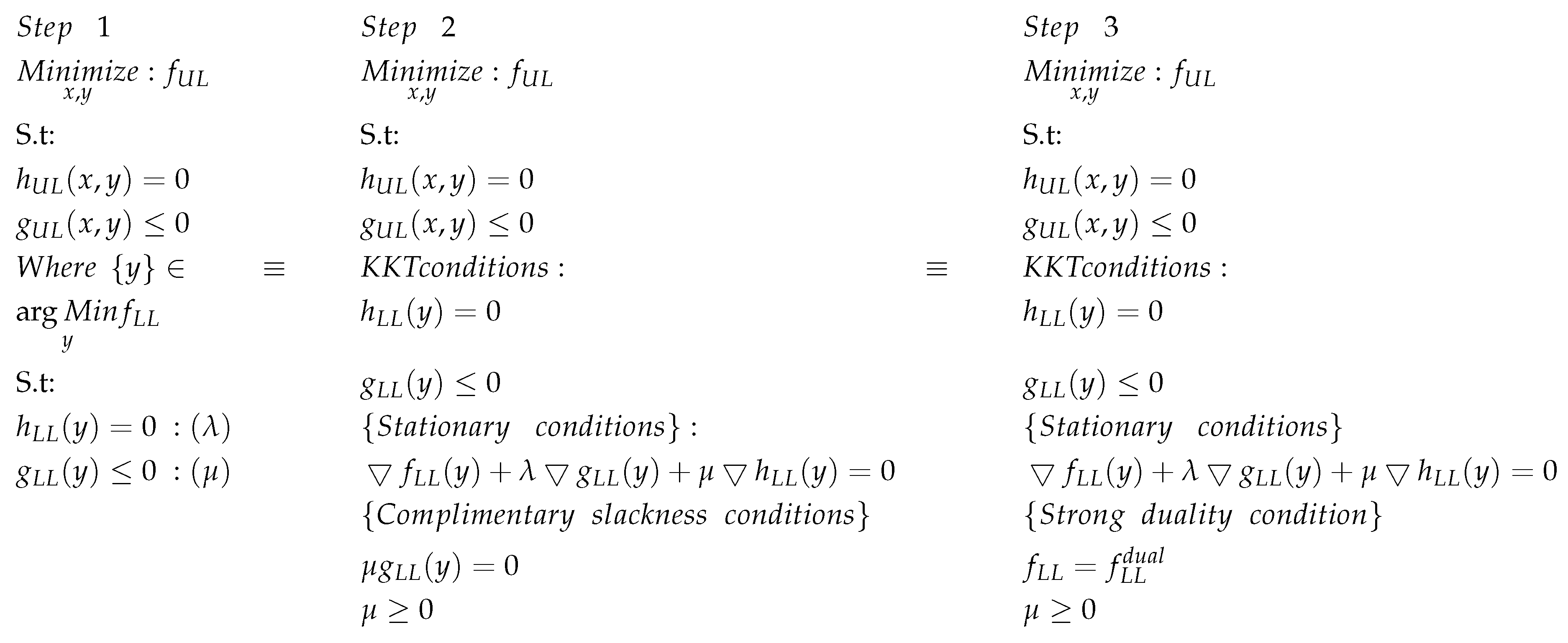
The proposed model is a bilevel mixed integer problem. Bilevel programming models are a powerful tool for problems with multiple-criteria decision-making models. Such models can be solved in various ways and one of the them is by reformulating the given bilevel model into a one-level model. The reformulation is illustrated in Figure 1. Step 1 shows the original bilevel formulation. The lower level is a linear problem and therefore could be equivalently represented by the Karush-Kuhn-Taker (KKT) optimality conditions. KKT optimality conditions consist of primal feasibility equations, stationary conditions and complementary slackness conditions. This reformulation will not affect the optimality since the KKT conditions are both necessary and sufficient [34]. The result of replacing the lower level problem by its KKT conditions is shown Step 2. However, the optimization problem in Step 2 is non-linear and therefore the complementary slackness conditions are replaced by the strong duality condition which implies that $f_{UL}^{☆}=f_{UL}^{☆dual}$. The final reformulated problem is shown in Step 3.

The reformulation steps described above were applied on the independent investment planing problem (30)–(35). The model was transformed from a bilevel mixed integer non-linear model into an equivalent one-level mixed integer non-linear problem. Stationary conditions and complementary slackness conditions for lower level problem (34) are derived in the Appendix of this paper. Two set of non-linearities were identified. The following sections explain how these non-linearities can be reformulated.

2.3. Strong Duality Condition

One set of non-linearities appears in the strong duality conditions of the reformulated one-level problem and are reformulated using the big-M approach.

$$\begin{array}{c}\sum _{s,p}[\sum _d(D_d^{max}(\uparrow {\overline{\omega }}_{d,p,s}+\downarrow {\overline{\omega }}_{d,p,s})+\sum _n{I}_{n,d}{D}_{d,p}{\lambda }_{n,p,s})+\sum _{w}w{p}_{p,s}{G}_w{\overline{\nu }}_{w,p,s}+\sum _j(G_j^{max}{\overline{\nu }}_{j,p,s}+\hfill \\ R{U}_j^{max}{\overline{\kappa }}_{j,p,s}+R{D}_j^{max}{\underline{\kappa }}_{j,p,s}-\sum _j{G}_j^{min}{\underline{\nu }}_{j,p,s})+\sum _h(G_h^{max}{\overline{\nu }}_{h,p,s}+R{U}_h^{max}{\overline{\kappa }}_{h,p,s}+R{D}_h^{max}{\underline{\kappa }}_{h,p,s}-G_h^{min}{\underline{\nu }}_{h,p,s}+\hfill \\ V_h^{max}{\overline{\sigma }}_{h,p,s}-V_h^{min}{\underline{\sigma }}_{h,p,s}+U_h^{max}{\overline{\vartheta }}_{h,p,s}+S_h^{max}{\overline{\theta }}_{h,p,s}+f{l}_{h,k,l}{\lambda }_{h,p,s}^{res})+\sum _n\Theta ({\overline{\rho }}_{n,p,s}+{\underline{\rho }}_{n,p,s})+\hfill \\ \sum _{n,m}{T}_{n,m}^{max}({\underline{\mu }}_{n,m,p,s}+{\overline{\mu }}_{n,m,p,s})+\underset{L1}{\underbrace{{\displaystyle \sum _e}{G}_e^{max}\underset{{\widehat{\xi }}_{e,p,s}^{ch}}{\underbrace{{\overline{\xi }}_{e,p,s}^{ch}{y}_{e,t}}}}}+\underset{L2}{\underbrace{{\displaystyle \sum _e}{G}_e^{max}\underset{{\widehat{\xi }}_{e,p,s}^{dch}}{\underbrace{{\overline{\xi }}_{e,p,s}^{dch}{y}_{e,t}}}}}+\underset{L3}{\underbrace{{\displaystyle \sum _e}{SOC}_e^{max}.\underset{{\widehat{\gamma }}_{e,p,s}^u}{\underbrace{{\overline{\gamma }}_{e,p,s}{y}_{e,t}}}}}-\hfill \\ \underset{L4}{\underbrace{{\displaystyle \sum _e}{SOC}_e^{min}.\underset{{\widehat{\gamma }}_{e,p,s}^l}{\underbrace{{\underline{\gamma }}_{e,p,s}{y}_{e,t}}}}}]-\sum _{t}R{G}^{min}\sum _{d,k,l}{D}_{d,p}{\beta }_t=-\sum _t(\psi \sum _s{\pi }_s(\sum _{k,l}{A}_{p,s}-\sum _k{B}_{k,t,s})\hfill \\ +\sum _w{C}_{w,t}(G_{w,t}^{max}-G_{w,t-1}^{max}))\hfill \\ +\sum _w{C}_{w,t}(G_{w,t}^{max}-G_{w,t-1}^{max}))\hfill \end{array}$$

(36)

The non-linear terms L1, L2, L3 and L4 can be reformulated by introducing new variables ${\widehat{\xi }}_{e,p,s}^{ch}$, ${\widehat{\xi }}_{e,p,s}^{dch}$, ${\widehat{\gamma }}_{e,p,s}^u$, ${\widehat{\gamma }}_{e,p,s}^l$ and using big-M reformulation technique. Stationary conditions and complementary slackness conditions for lower level problem (34) used in the linearizion process are derived as in Equations (A1)–(A16) and (A17)–(A49) respectively in the Appendix of this paper.

$$\begin{array}{c}{\widehat{\xi }}_{e,p,s}^{ch}-{\overline{\xi }}_{e,p,s}^{ch}\le M(1-y_{e,t})\forall e,p,s\hfill \\ {\widehat{\xi }}_{e,p,s}^{ch}\le M{y}_{e,t}\forall e,p,s\hfill \\ {\widehat{\xi }}_{e,p,s}^{ch}\ge 0\forall e,p,s\hfill \end{array}\}L1$$

(37)

$$\begin{array}{c}{\widehat{\xi }}_{e,p,s}^{dch}-{\overline{\xi }}_{e,p,s}^{dch}\le M(1-y_{e,t})\forall e,p,s\hfill \\ {\widehat{\xi }}_{e,p,s}^{dch}\le M{y}_{e,t}\forall e,p,s\hfill \\ {\widehat{\xi }}_{e,p,s}^{dch}\ge 0\forall e,p,s\hfill \end{array}\}L2$$

(38)

$$\begin{array}{c}{\widehat{\gamma }}_{e,p,s}^u-{\overline{\gamma }}_{e,p,s}\le M(1-y_{e,t})\forall e,p,s\hfill \\ {\widehat{\gamma }}_{e,p,s}^u\le M{y}_{e,t}\forall e,p,s\hfill \\ {\widehat{\gamma }}_{e,p,s}^u\ge 0\forall e,p,s\hfill \end{array}\}L3$$

(39)

$$\begin{array}{c}{\widehat{\gamma }}_{e,p,s}^l-{\underline{\gamma }}_{e,p,s}\le M(1-y_{e,t})\forall e,p,s\hfill \\ {\widehat{\gamma }}_{e,p,s}^l\le M{y}_{e,t}\forall e,p,s\hfill \\ {\widehat{\gamma }}_{e,p,s}^l\ge 0\forall e,p,s\hfill \end{array}\}L4$$

(40)

Big-M reformulation technique is used to convert a logical constraint into a set of linear constraints corresponding to the same feasible set. If the disjunctive parameter is chosen carefully then the reformulated problem will be equivalent to the original one. The big-M reformulation does not affect the size of the problem. However, the disjunctive parameters involved in the reformulation create computational issues for the solver. A disjunctive parameter that is not tuned affects the convergence of the problem [35]. The literature provides several methods to tune the big-M parameter. The methodologies for tuning big-M can be found in [35,36]. The methods are proved to provide good approximations of the big-M parameters under certain conditions but additional large scale optimization problems should be solved for each case and the optimality still cannot be guaranteed. The problem of the disjunctive parameter tuning becomes especially hard when the reformulation involves variables without physical upper or lower limits which is the case in our proposed model. In this paper we use a simple iterative method to tune big-M parameters. We iteratively solve the proposed model while increasing the big-M parameter till it does not affect the solution of the problem.

2.4. Reformulation of the Objective Function

Another set of non-linearities ${\lambda }_{n,p,s}{I}_{n,e}(g_{e,p,s}^{dch}-g_{e,p,s}^{ch})$ is found in objective function (30) and can be linearized following algebraic manipulation steps as shown below.

First step is to express ${\lambda }_{n,p,s}$ as a linear combination of other decision variables using stationary conditions of the lower level problem (A13) and (A14)

$$\begin{array}{c}\sum _{p,e}{\lambda }_{n,p,s}{I}_{n,e}(g_{e,p,s}^{dch}-g_{e,p,s}^{ch})\stackrel{\left(A13\right),\left(A14\right)}{=}\sum _{p,e}\left(\right(-\psi {\pi }_{s}m{c}_e+1/{ϵ}_e{\lambda }_{e,p,s}^{SOC}-{\underline{\xi }}_{e,p,s}^{dch}\hfill \\ +{\overline{\xi }}_{e,p,s}^{dch})g_{e,p,s}^{dch}+(-\psi {\pi }_{s}m{c}_e-{ϵ}_e{\lambda }_{e,p,s}^{SOC}-{\underline{\xi }}_{e,p,s}^{ch}+{\overline{\xi }}_{e,p,s}^{ch})g_{e,p,s}^{ch})\forall s\hfill \end{array}$$

(41)

Using complementary slackness conditions (A32)–(A35) for Equations (28) and (29) respectively we can further simplify the previous algebraic expression (41) as in (42):

$$\begin{array}{c}\sum _{p,e}((-\psi {\pi }_{s}m{c}_e+1/{ϵ}_e{\lambda }_{e,p,s}^{SOC})g_{e,p,s}^{dch}+G_e^{max}{\overline{\xi }}_{e,p,s}^{dch}+(-\psi {\pi }_{s}m{c}_e-{ϵ}_e{\lambda }_{e,p,s}^{SOC})g_{e,p,s}^{ch}+G_e^{max}{\overline{\xi }}_{e,p,s}^{ch})=\hfill \\ \sum _{p,e}(G_e^{max}({\overline{\xi }}_{e,p,s}^{dch}+{\overline{\xi }}_{e,p,s}^{ch})-\psi {\pi }_{s}m{c}_e(g_{e,p,s}^{dch}+g_{e,p,s}^{ch})-{\lambda }_{e,p,s}^{SOC}({ϵ}_e{g}_{e,p,s}^{ch}-1/{ϵ}_e{g}_{e,p,s}^{dch}))\hfill \end{array}$$

(42)

Equation (42) still contains non-linear term ${\lambda }_{e,p,s}^{SOC}({ϵ}_e{g}_{e,p,s}^{ch}-1/{ϵ}_e{g}_{e,p,s}^{dch})$. Thus, we apply additional algebraic manipulations. We first use energy balance constraint of energy storage (7) and express the charge and discharge variables $g_{e,p,s}^{ch}$ and $g_{e,p,s}^{dch}$ through state of charge variables $SO{C}_{e,t,k,l,s}$ and then we use stationary condition (A15) to represent the primary state of charge variables $SO{C}_{e,t,k,l,s}$ through linear combination of Lagrange multipliers.

$$\begin{array}{c}\sum _{p,e}{\lambda }_{e,p,s}^{SOC}({ϵ}_e{g}_{e,p,s}^{ch}-1/{ϵ}_e{g}_{e,p,s}^{dch})\stackrel{\left(7\right)}{=}\sum _{p,e}\left({\lambda }_{e,p,s}^{SOC}(SO{C}_{e,p,s}-{\varphi }_{e}SO{C}_{e,t,k,l-1,s})\right)=\hfill \\ \sum _{p,e}\left(SO{C}_{e,p,s}({\lambda }_p^{SOC}-{\varphi }_e{\lambda }_{e,t,k,l+1,s}^{SOC})\right)\stackrel{\left(A15\right)}{=}\sum _{p,e}\left(SO{C}_{e,p,s}(-{\overline{\gamma }}_{e,p,s}+{\underline{\gamma }}_{e,p,s}-\psi {\pi }_{s}F{C}_{k,t}{\rm Y}(l=L))\right)\forall s\hfill \end{array}$$

(43)

Using complementary slackness conditions (A36) and (A37) for Equation (18) we can simplify Equation (43) and replace the rest of the non-linear terms through linear combination of linear terms as in (44).

$$\sum _{p,e}(-SO{C}_e^{max}{\widehat{\gamma }}_{e,p,s}^u+SO{C}_e^{min}{\widehat{\gamma }}_{e,p,s}^l-\psi {\pi }_{s}F{C}_{k,t}SO{C}_{e,L,k,t,s}{\rm Y}(l=L))\forall s$$

(44)

By combining the algebraic expressions obtained in (42) and (44) we can now present the non-linear term ${\lambda }_{n,p,s}{I}_{n,e}(g_{e,p,s}^{dch}-g_{e,p,s}^{ch})$ through linear combination of linear terms as in (45)

$$\begin{array}{c}\sum _{p,e}\left({\lambda }_{n,p,s}{I}_{n,e}(g_{e,p,s}^{dch}-g_{e,p,s}^{ch})\right)\stackrel{\left(42\right),\left(44\right)}{=}\sum _{p,e}(G_e^{max}({\widehat{\xi }}_{e,p,s}^{dch}+{\widehat{\xi }}_{e,p,s}^{ch})-\psi {\pi }_{s}m{c}_e(g_{e,p,s}^{dch}+g_{e,p,s}^{ch})\hfill \\ +SO{C}_e^{max}{\widehat{\gamma }}_{e,p,s}^u-SO{C}_e^{min}{\widehat{\gamma }}_{e,p,s}^l+\psi {\pi }_{s}F{C}_{k,t}SO{C}_{e,l,k,t,s}{\rm Y}(l=L))\forall s\hfill \end{array}$$

(45)

2.5. One-Level Problem Formulation

The initial bilevel problem is now transformed into a one-level mixed integer linear problem, which is repeated here for the sake of clarity.

$$\begin{array}{c}\underset{{\Omega }_s\cup {\Omega }_p}{Maximize}:\hfill \\ f_{UL}=\sum _{e,t}P{w}_t(\psi \sum _{l,k,s}{\pi }_{s}W(p,e,s)-C_{e,t}(y_{e,t}-y_{e,t-1}))\hfill \end{array}$$

(46)

S.t:

$$\begin{array}{c}W(p,e,s)=G_e^{max}({\widehat{\xi }}_{e,p,s}^{dch}+{\widehat{\xi }}_{e,p,s}^{ch})-(\psi {\pi }_s+1)m{c}_e(g_{e,p,s}^{dch}+g_{e,p,s}^{ch})+SO{C}_e^{max}{\widehat{\gamma }}_{e,p,s}^u-SO{C}_e^{min}{\widehat{\gamma }}_{e,p,s}^l\hfill \\ +(\psi {\pi }_s+1)F{C}_{k,t}SO{C}_{e,L,k,t,s}\hfill \end{array}$$

(47)

$$y_{e,t}\ge y_{e,t-1}\forall e,t$$

(48)

$$\psi \sum _{t^{*}=t+1,k,l,e}^{t+PBP}{\pi }_{s}W(p,e,s)\ge \sum _e{C}_{e,t}(y_{e,t}-y_{e,t-1})\forall t$$

(49)

$$\psi \sum _{p,e,s}{\pi }_{s}W(p,e,s)\ge IR\sum _{t,e}{C}_{e,t}(y_{e,t}-y_{e,t-1})$$

(50)

$$\left(6\right)-\left(29\right)$$

(51)

{Stationary condition}

$$\left(A1\right)-\left(A16\right)$$

(52)

{Strong duality condition}

$$\begin{array}{c}\sum _{s,p}[\sum _d(D_d^{max}(\uparrow {\overline{\omega }}_{d,p,s}+\downarrow {\overline{\omega }}_{d,p,s})+\sum _n{I}_{n,d}{D}_{d,p}{\lambda }_{n,p,s})+\sum _{w}w{p}_{p,s}{G}_w{\overline{\nu }}_{w,p,s}+\sum _j(G_j^{max}{\overline{\nu }}_{j,p,s}+\hfill \\ R{U}_j^{max}{\overline{\kappa }}_{j,p,s}+R{D}_j^{max}{\underline{\kappa }}_{j,p,s}-\sum _j{G}_j^{min}{\underline{\nu }}_{j,p,s})+\sum _h(G_h^{max}{\overline{\nu }}_{h,p,s}+R{U}_h^{max}{\overline{\kappa }}_{h,p,s}+R{D}_h^{max}{\underline{\kappa }}_{h,p,s}-G_h^{min}{\underline{\nu }}_{h,p,s}+\hfill \\ V_h^{max}{\overline{\sigma }}_{h,p,s}-V_h^{min}{\underline{\sigma }}_{h,p,s}+U_h^{max}{\overline{\vartheta }}_{h,p,s}+S_h^{max}{\overline{\theta }}_{h,p,s}+f{l}_{h,k,l}{\lambda }_{h,p,s}^{res})+\sum _n\Theta ({\overline{\rho }}_{n,p,s}+{\underline{\rho }}_{n,p,s})+\hfill \\ \sum _{n,m}{T}_{n,m}^{max}({\underline{\mu }}_{n,m,p,s}+{\overline{\mu }}_{n,m,p,s})+\sum _e({SOC}_e^{max}{\widehat{\gamma }}_{e,p,s}^u-{SOC}_e^{min}{\widehat{\gamma }}_{e,p,s}^l+G_e^{max}({\widehat{\xi }}_{e,p,s}^{ch}+{\widehat{\xi }}_{e,p,s}^{dch}))]-\hfill \\ \sum _{t}R{G}^{min}\sum _{d,k,l}{D}_{d,p}{\beta }_t=-\sum _t(\psi \sum _s{\pi }_s(\sum _{k,l}{A}_{p,s}-\sum _k{B}_{k,t,s})+\sum _w{C}_{w,t}(G_{w,t}^{max}-G_{w,t-1}^{max}))\hfill \end{array}$$

(53)

{Big-M reformulation constraints}

$$\left(37\right)-\left(40\right)$$

(54)

where:

$$\begin{array}{c}{\Omega }_p=\{{\lambda }_n,{\lambda }_e^{SOC},{\lambda }_h^{res},\tau 0_w,{\tau }_w,{\varphi }_w,{\underline{\xi }}_e^{ch},{\overline{\xi }}_e^{ch},{\underline{\xi }}_e^{dch},{\overline{\xi }}_e^{dch},{\underline{\mu }}_{n,m},{\overline{\mu }}_{n,m},{\overline{\sigma }}_h,{\underline{\sigma }}_h,{\underline{\nu }}_j,{\overline{\nu }}_j,{\underline{\kappa }}_h,{\overline{\kappa }}_h,{\underline{\kappa }}_j,{\overline{\kappa }}_j,\hfill \\ {\underline{\nu }}_w,{\overline{\nu }}_w,{\underline{\omega }}_d,{\overline{\omega }}_d,{\underline{\gamma }}_e,{\overline{\gamma }}_e,{\underline{\vartheta }}_h,{\overline{\vartheta }}_h,{\underline{\theta }}_h,{\overline{\theta }}_h,{\widehat{\gamma }}_e,{\widehat{\xi }}_e^{ch},{\widehat{\xi }}_e^{dch}\}\hfill \end{array}$$

3. Case Study

The case study tries to answer the following questions. First, how will the presence of energy storage investment option affect system operation cost, electricity prices and wind-based generation expansion? Second, how will the planning approach (centralized and decentralized) affect the investment decisions on energy storage and will the results be different for systems with congested transmission capacity? Third, can energy storage benefit from congestion in the system under decentralized planning? Therefore the following simulation steps were performed. First, the centralized planning model without energy storage investment possibility was simulated, Case 1. Second, energy storage investment option was added and centralized and decentralized planning were simulated under different flexibility set-ups, Case 2 and Case 3 respectively. Third, the second step was repeated for the systems with and without transmission congestion. In addition, a case study without renewable generation expansion was performed, Case 4. In this case study we fix renewable generation capacity in the level to satisfy renewable penetration target and simulate energy storage investment planning under both centralized and decentralized planning models.

The models from section II have been tested on the IEEE 30-node test system. The generation mix has been varied to obtain different flexibility levels of the system and compare optimal energy storage investments. In the first and second set-ups, which is referred to as the thermal system (T) and thermal system with demand response (T+D), the generation consists of thermal units and wind power in set-up T and thermal units, wind power and flexible demand in system T-D. In the third and fourth set-ups, which is referred to as the hydro-thermal (H-T) system and hydro-thermal system with flexible demand (H-T+D), some of the thermal units of T and T+D system respectively are replaced by hydro units. The total installed capacity of generation units remains the same; however, the total expected ramping capability of the system is changed based on the thermal unit characteristics. The generation mix and total expected ramping capability can be found in

Table 1. Test system input data.

	Thermal		Hydro-Thermal
	Capacity	Node	Capacity	Node
Thermal, (MW)	600	1, 2, 22, 27, 23, 13	300	1, 2, 23
Hydro, (MW)	-	-	300	22, 27
Wind, (MW)	100	5, 6	100	5, 6
Max. demand, (MW)	600	-	600	-
Flexible demand	10%	-	10%	-
Transmission limits, (MW)	100	-	100	-
Congested transmission limits, (MW)	70	-	70	-
Ramping capability, (MW)	300	-	420	-
Renewable generation target	20%	-	20%	-

.

The total expected ramping capability ($R\_Total$) of the system is measured in MW per minute and calculated as an expected maximum reserves which could be provided by each plant, energy storage and flexible demand. A formula is provided to calculate total expected ramping capability of the system:

$$\begin{array}{c}R\_Total=\sum _s{\pi }_s\frac{1}{T*l}\left(\sum _p\right(\sum _{j}min\{R{U}_j^{max},G_j^{max}-g_{j,p,s}\}+\sum _{h}min\{R{U}_h^{max},G_h^{max}-g_{h,p,s}\}\hfill \\ +\sum _e(SO{C}_{e,p,s}-SO{C}_e^{min})+\sum _d(D_d^{max}-\downarrow \Delta d_{d,p,s})\left)\right)\hfill \end{array}$$

(55)

The total expected ramping capability is used to compare the flexibility levels of different case study set-ups. It is calculated based on hourly available energy capacity of the thermal and hydro generation considering ramping limits and available energy which can be obtained through energy storage and demand response. Energy storage and demand response are considered to have very fast ramping capability and therefore no ramping limits are imposed on these sources of flexibility. However, it should be noted that this approach will not capture the full dynamics of energy limited resources such as hydro power, flexible demand and energy storage, but can be used to approximate the flexibility of the system. A more exact measurement of flexibility of the system is outside of the scope of this paper. The measurement is calculated based on the up-ramping capability of the system and a similar index can be calculated based on the down-ramping capability of the system. However, in this system, the down-ramping capability is always larger than the up-ramping capability (especially if consider possibility to curtail wind power) and is therefore not analyzed any further. The transmission capacity connecting wind-based generation with load were reduced in order to create congestion in the system and analyze the impact of additional flexibility and behaviour of both planning strategies. In addition, the systems with initially congested transmission capacity were compared to the cases where transmission capacity was increased and congestion was eliminated.

3.1. System Description

The IEEE 30-node test system was chosen to test and analyze presented investment models. The initial input data is presented in Table 1. The installed capacity is chosen to be almost the same as the peak demand in order to force additional investments into renewable generation. Practically, this situation reflects the decision to close large power plants in the system such as nuclear or coal and replace the required generation by investments into a wind-based generation and an additional flexibility source such as energy storage unit. In addition, the investments in renewable generation is ensured through lower limit constraint on expected generation from renewable generation.

A moment matching technique is used to generate the wind power generation scenarios [37]. The technique provides various advantages. The main one is that the technique allows to use a relatively few numbers of distinct scenarios and therefore reduces the computational difficulty for solving the stochastic program. The investment decisions in energy storage are made considering two different energy storage technologies available: compressed air energy storage (CAES) and batteries. Both of these technologies could be used for bulk energy storage, mature and commercially available. Each technology represented through a set of energy storage units of fixed energy capacity and power capability which could be invested in. The technical characteristics of each unit of each technology as well as the energy capacity and the power capability are presented in

Table 3. Energy storage characteristics.

Technology	CAES	Battery
Energy storage capacity, $SO{C}_e^{max}$, (MWh)	100	15
Power limit, $G_e^{max}$, (MW)	20	6
Energy conversion efficiency, ($\epsilon$)	0.75	0.85
Self discharge of energy storage, ($\eta$)	0.78	0.99
Initial state of charge	50%	50%
Capital cost, Energy, ($/kWh)	5	400
Capital cost, Power, ($/kW)	700	400
Maximum number of units	5	10

.

Case studies presented in this paper consider different levels of capital costs of energy storage. Initially, capital costs were assumed to be high to represent current state of the energy storage market. We expect a cost reduction each year of up to 5 %, i.e., $C_{e,t}=0.95C_{e,t-1}$, to take into account predicted reduction of the capital costs in the future and development of new technologies. The initial capital costs for the first year were taken from [15] for energy storage and from [38] for wind power. The costs were updated using the present worth factor based on (56) and parameters presented in

Table 2. Investment cost assumptions.

Parameter	Value
Annual inflation rate, (inf)	2%
Discount rate, (dis)	10%

and in

Table 4. Investment parameters.

Parameter	Value
Planning period, (T)	10 years
Investments return parameter, ($IR$)	1.2
Payback period limit, ($PBP$)	5
Short term operation period, (l)	74 h
Renewable penetration target year, ($RTY$)	5th year

.

$$P{w}_t=\frac{{(1+inf)}^t}{{(1+dis)}^t}$$

(56)

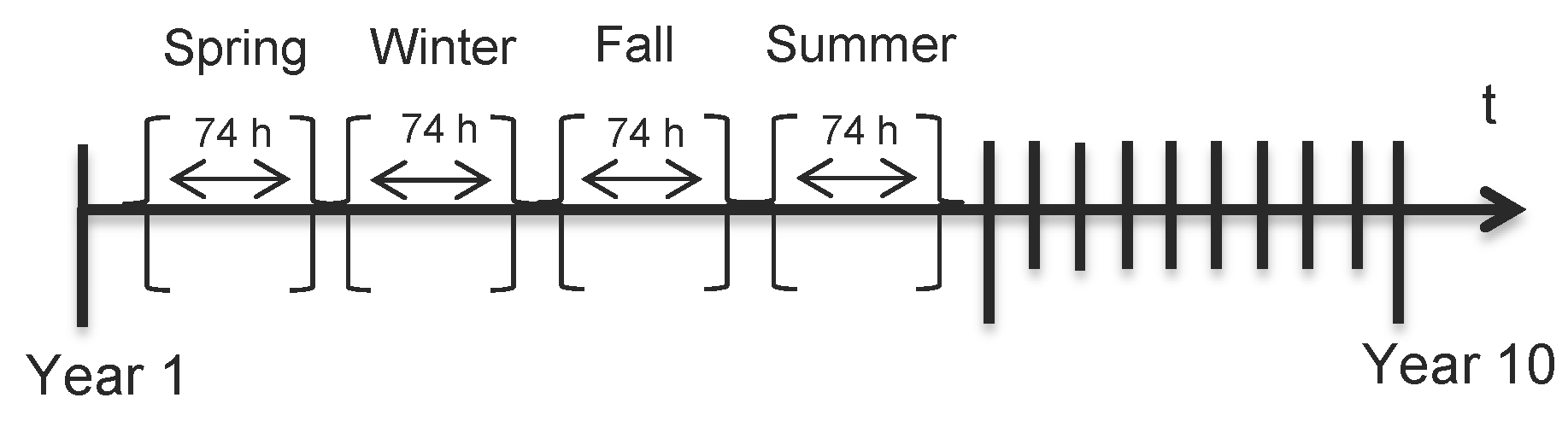
Thus, the investment decisions could be delayed for later periods when the conditions will be more financially favourable. Investment decision planning includes 10 consecutive periods which represent years. Each year consists of four consecutive operational periods which represent each season of that year. Figure 2 shows the time line for the operation planning and investments decisions.

For the hydro-thermal generation mixes the limits for hydro reservoirs at the end of the each operational period were set based on the outputs of the weekly schedule and are allowed to be deviated up to 10% of the scheduled amount for each operational period of each year. This was done to simulate long term hydro power scheduling and avoid overuse of hydropower.

3.2. Results and Discussions

Table 5. Case study results.

	Congested				Not Congested
	T	T+D	H-T	H-T+D	T	H-T
Case 1. Base case (no ES investments)
Available capacity, (MW)	600	600	600	600	600	600
Wind power investments, (MW)	288	274	273	271	281	271
Ramping capability, (MWh)	300	360	420	480	300	420
Number of congested lines	3	1	3	1	0	0
Curtailed wind, (%)	10	8	11	6	7	5
Std of price	14.2	13.1	5.2	5.7	13.3	4.5
Average price, ($)	52	45	32	32	45	34
Case 2. Centralized planning
Wind power investments, (MW)	241	235	232	238	248	236
Energy storage investments, (MW)	115	45	45	45	100	30
Ramping capability, (MWh)	390	390	455	510	384	447
Std of price	4.3	3.9	3.4	3.1	4.3	3.1
Average price, ($)	40	40	30	30	40	30
Number of congested lines	1	0	1	0	0	0
Curtailed wind, (%)	≥1	≥1	≥1	≥1	≥1	≥1
Case 3. Decentralized planning
Wind power investments, (MW)	257	241	273	271	270	271
Energy storage investments, (MW)	90	45	0	0	45	0
Ramping capability, (MWh)	330	390	420	480	390	420
Std of price	6.2	5.4	5.2	5.7	5.2	4.5
Average price, ($)	44	40	35	35	40	34
Number of congested lines	2	1	2	1	0	0
Curtailed wind, (%)	6	6	9	6	7	4
Case 4. Decentralized planning with fixed wind investments
Energy storage investments, (MW)	90	45	45	45	100	30
Ramping capability, (MWh)	330	390	420	480	384	447
Std of price	6.9	6.1	5.8	5.9	4.3	3.1
Average price, ($)	46	41	38	37	40	30
Number of congested lines	3	1	3	1	0	0
Curtailed wind, (%)	6.5	6.8	9	6	≥1	≥1

and

Table 6. Energy storage investment results. Bat: Battery.

	Congested				Not Congested
	Centralized		Decentralized		Centralized		Decentralized
	CAES	Bat.	CAES	Bat.	CAES	Bat.	CAES	Bat
Thermal system
Time period, (t)	t1	t1	-	t5	t1	t1	-	t5
Node, (n)	3	25	-	4, 6, 8	4	25	-	4, 8, 25
Number of units	1	6	-	1	1	3	-
Hydro-Thermal system
Time period, (t)	-	t1	-	-	-	t1	-	-
Node, (n)	-	3, 25, 15	-	-	-	3, 25	-	-
Number of units	-	3	-	-	-	2	-	-

present the results for the case studies listed above. Table 5 presents the summarized investment results and the influence of these investments on operation cost, renewable generation spillage and presence of congestion in the system. Table 6 presents more detailed data on energy storage investment, such as the time period when the investment was made, which technology was chosen and the node it was placed in.

First of all, the results show that energy storage could be a financially beneficial investment both, under centralized and decentralized planning. However, in hydro-thermal systems energy storage investments are not profitable for independent investors. No investments were made under decentralized planning in hydro-thermal systems while under centralized planning 45 MW of energy storage were installed which is 8% of the total installed generation capacity of the system. Considerable investments were made under decentralized planning in thermal only systems. 90 MW of energy storage consisting of batteries were installed compared to 115 MW of storage capacity consisting of CAES and a batteries under centralized planning. While decentralised planning ensures that the owner of energy storage system earns sufficient benefits in a fixed payback period time, the investments made are still beneficial for the whole system by reducing electricity prices and relieving transmission congestion. However, the benefits are much lower than under centralized planning and mainly due to lower investments in energy storage and as a consequence in renewable generation expansion. For example in the thermal only system the investments made under decentralized planning resulted in 12% price reduction compared to 20% price reduction under centralized planning while the standard deviation of the price was reduced from 12.6 to 6.2 in decentralized planning and till 4.3 under centralized planning. Curtailed wind remained relatively high (5%) under decentralized planning while centralized planning allowed to almost completely eliminate wind curtailment. Moreover energy storage investments reduced substantially installed capacity of the wind power generation which was required by renewable generation target set by the system. In centralized planning 115 MW of energy storage investment in thermal system helped to reduce required installed capacity of wind generation from 288 MW to 241 MW.

Another interesting observation was that in the system with congested transmission capacity, an independent profit maximizing energy storage owner will choose the placement of large energy storage units in such a way to keep the congestion in the system. On the other hand, under centralized planning more investments will be made just to relieve the congestion and reduce the renewable generation spillage and total operation cost. The difference is noticeable when comparing the system with three congested lines to the system without congestion. The average price and variability of the price is reduced under both centralized and decentralized planning with all generation mix set-ups while energy storage investments are also lower than in the case studies with congested lines with the same generation mix set-ups. For example the results in Table 6 show that similar quantities of energy storage were deployed under decentralized planning for congested and not congested systems but the nodes of placement were different. In the congested system under decentralized planning energy storage was placed at nodes 4, 6 and 8. In addition, the average price difference between centralized and decentralized planning was 9 % while in the non-congested system the price difference was equal to zero and the energy storage units were placed at nodes 4, 8 and 25. In centralized planning energy storage investments contribute to substantial reduction of wind power spillage and wind power generation investments which were forced by renewable generation target. Moreover, average price and price variability also were significantly lowered by additional energy storage investments. Decentralized planning also resulted in energy storage investments however the overall benefits of the system from these investments was lower.

In addition decentralized planning of energy storage especially in already congested systems can have a negative impact on system operation and further congested power system. This could be the case when variable renewable generation is planned beforehand and the flexibility requirements are set afterword. Thus, the flexibility providers can benefit from strategic placement and internalize existing system congestion. However, the results of the case studies show that independent energy storage investments will still contribute to congestion relief but in much lower volumes than in centralized planning. Congestion relief under decentralized planning is mainly due to the assumption that system operator follows energy storage investment decision and expands renewable generation according to the decision made on upper level. Thus, energy storage owner can not congest system further and considerably influence on locational marginal prices at the congested nodes. The case study Case 4 also proves this. The investments on energy storage when renewable generation capacity was fixed considerably increased price volatility and did not relieve congestion at all.

In addition, the investments in energy storage under independent investment planning were done predominately in batteries while in centralized planning the investments also include compressed air energy storage (CAES). Under centralized planning both congested and non-congested systems deployed one CAES unit while none of the case studies under decentralized planning invested in CAES. The large size of CAES and associated high total capital cost makes it harder for independent investors to get the payback of the investments in reasonable time. Thus, the payback limit constraints introduced in independent planning model restricts these investments.

Based on the case study results we can suggest that centralized ownership model provides more benefits to the power systems and ensures an effective short-term operation. However, current regulations existing in Europe prohibit the use of energy storage technologies for energy arbitrage if they are owned by the system operator. Thus, decentralized ownership model is the only valid option to provide energy arbitrage. The decentralized ownership of energy storage without proper regulation may potentially congest the system and result in inefficient development of power system and reduced deployments of renewable generation such as wind. Additional research on various regulations on energy storage investments should be performed in order to fully answer the question who should be responsible for energy storage investments.

4. Conclusions

This paper presents two mathematical models for centralized and decentralized investment planning of energy storage and wind power generation expansion. The decentralized investment planning is formulated as MPEC model, where a single energy storage investor is interacting with a centralized operator representing a perfect market environment. Both models are useful to investigate the interactions between variability of renewable generation and the flexibility provided by energy storage. The models include a wide range of generation mixes which allows to model different types of the system with different flexibility levels just by varying the input parameters.The proposed models allow to evaluate the differences between centralized and decentralized planning. Additional constraint on investments return and payback periods express the constraints of a profit maximizing company when it faces investment planning decisions. The models were applied on a case studies with various levels of flexibility and different levels of congestion in transmission capacity.

The following main conclusions were obtained from the case studies:

• First, energy storage can be beneficial to the whole system by reducing spillage of renewable generation and relieving congestion of transmission capacity under both centralized and decentralized planning approaches. However, there are still a big gap between centralized and decentralized planning approaches. More investments are made under centralized planning and the cost and the average price reduction under centralized planning is much higher.
• Second, if treated as a market asset (decentralized planning) energy storage can profit from strategically placing energy storage units and contribute on increase to transmission congestion of power system and additional wind spillage.
• Third, negative impact of strategic behavior of energy storage can be reduced if renewable generation decisions are taken simultaneously.
• Fourth, the case studies demonstrate that decentralized unregulated allocation planning for energy storage potentially may cause congestion in the system. Thus, additional studies on proper regulation for energy storage is necessary.

The gap between centralized and decentralized planning could be reduced if independent energy storage owner were able to have additional profits apart from energy arbitrage. An additional profit stream could increase the investments in energy storage under decentralized planning. This is the case especially in hydro-thermal system where investments in energy storage are generally less profitable under both centralized and decentralized investment planning. The revenue streams can include participation in balancing markets and provision of reserves. On the other hand increasing penetration of variable renewable generation will also increase the potential profitability and need in energy storage systems. Based on case study results energy storage considerably reduces wind spillage and therefore coordinated investment planning with renewable generation might increase investments in energy storage even under decentralized planning. Otherwise, in order to ensure sufficient flexibility in the system grid, the owner should be eligible and responsible for investments in energy storage. For example such a strategy was chosen in California and Oregon by passing energy storage mandates on energy storage installations.

Future research steps could be identified as the following.

• First, proposed decentralized model considers monopoly on energy storage investments and does not take into account additional competition from investments made on other flexibility sources such as hydro, flexible demand or flexible generators. Thus, an EPEC model could be developed to coordinate the investment and evaluate the dependency.
• Second, the models consider only one revenue stream which comes from providing energy arbitrage, however additional revenue streams such as provision of balancing services should be also considered to further evaluate the profitability of energy storage.
• Third, the initial formulation of the decentralized planning model is presented as a mixed integer non-linear bilevel model and later reformulated as a mixed integer linear one-level problem. The suggested technique for reformulation and linearization reduces the complexity of the model and makes it possible to find an optimal solution with reasonable computational time. However, the linearized model is still complex and a higher number of nodes and decision variables will increase the computational time. In order to apply the models to larger systems, it could be beneficial to investigate decomposition techniques (ex. Benders decomposition).
• Fourth, the choice of the number of days and operational hours also affects the computational time and the energy storage evaluation require rather large operational period to observe the charge and discharge cycles. Thus, the selection of the critical operational periods for energy storage evaluation is also a subject for future research.

References

- REN21. Renewables 2016 Global Status Report; REN21 Secretariat: Paris, France, 2016. [Google Scholar]
- Holttinen, H.; Milligan, M.; Ela, E.; Menemenlis, N.; Dobschinski, J.; Rawn, B.; Bessa, R.; Flynn, D.; Gomez-Lazaro, E.; Detlefsen, N. Methodologies to Determine Operating Reserves Due to Increased Wind Power. IEEE Trans. Sustain. Energy 2012, 3, 713–723. [Google Scholar] [CrossRef]
- Hirth, L.; Ueckerdt, F.; Edenhofer, O. Integration costs revisited—An economic framework for wind and solar variability. Renew. Energy 2015, 74, 925–939. [Google Scholar] [CrossRef]
- Department of Energy. Global Energy Storage Database. Available online: https://www.energystorageexchange.org/ (accessed on 15 January 2018).
- International Energy Agency. Technology Roadmap—Solar Photovoltaic Energy; International Energy Agency: Paris, France, 2014. [Google Scholar]
- Eyer, J.; Corey, G. Energy Storage for the Electricity Grid: Benefits and Market Potential Assessment Guide; Sandia National Laboratories: Albuquerque, NM, USA, 2010. [Google Scholar]
- Akhil, A.A.; Huff, G.; Currier, A.B.; Kaun, B.C.; Rastler, D.M.; Chen, S.B.; Cotter, A.L.; Bradshaw, D.T.; Gauntlett, W.D. DOE/EPRI 2013 Electricity Storage Handbook in Collaboration with NRECA; Sandia National Laboratories: Albuquerque, NM, USA, 2013. [Google Scholar]
- Das, T.; Krishnan, V.; McCalley, J.D. Assessing the benefits and economics of bulk energy storage technologies in the power grid. Appl. Energy 2015, 139, 104–118. [Google Scholar] [CrossRef]
- Heydarian-Forushani, E.; Golshan, M.; Siano, P. Evaluating the benefits of coordinated emerging flexible resources in electricity markets. Appl. Energy 2017, 199, 142–154. [Google Scholar] [CrossRef]
- Qin, M.; Chan, K.W.; Chung, C.Y.; Luo, X.; Wu, T. Optimal planning and operation of energy storage systems in radial networks for wind power integration with reserve support. IET Gener. Transm. Distrib. 2016, 10, 2019–2025. [Google Scholar] [CrossRef]
- Liu, J.; Wen, J.; Yao, W.; Long, Y. Solution to short-term frequency response of wind farms by using energy storage systems. IET Renew.e Power Gener. 2016, 10, 669–678. [Google Scholar] [CrossRef]
- Edmunds, R.; Cockerill, T.; Foxon, T.; Ingham, D.; Pourkashanian, M. Technical benefits of energy storage and electricity interconnections in future British power systems. Energy 2014, 70, 577–587. [Google Scholar] [CrossRef]
- Zucker, A.; Hinchliffe, T.; Spisto, A. Assessing Storage Value in Electricity Markets; JRC Scientific and Policy Report; Joint Research Centre: Brussels, Belgium, 2013. [Google Scholar]
- Schoenung, S. Energy Storage Systems Cost Update; Sandia National Laboratories: Albuquerque, NM, USA, 2011. [Google Scholar]
- Zakeri, B.; Syri, S. Electrical energy storage systems: A comparative life cycle cost analysis. Renew. Sustain. Energy Rev. 2015, 42, 569–596. [Google Scholar] [CrossRef]
- Chen, H.; Zhang, R.; Li, G.; Bai, L.; Li, F. Economic dispatch of wind integrated power systems with energy storage considering composite operating costs. IET Gener. Transm. Distrib. 2016, 10, 1294–1303. [Google Scholar] [CrossRef]
- Hu, Z.; Jewell, W.T. Optimal generation expansion planning with integration of variable renewables and bulk energy storage systems. In Proceedings of the 2013 1st IEEE Conference on Technologies for Sustainability (SusTech), Portland, OR, USA, 1–2 August 2013; pp. 1–8. [Google Scholar]
- Qiu, T.; Xu, B.; Wang, Y.; Dvorkin, Y.; Kirschen, D. Stochastic Multi-Stage Co-Planning of Transmission Expansion and Energy Storage. IEEE Trans. Power Syst. 2016, 32, 643–651. [Google Scholar] [CrossRef]
- Dehghan, S.; Amjady, N. Robust Transmission and Energy Storage Expansion Planning in Wind Farm- Integrated Power Systems Considering Transmission Switching. IEEE Trans. Sustain. Energy 2016, 7, 765–774. [Google Scholar] [CrossRef]
- Solomon, A.; Kammen, D.M.; Callaway, D. The role of large-scale energy storage design and dispatch in the power grid: A study of very high grid penetration of variable renewable resources. Appl. Energy 2014, 134, 75–89. [Google Scholar] [CrossRef]
- Makarov, Y.V.; Du, P.; Kintner-Meyer, M.C.; Jin, C.; Illian, H.F. Sizing energy storage to accommodate high penetration of variable energy resources. IEEE Trans. Sustain. Energy 2012, 3, 34–40. [Google Scholar] [CrossRef]
- Alnaser, S.W.; Ochoa, L.F. Optimal Sizing and Control of Energy Storage in Wind Power-Rich Distribution Networks. IEEE Trans. Power Syst. 2016, 31, 2004–2013. [Google Scholar] [CrossRef]
- Dvorkin, Y.; Fernandez-Blanco, R.; Kirschen, D.S.; Pandzic, H.; Watson, J.P.; Silva-Monroy, C.A. Ensuring Profitability of Energy Storage. IEEE Trans. Power Syst. 2016, 31, 611–623. [Google Scholar] [CrossRef]
- Fern, R.; Dvorkin, Y.; Xu, B.; Wang, Y.; Kirschen, D.S. Energy Storage Siting and Sizing in the WECC Area and the CAISO System; University of Washington: Seattle, DC, USA, 2016; pp. 1–31. [Google Scholar]
- Dvijotham, K.; Chertkov, M.; Backhaus, S. Storage sizing and placement through operational and uncertainty-aware simulations. In Proceedings of the Annual Hawaii International Conference on System Sciences, Waikoloa, HI, USA, 6–9 January 2014; pp. 2408–2416. [Google Scholar]
- Zhang, F.; Hu, Z.; Song, Y. Mixed-integer linear model for transmission expansion planning with line losses and energy storage systems. IET Gener. Transm. Distrib. 2013, 7, 919–928. [Google Scholar] [CrossRef]
- Wogrin, S.; Gayme, D.F. Optimizing Storage Siting, Sizing, and Technology Portfolios in Transmission- Constrained Networks. IEEE Trans. Power Syst. 2015, 30, 3304–3313. [Google Scholar] [CrossRef]
- Go, R.S.; Munoz, F.D.; Watson, J.P. Assessing the economic value of co-optimized grid-scale energy storage investments in supporting high renewable portfolio standards. Appl. Energy 2016, 183, 902–913. [Google Scholar] [CrossRef]
- Nasrolahpour, E.; Kazempour, S.J.; Zareipour, H.; Rosehart, W.D. Strategic Sizing of Energy Storage Facilities in Electricity Markets. IEEE Trans. Sustain. Energy 2016, 7, 1462–1472. [Google Scholar] [CrossRef]
- Cui, H.; Li, F.; Fang, X.; Chen, H.; Wang, H. Bi-Level Arbitrage Potential Evaluation for Grid-Scale Energy Storage Considering Wind Power and LMP Smoothing Effect. IEEE Trans. Sustain. Energy 2017. [Google Scholar] [CrossRef]
- Kazempour, S.J.; Conejo, A.J.; Ruiz, C. Generation Investment Equilibria With Strategic Producers; Part I: Formulation. IEEE Trans. Power Syst. 2013, 28, 2613–2622. [Google Scholar] [CrossRef]
- Grbovic, P. Energy Storage Technologies and Devices. In Ultra-Capacitors in Power Conversion Systems: Analysis, Modeling and Design in Theory and Practice; Wiley-IEEE Press: Hoboken, NJ, USA, 2014; p. 336. [Google Scholar]
- Ramos, T.P.; Marcato, A.L.M.; da Silva Brandi, R.B.; Dias, B.H.; da Silva Junior, I.C. Comparison between piecewise linear and non-linear approximations applied to the disaggregation of hydraulic generation in long-term operation planning. Int. J. Electr. Power Energy Syst. 2015, 71, 364–372. [Google Scholar] [CrossRef]
- Bertsekas, D.P. Nonlinear Programming; Athena Scientific Belmont: Belmont, MA, USA, 1999. [Google Scholar]
- Hooker, J. Logic-Based Methods for Optimization: Combining Optimization and Constraint Satisfaction; John Wiley & Sons: Hoboken, NJ, USA, 2011; Volume 2. [Google Scholar]
- Trespalacios, F.; Grossmann, I.E. Improved Big-M reformulation for generalized disjunctive programs. Comput. Chem. Eng. 2015, 76, 98–103. [Google Scholar] [CrossRef]
- Rubasheuski, U.; Oppen, J.; Woodruff, D.L. Multi-stage scenario generation by the combined moment matching and scenario reduction method. Oper. Res. Lett. 2014, 42, 374–377. [Google Scholar] [CrossRef]
- Breeze, P. Wind Power. Power Gener. Technol. 2014, 1, 223–242. [Google Scholar]
Figure 1.
One-level equivalent reformulation steps.
Figure 2.
Investment planning time line.