Mapping Mangroves Extents on the Red Sea Coastline in Egypt using Polarimetric SAR and High Resolution Optical Remote Sensing Data


Abstract
:1. Introduction
2. Materials and Methods
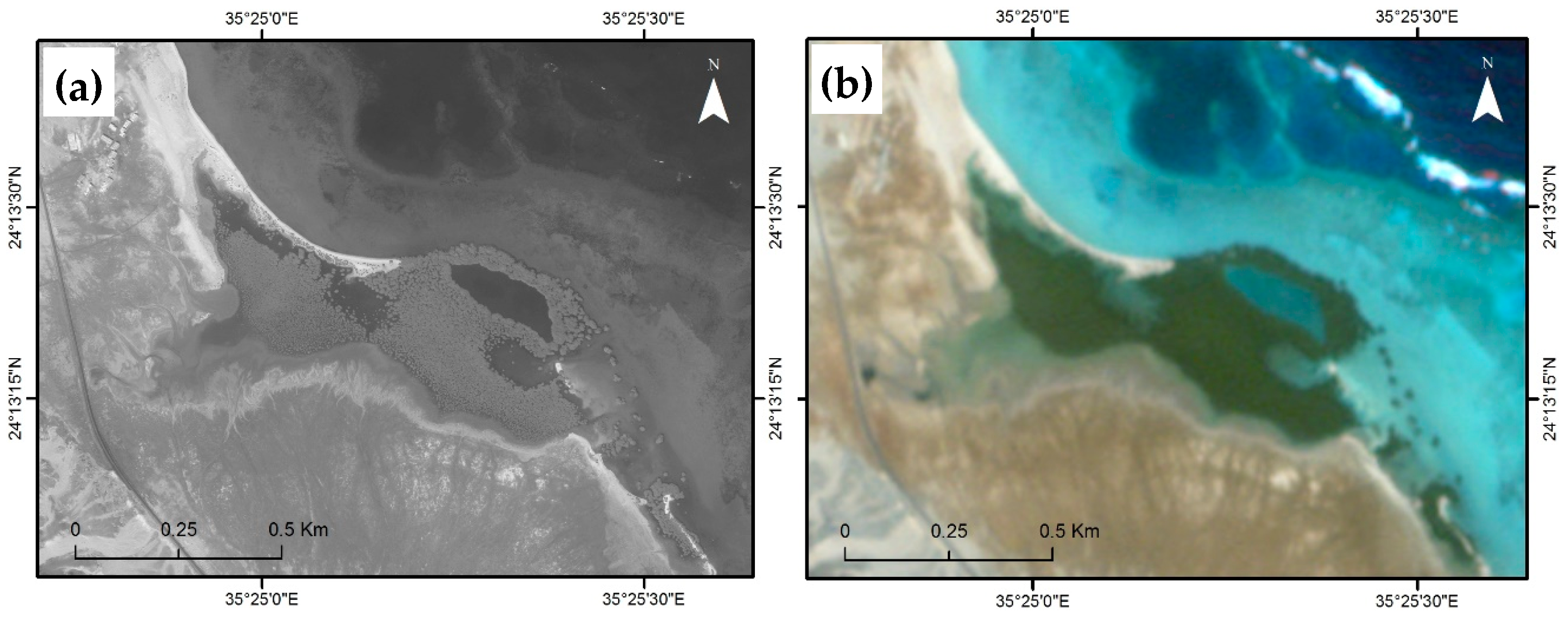
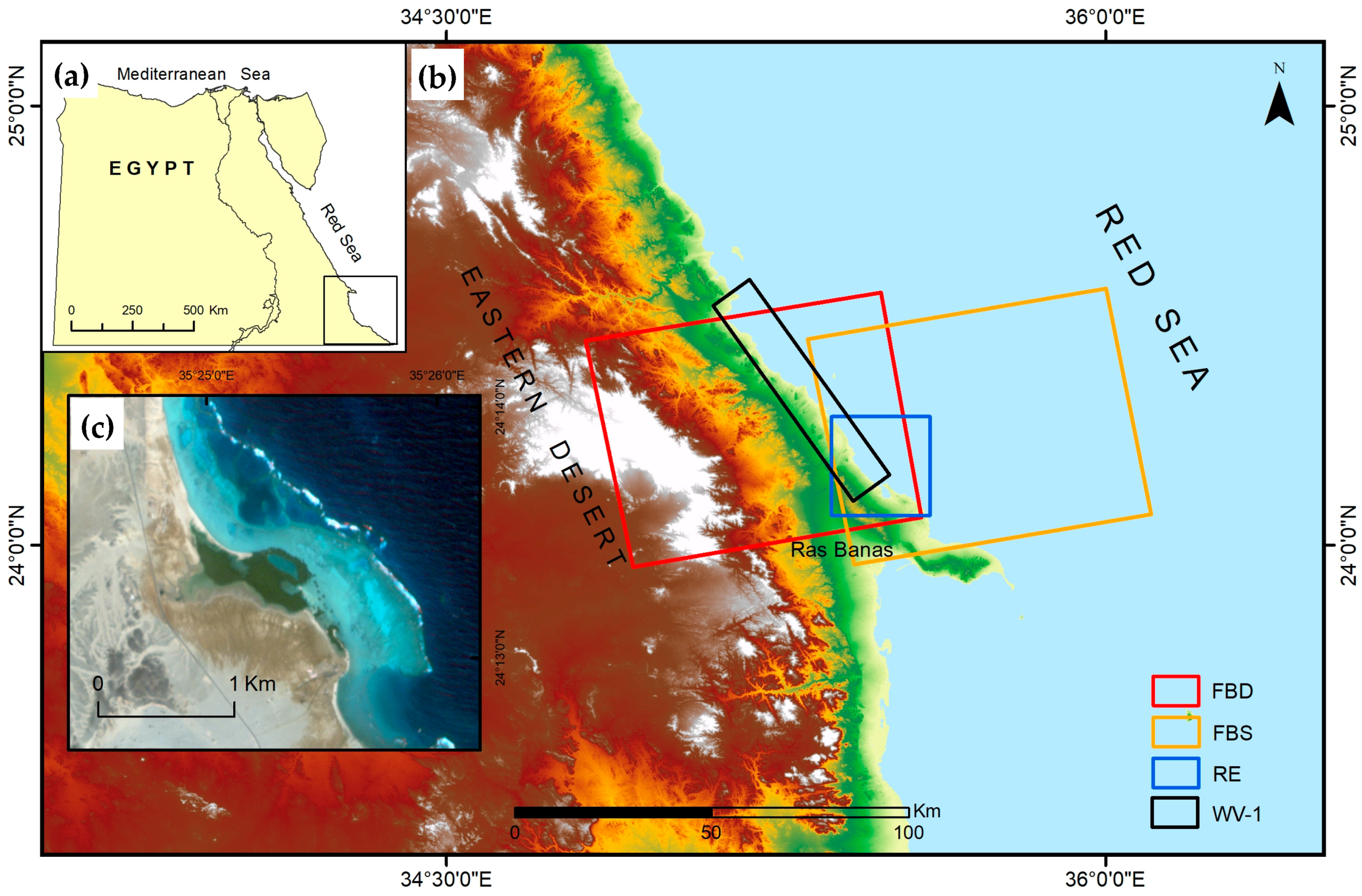
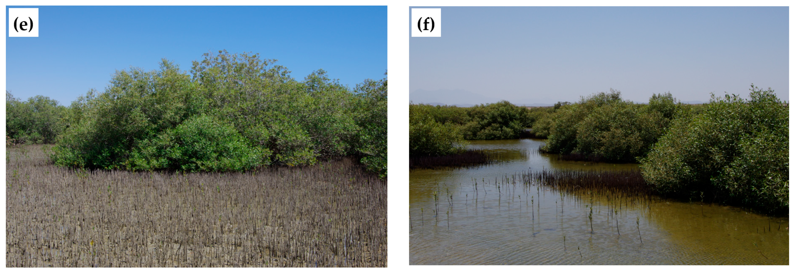
2.1. Study Area
2.2. Remote Sensing Data
Data Analysis
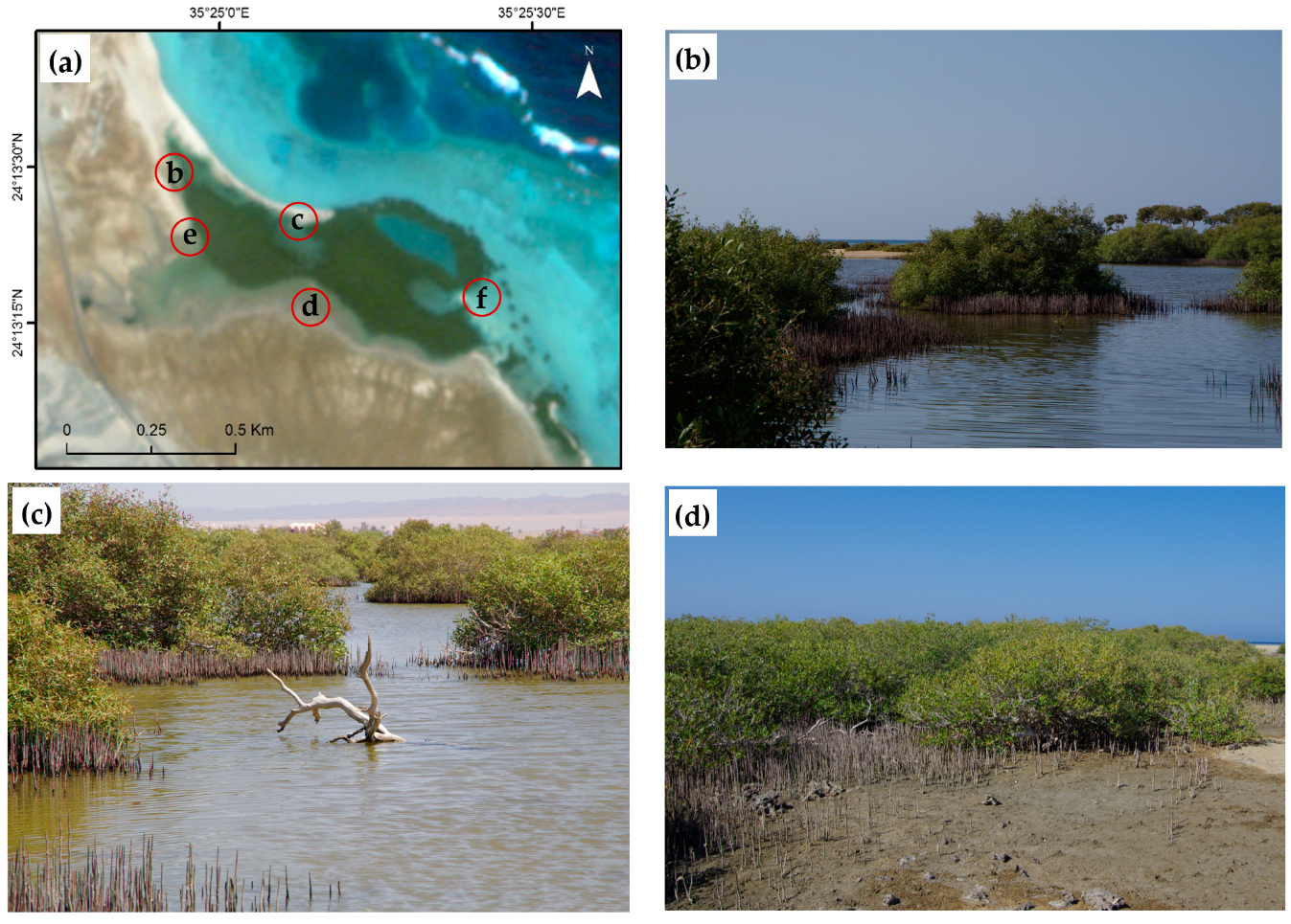
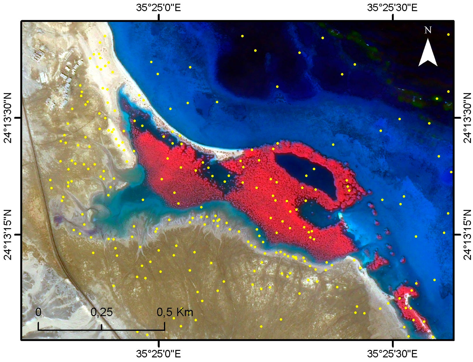
2.3. Field Data
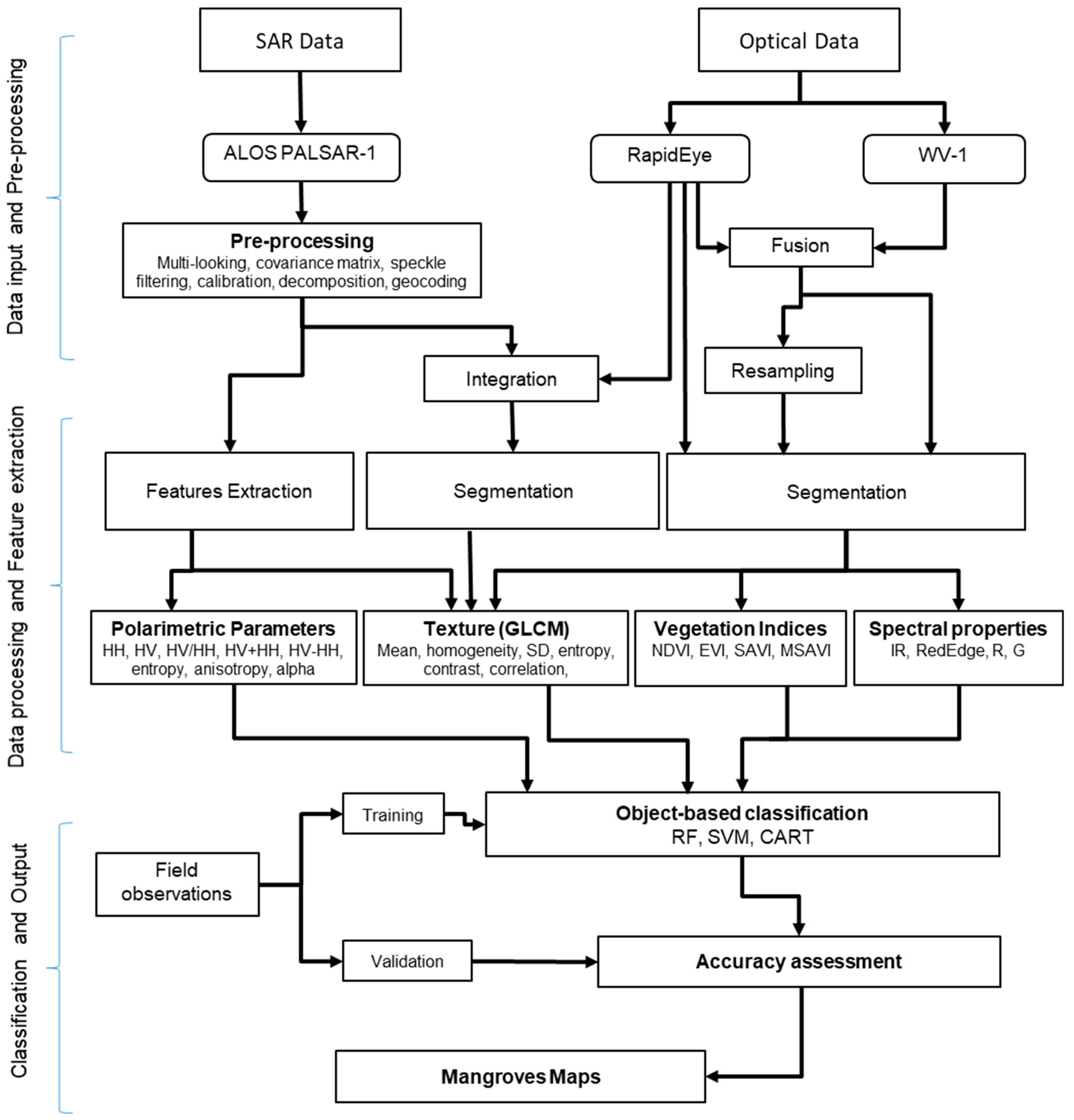
2.4. Object-Based Image Analysis and Feature Extraction
2.5. Image Classification
2.6. Accuracy Assessment
3. Results
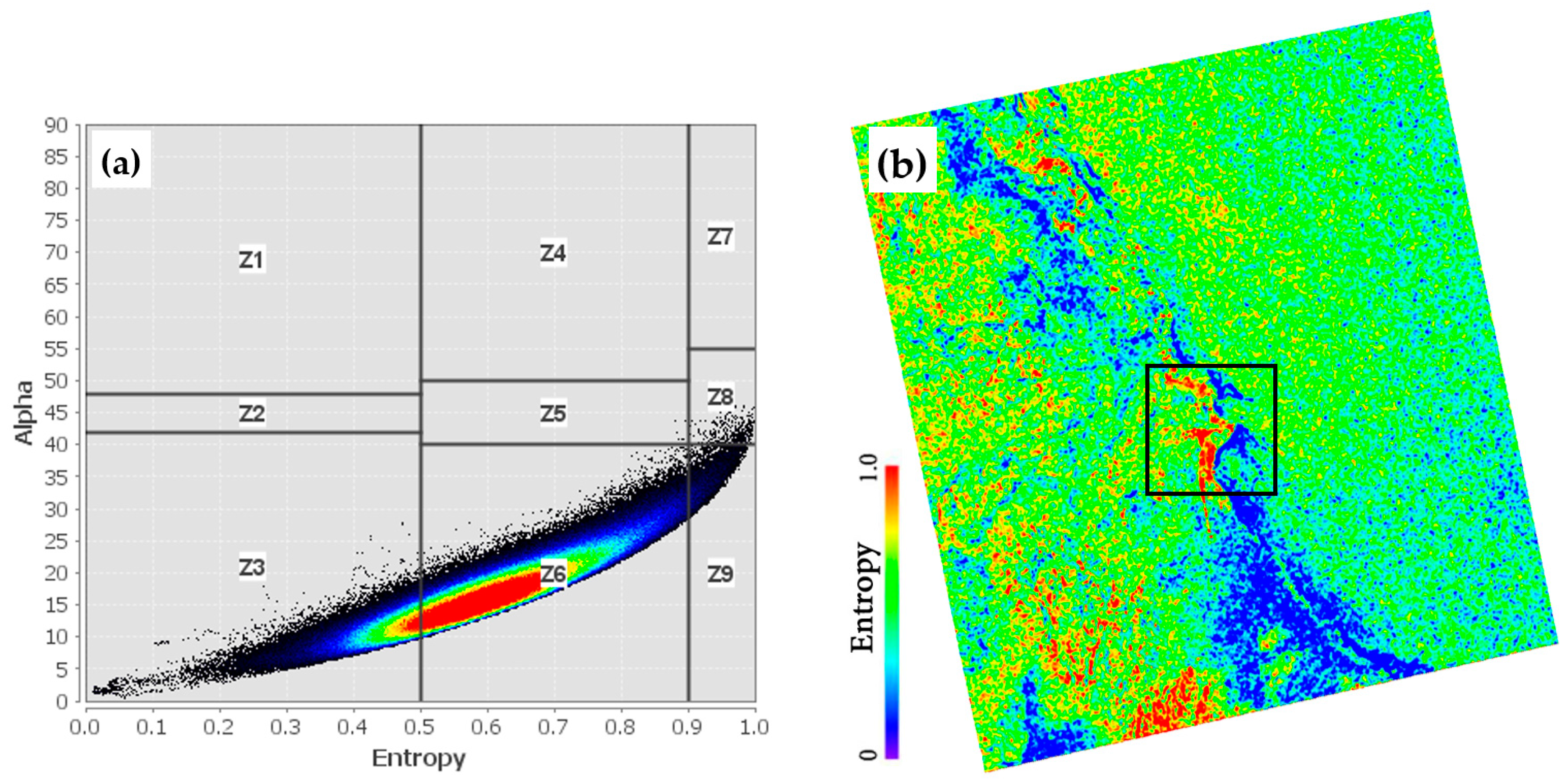
3.1. Backscattering Characterization and Polarimetric Parameters Description
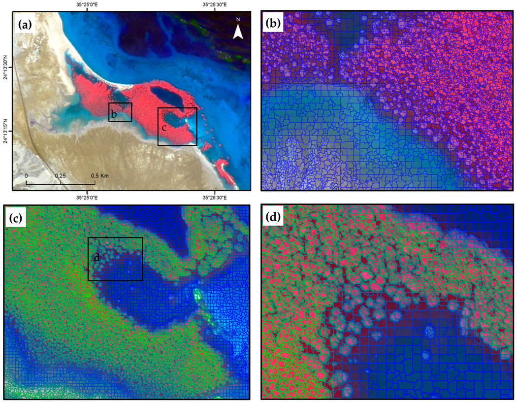
3.2. Segmentation and Feature Extraction
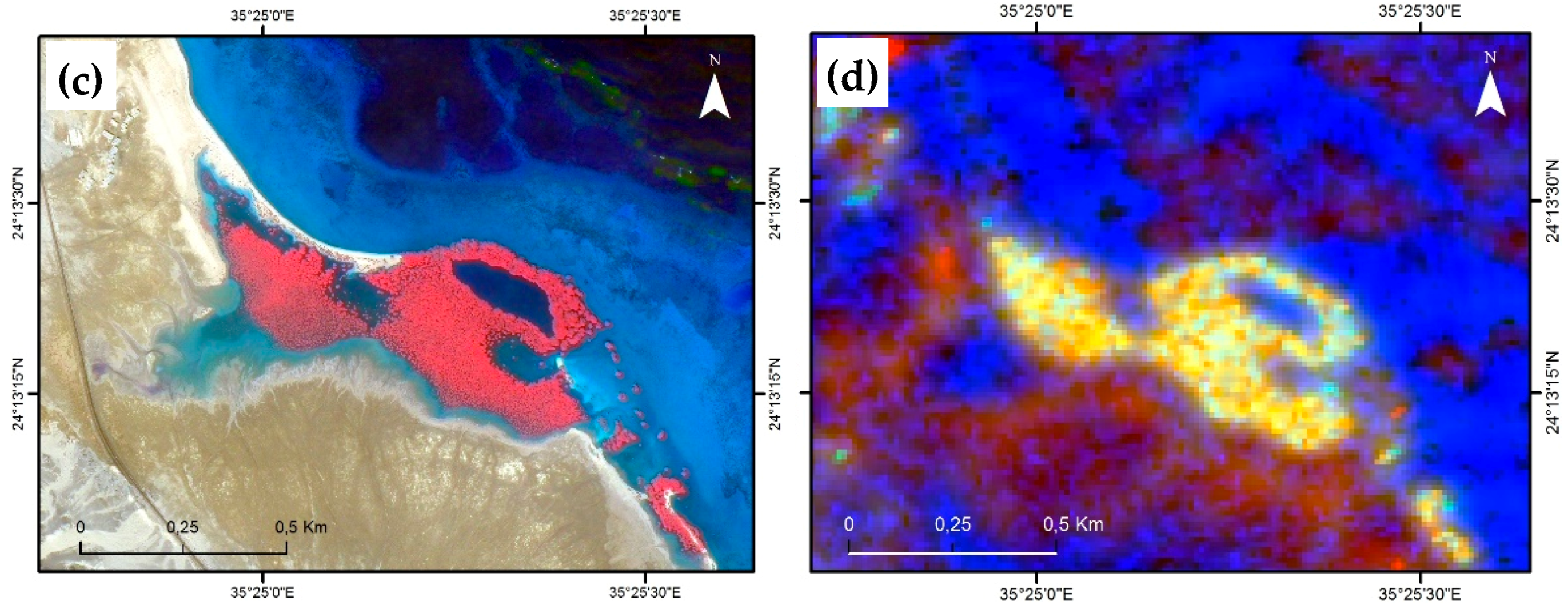
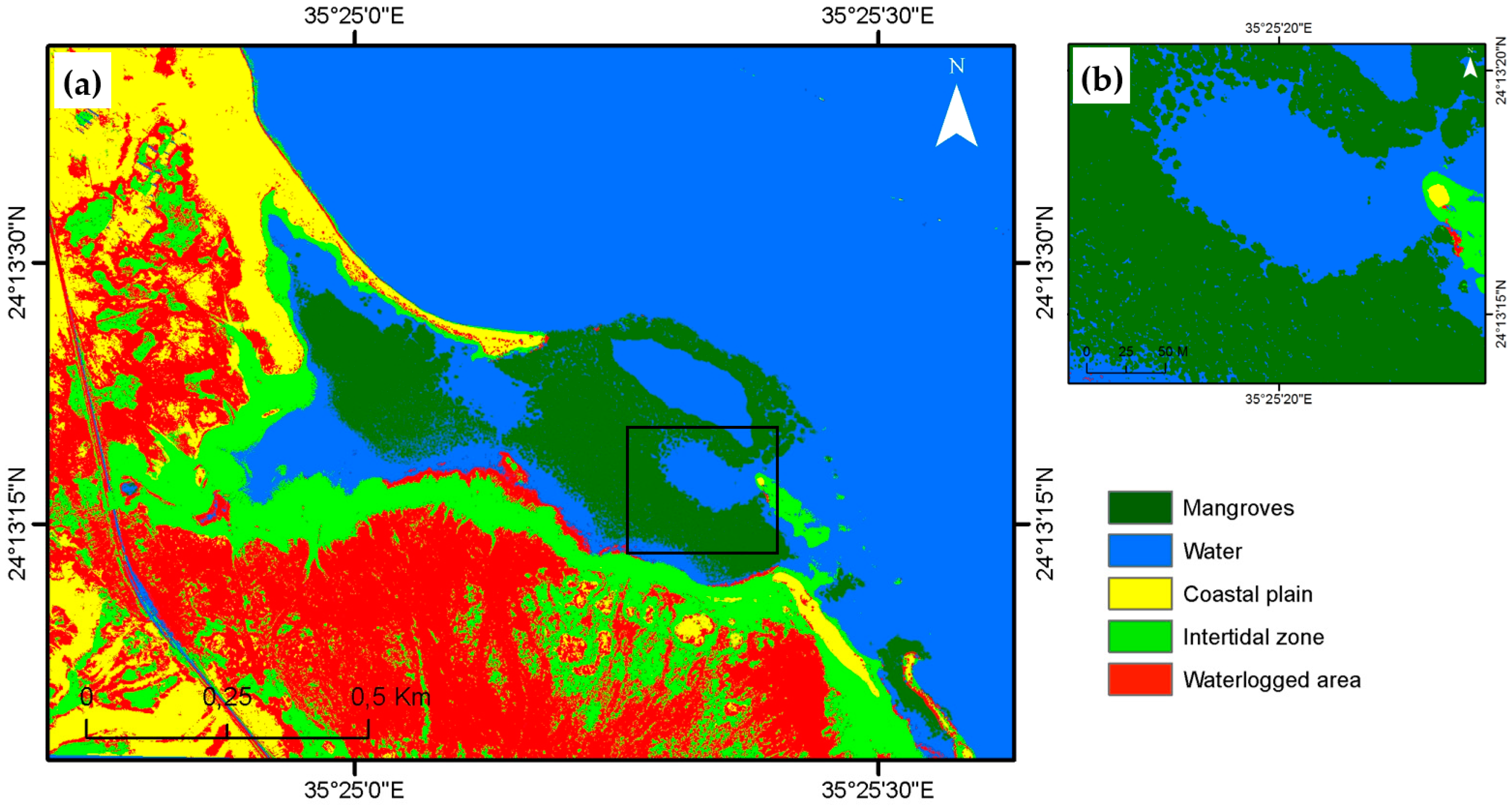
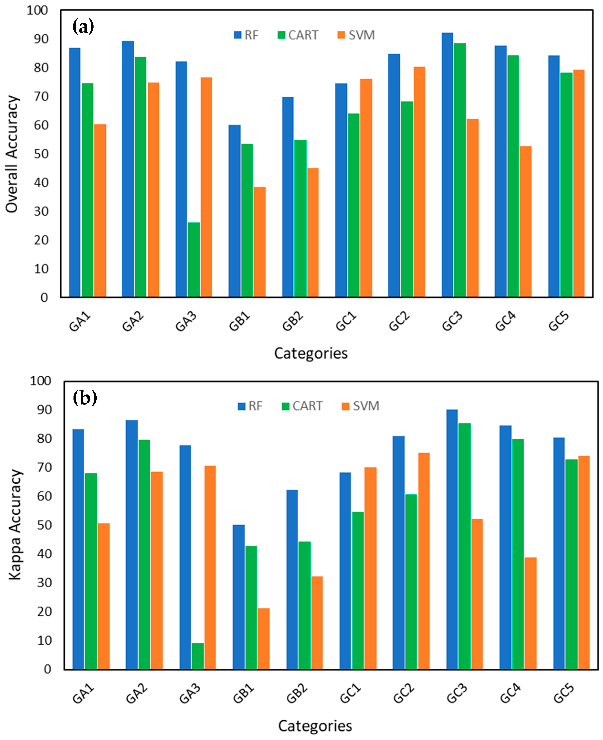
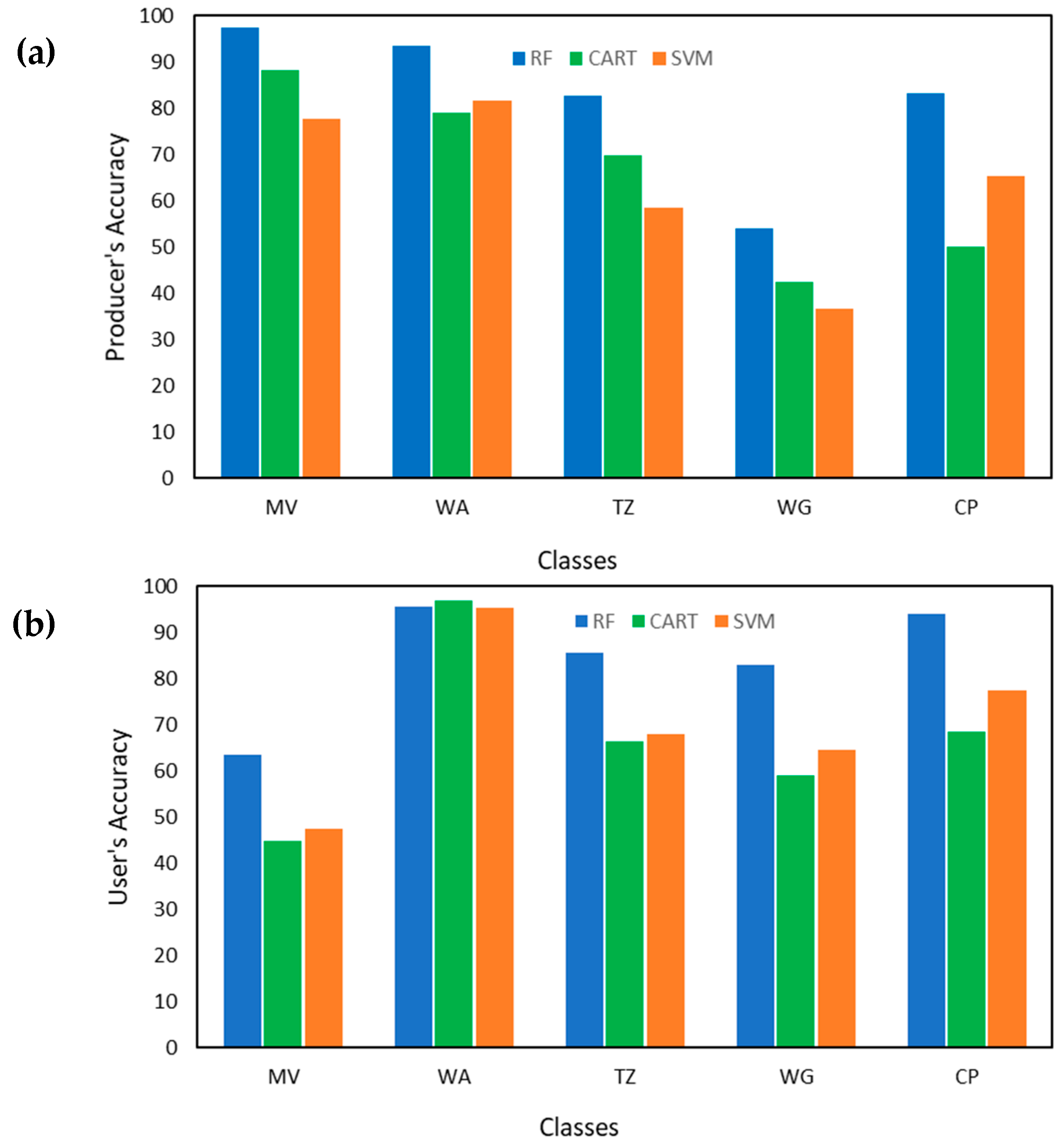
3.3. Classisifcation Results and Accuracy Assessment
4. Discussion
5. Conclusions
Acknowledgments
Author Contributions
Conflicts of Interest
References
- Spalding, M.D.; Blasco, F.; Field, C.D. World Mangrove Atlas; International Society for Mangrove Ecosystems: Okinawa, Japan, 1997. [Google Scholar]
- Barbier, E.B.; Sathiratai, S. Shrimp Farming and Mangrove Loss in Thailand; Edward Elgar: Cheltenham, UK, 2004. [Google Scholar]
- Giri, C.; Pengra, B.; Zhu, Z.; Singh, A.; Tieszen, L.L. Monitoring Mangrove forest dynamics of the Sundarbans in Bangladesh and India using multi-temporal satellite data from 1973 to 2000. Estuar. Coast. Shelf Sci. 2007, 73, 91–100. [Google Scholar] [CrossRef]
- Gedan, K.B.; Kirwan, M.L.; Wolanski, E.; Barbier, E.B.; Silliman, B.R. The present and future role of coastal wetland vegetation in protecting shorelines: Answering recent challenges to the paradigm. Clim. Chang. 2011, 106, 7–29. [Google Scholar] [CrossRef]
- Vo, Q.T.; Oppelt, N.; Leinenkugel, P.; Kuenzer, C. Remote sensing in mapping mangrove ecosystems—An object-based approach. Remote Sens. 2013, 5, 183–201. [Google Scholar] [CrossRef] [Green Version]
- Walters, B.B.; Roennbaeck, P.; Kovacs, J.; Crona, B.; Hussain, S.; Badola, R.; Primavera, J.H.; Barbier, E.B.; Dahdouh-Guebas, F. Ethnobiology, socio-economics and adaptive management of mangroves: A review. Aquat. Bot. 2008, 89, 220–236. [Google Scholar] [CrossRef]
- Beaumont, L.J.; Pitman, A.; Perkins, S.; Zimmermann, N.E.; Yoccoz, N.G.; Thuiller, W. Impacts of climate change on the world’s most exceptional ecoregions. Proc. Natl. Acad. Sci. USA 2011, 108, 2306–2311. [Google Scholar] [CrossRef] [PubMed]
- Feller, I.C.; Lovelock, C.E.; Berger, U.; McKee, K.L.; Joye, S.B.; Ball, M.C. Biocomplexity in mangrove ecosystems. Annu. Rev. Mar. Sci. 2010, 2, 395–417. [Google Scholar] [CrossRef] [PubMed]
- FAO. The World’s Mangroves 1980–2005; FAO Forestry 153; FAO: Rome, Italy, 2007. [Google Scholar]
- Lacerda, L.D. (Ed.) American mangroves. In Mangrove Ecosystems; Springer-Verlag: Berlin/Heidelberg, Germany, 2001; pp. 1–62. [Google Scholar]
- Hogarth, P.J. The Biology of Mangroves; Oxford University Press: Oxford, UK, 1999. [Google Scholar]
- Gilman, E.; Ellison, J.; Duke, N.C.; Field, C. Threats to mangroves from climate change and adaptation options: A review. Aquat. Bot. 2008, 89, 237–250. [Google Scholar] [CrossRef]
- Ellison, J.C. Vulnerability assessment of mangroves to climate change and sea-level rise impacts. Wetl. Ecol. Manag. 2015, 23, 115. [Google Scholar] [CrossRef]
- Galal, N. Studies on the Coastal Ecology and Management of the Nabq Protected Area, South Sinai, Egypt. Ph.D. Thesis, University of York, York, UK, 1999. [Google Scholar]
- Archibald, S.; Scholes, R.J. Leaf green-up in a semi-arid African savanna—Separating tree and grass responses to environmental cues. J. Veg. Sci. 2007, 181, 583–594. [Google Scholar]
- Held, A.; Ticehurst, C.; Lymburner, L.; Williams, N. High resolution mapping of tropical mangrove ecosystems using hyperspectral and radar remote sensing. Int. J. Remote Sens. 2003, 24, 2739–2759. [Google Scholar] [CrossRef]
- Green, E.P.; Mumby, P.J.; Edwards, A.J.; Clark, C.D. A review of remote sensing for the assessment and management of tropical coastal resources. Coast. Manag. 1996, 24, 1–40. [Google Scholar] [CrossRef]
- Jensen, J.R.; Lin, H.; Yang, X.; Ramsey, E.; Davis, B.A.; Thoemke, C.W. The measurement of mangrove characteristics in southwest Florida using SPOT multispectral data. Geochem. Int. 1991, 2, 13–21. [Google Scholar] [CrossRef]
- Rasolofoharinoro, M.; Blasco, F.; Bellan, M.; Aizpuru, M.; Gauquelin, T.; Denis, J. A remote sensing based methodology for mangrove studies in Madagascar. Int. J. Remote Sens. 1998, 19, 1873–1886. [Google Scholar] [CrossRef]
- Green, E.P.; Clark, C.D.; Mumby, P.J.; Edwards, A.J.; Ellis, A. Remote sensing techniques for mangrove mapping. Int. J. Remote Sens. 1998, 19, 935–956. [Google Scholar] [CrossRef]
- Long, B.G.; Skewes, T.D. A technique for mapping mangroves with Landsat TM satellite data and geographic information system. Estuar. Coast. Shelf Sci. 1996, 43, 373–381. [Google Scholar] [CrossRef]
- Neukermans, G.; Dahdouh-Guebas, F.; Kairo, J.G.; Koedam, N. Mangrove species and stand mapping in Gazi Bay (Kenya) using Quickbird satellite imagery. J. Spat. Sci. 2008, 53, 75–86. [Google Scholar] [CrossRef]
- Blaschke, T. Object based image analysis for remote sensing. ISPRS J. Photogramm. Remote Sens. 2010, 65, 2–16. [Google Scholar] [CrossRef]
- Ke, Y.; Quackenbush, L.J.; Im, J. Synergistic use of QuickBird multispectral imagery and LIDAR data for object-based forest species classification. Remote Sens. Environ. 2010, 114, 1141–1154. [Google Scholar] [CrossRef]
- Hay, G.J.; Castilla, G. Geographic Object-Based Image Analysis (GEOBIA): A new name for a new discipline. In Object Based Image Analysis; Blaschke, T., Lang, S., Hay, G., Eds.; Springer: Heidelberg/Berlin, Germany; New York, NY, USA, 2008; pp. 93–112. [Google Scholar]
- Liu, Y.; Li, M.; Mao, L.; Xu, F. Review of remotely sensed imagery classification patterns based on object oriented image analysis. Chin. Geogr. Sci. 2006, 16, 282–288. [Google Scholar] [CrossRef]
- Almeida-Filho, R.; Shimabukuro, Y.E.; Rosenqvist, A.; Sanchez, G.A. Using dual-polarized ALOS PALSAR data for detecting new fronts of deforestation in the Brazilian Amazonia. Int. J. Remote Sens. 2009, 30, 3735–3743. [Google Scholar] [CrossRef]
- Hoekman, D.H.; Vissers, M.A.M.; Wielaard, N. PALSAR wide-area mapping of Borneo: Methodology and map validation. IEEE J. Sel. Top. Appl. Earth Obs. Remote Sens. 2010, 3, 605–617. [Google Scholar] [CrossRef]
- Häme, T.; Rauste, Y.; Sirro, L.; Stach, N. Forest cover mapping in French Guiana since 1992 using satellite radar imagery. In Proceedings of the International Symposium on Remote Sensing of Environment (ISRSE 33), Stresa, Italy, 4–8 May 2009. [Google Scholar]
- Le Toan, T.; Quegan, S.; Davidson, M.W.J.; Balzter, H.; Paillou, P.; Papathanassiou, K.; Plummer, S.; Rocca, F.; Saatchi, S.; Shugart, H.; et al. The BIOMASS mission: Mapping global forest biomass to better understand the terrestrial carbon cycle. Remote Sens. Environ. 2011, 115, 2850–2860. [Google Scholar] [CrossRef]
- Sun, G.; Ranson, K.J.; Guo, Z.; Zhang, Z.; Montesano, P.; Kimes, D. Forest Biomass Mapping from Lidar and Radar Synergies. Remote Sens. Environ. 2011, 115, 2906–2916. [Google Scholar] [CrossRef]
- Santoro, M.; Shvidenko, A.; McCallum, I.; Askne, J.; Schmullius, C. Properties of ERS-1/2 coherence in the Siberian boreal forest and implications for stem volume retrieval. Remote Sens. Environ. 2007, 106, 154–172. [Google Scholar] [CrossRef]
- Carreiras, J.M.B.; Melo, J.B.; Vasconcelos, M.J. Estimating the above-ground biomass in Miombo Savanna Woodlands (Mozambique, East Africa) using L-band synthetic aperture radar data. Remote Sens. 2013, 5, 1524–1548. [Google Scholar] [CrossRef]
- Naidoo, L.; Mathieu, R.; Main, R.; Kleynhans, W.; Wessels, K.; Asner, G.; Leblon, B. Savannah woody structure modelling and mapping using multi-frequency (X-, C- and L-band) Synthetic Aperture Radar data. ISPRS J. Photogramm. Remote Sens. 2015, 105, 234–250. [Google Scholar] [CrossRef]
- Mitchard, E.T.A.; Saatchi, S.S.; Lewis, S.L.; Feldpausch, T.R.; Woodhouse, I.H.; Sonke, B.; Rowland, C.; Meir, P. Measuring biomass changes due to woody encroachment and deforestation/degradation in a forest-savanna boundary region of central Africa using multi-temporal L-band radar backscatter. Remote Sens. Environ. 2011, 115, 2861–2873. [Google Scholar] [CrossRef]
- Lucas, R.M.; Mitchell, A.L.; Rosenqvist, A.; Proisy, C.; Melius, A.; Ticehurst, C. The potential of L-band SAR for quantifying mangrove characteristics and change: Case studies from the tropics. Aquat. Conserv. Mar. Freshw. Ecosyst. 2007, 17, 245–264. [Google Scholar] [CrossRef]
- Aslan, A.; Abdullah, F.R.; Matthew, W.W.; Scott, M.R. Mapping spatial distribution and biomass of coastal wetland vegetation in Indonesian Papua by combining active and passive remotely sensed data. Remote Sens. Environ. 2016, 183, 65–81. [Google Scholar] [CrossRef]
- Zahran, M.A.; Willis, A.J. The Vegetation of Egypt, 2nd ed.; Chapman & Hall: London, UK, 2009; 424p. [Google Scholar]
- Tyc, G.; Tulip, J.; Schulten, D.; Krischke, M.; Oxfort, M. The RapidEye mission. Des. Acta Astronaut. 2005, 56, 213–219. [Google Scholar] [CrossRef]
- Wegmüller, U. Automated terrain corrected SAR geocoding. In Proceedings of the IGARSS 1999, Hamburg, Germany, 28 June–2 July 1999. [Google Scholar]
- Santini, N.S.; Hua, Q.; Schmitz, N.; Lovelock, C.E. Radiocarbon Dating and Wood Density Chronologies of Mangrove Trees in Arid Western Australia. PLoS ONE 2013, 8, e80116. [Google Scholar] [CrossRef] [PubMed]
- Shimada, M.; Isoguchi, O.; Tadono, T.; Isono, K. PALSAR radiometric and geometric calibration. IEEE Trans. Geosci. Remote Sens. 2009, 47, 3915–3932. [Google Scholar] [CrossRef]
- Maurizio, S.; Eriksson, L.E.B.; Fransson, J.E.S. Reviewing ALOS PALSAR backscatter observations for stem volume retrieval in Swedish forest. Remote Sens. 2015, 7, 4290–4317. [Google Scholar] [CrossRef]
- Lee, J.S.; Grunes, M.R.; de Grandi, G. Polarimetric SAR speckle filtering and its implication for classification. IEEE Trans. Geosci. Remote Sens. 1999, 37, 2363–2373. [Google Scholar]
- Cloude, S.R.; Pottier, E. An entropy based classification scheme for land applications of polarimetric SAR. IEEE Trans. Geosci. Remote Sens. 1997, 35, 68–78. [Google Scholar] [CrossRef]
- Pottier, E.; Ferro-Famil, L.; Allain, S.; Cloude, S.; Hajnsek, I.; Papathanassiou, K.; Moreira, A.; Williams, M.; Minchella, A.; Lavalle, M.; et al. Overview of the PolSARpro V4.0 software: The open source toolbox for polarimetric and interferometric polarimetric SAR data processing. In Proceedings of the IEEE International Geoscience and Remote Sensing Symposium, Cape Town, South Africa, 12–17 July 2009; pp. IV-936–IV-939. [Google Scholar]
- Treuhaft, R.N.; Law, B.E.; Asner, G.P. Forest attributes from radar interferometric structure and its fusion with optical remote sensing. Bioscience 2004, 54, 561–571. [Google Scholar] [CrossRef]
- Amarsaikhana, D.; Blotevogelb, H.H.; van Genderenc, J.L.; Ganzoriga, M.; Gantuyaa, R.; Nerguia, B. Fusing high-resolution SAR and optical imagery for improved urban land cover study and classification. Int. J. Image Data Fusion 2010, 1, 83–97. [Google Scholar] [CrossRef]
- Pohl, C.; Van Genderen, J.L. Multisensor image fusion in remote sensing: Concepts, methods and applications. Int. J. Remote Sens. 1998, 19, 823–854. [Google Scholar] [CrossRef]
- Ehlers, M.; Klonus, S.; Johan, Ã.; Strand, P.R.; Rosso, P. Multi-sensor image fusion for pan-sharpening in remote sensing. Int. J. Image Data Fusion 2010, 1, 25–45. [Google Scholar] [CrossRef]
- Lang, S. Object-based image analysis for remote sensing applications: Modeling reality—Dealing with complexity. In Object-Based Image Analysis; Blaschke, T., Lang, S., Hay, G.J., Eds.; Springer: Heidelberg/Berlin, Germany; New York, NY, USA, 2008; pp. 1–25. [Google Scholar]
- Benz, U.C.; Hofmann, P.; Willhauck, G.; Lingenfelder, I.; Heynen, M. Multi-resolution, object-oriented fuzzy analysis of remote sensing data for GIS-ready information. ISPRS J. Photogramm. Remote Sens. 2004, 58, 239–258. [Google Scholar] [CrossRef]
- Baatz, M.; Schäpe, A. Multiresolution Segmentation—An optimization approach for high quality multi-scale image segmentation. In Angewandte Geographische Informationsverarbeitung XII; Strobl, J., Blaschke, T., Griesebner, G., Eds.; Wichmann: Heidelberg, Germany, 2000; pp. 12–23. [Google Scholar]
- Xiaoxiao, L.; Soe, W.M.; Yujia, Z.; Chritopher, G.; Xiaoxiang, Z.; Billie, L.T. Object-based land cover classification for metropolitan Phoenix, Arizona, using aerial photography. Int. J. Appl. Earth Obs. Geoinf. 2014, 33, 321–330. [Google Scholar]
- Definiens. Ecognition. 2009. Available online: http://www.ecognition.com (accessed on 10 June 2015).
- Laliberte, A.S.; Fredrickson, E.L.; Rango, A. Combining decision trees with hierarchical object-oriented image analysis for mapping arid rangelands. Photogramm. Eng. Remote Sens. 2007, 73, 197–207. [Google Scholar] [CrossRef]
- Marceau, D. The scale issue in the social and natural sciences. Can. J. Remote Sens. 1999, 25, 347–356. [Google Scholar] [CrossRef]
- Münch, Z.; Okoye, P.I.; Gibson, L.; Mantel, S.; Palmer, A. Characterizing Degradation Gradients through Land Cover Change Analysis in Rural Eastern Cape, South Africa. Geosciences 2017, 7, 7. [Google Scholar] [CrossRef]
- Taylor, P.J. Quantitative Methods in Geography: An Introduction to Spatial Analysis; Houghton Mifflin Boston: Boston, MA, USA, 1977. [Google Scholar]
- Haralick, R.M.; Shanmugam, K.; Dinstein, I. Textural features for image classification. IEEE Trans. Syst. Man Cybern 1973, 6, 269–285. [Google Scholar] [CrossRef]
- Hurni, K.; Hett, C.; Epprecht, M.; Messerli, P.; Heinimann, A. A texture-based land cover classification for the delineation of a shifting cultivation landscape in the Lao PDR using landscape metrics. Remote Sens. 2013, 5, 3377–3396. [Google Scholar] [CrossRef] [Green Version]
- Carlson, T.N.; Ripley, D.A. On the relation between NDVI, fractional vegetation cover, and Leaf Area Index. Remote Sens. Environ. 1997, 62, 241–252. [Google Scholar] [CrossRef]
- Wang, Z.; Liu, C.; Huete, A. From AVHRR-NDVI to MODIS-EVI: Advances in vegetation index research. Acta Ecol. Sin. 2002, 23, 979–987. [Google Scholar]
- Huete, A.; Didan, K.; Miura, T.; Rodriguez, E.P.; Gao, X.; Ferreira, L.G. Overview of the radiometric and biophysical performance of the MODIS vegetation indices. Remote Sens. Environ. 2002, 83, 195–213. [Google Scholar] [CrossRef]
- Haboudane, D.; Miller, J.R.; Pattey, E.; Zarco-Tejada, P.J.; Strachan, I.B. Hyperspectral vegetation indices and novel algorithms for predicting green LAI of crop canopies: Modelling and validation in the context of precision agriculture. Remote Sens. Environ. 2004, 90, 337–352. [Google Scholar] [CrossRef]
- Kauth, R.J.; Thomas, G.S. The tasseled cap-A graphic description of the spectral-temporal development of agricultural crops as seen by Landsat. In Proceedings of the Symposium on Machine Processing of Remotely Sensed Data, West Lafayette, IN, USA, 9 June–1 July 1976; pp. 4B-41–4B-50. [Google Scholar]
- Schönert, M.; Weichelt, H.; Zillmann, E.; Jürgens, C. Derivation of tasseled cap coefficients for RapidEye data. In Proceedings of the SPIE 9245, Earth Resources and Environmental Remote Sensing/GIS Applications V, Amsterdam, The Netherlands, 23–25 September 2014; p. 92450Q. [Google Scholar] [CrossRef]
- Dorigo, W.; Lucieer, A.; Podobnikar, T.; Carni, A. Mapping invasive Fallopia japonica by combined spectral, spatial, and temporal analysis of digital orthophotos. Int. J. Appl. Earth Obs. Geoinf. 2012, 19, 185–195. [Google Scholar] [CrossRef]
- Lu, D.; Batistella, M. Exploring TM image texture and its relationships with biomass estimation in Rondônia, Brazilian Amazon. Acta Amaz. 2005, 35, 249–257. [Google Scholar] [CrossRef]
- Tucker, C.J. Red and Photographic Infrared Linear Combinations for Monitoring Vegetation. Remote Sens. Environ. 1979, 8, 127–150. [Google Scholar] [CrossRef]
- Gitelson, A.; Kaufman, Y.; Merzlyak, M. Use of a green channel in remote sensing of global vegetation from EOS-MODIS. Remote Sens. Environ. 1996, 58, 289–298. [Google Scholar] [CrossRef]
- Jiang, Z.; Huete, A.R.; Didan, K.; Miura, T. Development of a two-band enhanced vegetation index without a blue band. Remote Sens. Environ. 2008, 112, 3833–3845. [Google Scholar] [CrossRef]
- Huete, A.R. A soil-adjusted vegetation index (SAVI). Remote Sens. Environ. 1988, 25, 295–309. [Google Scholar] [CrossRef]
- Qi, J.; Chehbouni, A.; Huete, A.R.; Kerr, Y.H.; Sorooshian, S. A Modified Soil Adjusted Vegetation Index. Remote Sens. Environ. 1994, 48, 119–126. [Google Scholar] [CrossRef]
- Gislason, P.O.; Benediktsson, J.A.; Sveinsson, J.R. Random forests for land cover classification. Pattern Recogn. Lett. 2006, 27, 294–300. [Google Scholar] [CrossRef]
- Vapnik, V. Estimation of Dependences Based on Empirical Data; Springer Series in Statistics; Springer: Secaucus, NJ, USA, 1982. [Google Scholar]
- Foody, G.M.; Mathur, A. Toward intelligent training of supervised image classifications: Directing training data acquisition for SVM classification. Remote Sens. Environ. 2004, 93, 107. [Google Scholar] [CrossRef]
- Van Der Linden, S.; Hostert, P. The influence of urban structures on impervious surface maps from airborne hyperspectral data. Remote Sens. Environ. 2009, 113, 2298–2305. [Google Scholar] [CrossRef]
- Meyer, D. Support Vector Machines. 2014. Available online: http://cran.rproject.org/web/packages/e1071/vignettes/svm-doc.pdf (accessed on 27 February 2018).
- Friedl, M.A.; Brodley, C.E. Decision tree classification of land cover from remotely sensed data. Remote Sens. Environ. 1997, 61, 399–409. [Google Scholar] [CrossRef]
- Hansen, M.; Dubayah, R.; Defries, R. Classification trees: An alternative to traditional land cover classifiers. Int. J. Remote Sens. 1996, 17, 1075–1081. [Google Scholar] [CrossRef]
- Lawrence, R.L.; Wright, A. Rule-based classification systems using classification and regression tree (CART) analysis. Photogramm. Eng. Remote Sens. 2001, 67, 1137–1142. [Google Scholar]
- Foody, G.M. Status of Land Cover Classification Accuracy Assessment. Remote Sens. Environ. 2002, 80, 185–201. [Google Scholar] [CrossRef]
- Rogan, J.; Miller, J.; Stow, D.; Franklin, J.; Levien, L.; Fisher, C. Land-cover change monitoring with classification trees using Landsat TM and ancillary data. Photogramm. Eng. Remote Sens. 2003, 69, 793–804. [Google Scholar] [CrossRef]
- McCoy, R.M. Field Methods in Remote Sensing; Guildford Press: New York, NY, USA, 2005. [Google Scholar]
- Congalton, R.G.; Green, K. Assessing the Accuracy of Remotely Sensed Data: Principles and Practices; Lewis Publishers: Boca Raton, FL, USA, 1999. [Google Scholar]
- Haack, B.; Bechdol, M. Integrating multisensor data and RADAR texture measures for land cover mapping. Comput. Geosci. 2000, 26, 411–421. [Google Scholar] [CrossRef]
- Laurin, G.V.; Liesenberg, V.; Chen, Q.; Guerriero, L.; Frate, F.D.; Bartolini, A.; Coomes, D.; Wilebore, B.; Lindsell, J.; Valentini, R. Optical and SAR sensor synergies for forest and land cover mapping in a tropical site in West Africa. Int. J. Appl. Earth Obs. Geoinf. 2013, 21, 7–16. [Google Scholar] [CrossRef]
- Lang, M.; McCarty, G. Wetland Mapping: History and Trends. In Wetlands: Ecology, Conservation and Management; Russo, R.E., Ed.; Nova Publishers: New York, NY, USA, 2008; pp. 74–112. [Google Scholar]
- Ramsey, E.W., III; Chappell, D.K.; Jacobs, D.; Sapkota, S.K.; Baldwin, D.G. Resource management of forested wetlands: Hurricane impact and recovery mapping by combining Landsat TM and NOAA AVHRR data. Photogramm. Eng. Remote Sens. 1998, 64, 733–738. [Google Scholar]
- Waleska, S.; Rodrigues, P.; Walfir, P.; Souza-Filho, M. Use of Multi-Sensor Data to Identify and Map Tropical Coastal Wetlands in the Amazon of Northern Brazil. Wetlands 2011, 31, 11–23. [Google Scholar]
- Ghosh, A.; Fassnacht, F.E.; Joshi, P.K.; Koch, B. A framework for mapping tree species combining hyperspectral and LiDAR data: Role of selected classifiers and sensor across three spatial scales. Int. J. Appl. Erath Obs. Geoinf. 2014, 26, 49–63. [Google Scholar] [CrossRef]
- Burai, P.; Deak, B.; Valko, O.; Tomor, T. Classification of herbaceous vegetation using airborne hyperspectral imagery. Remote Sens. 2014, 7, 2046–2066. [Google Scholar] [CrossRef]
- Ismail, R.; Mutanga, O.; Kumar, L. Modelling the potential distribution of pine forests susceptible to Sirex Noctilo infestations in Mpumalanga, South Africa. Trans. GIS 2010, 14, 709–726. [Google Scholar] [CrossRef]
- Prasad, A.M.; Iverson, L.R.; Liaw, A. Newer classification and regression tree techniques: Bagging and random forests for ecological prediction. Ecosystems 2006, 9, 181–199. [Google Scholar] [CrossRef]
- Anguita, D.; Ghio, A.; Greco, N.; Oneto, L.; Ridella, S. Model Selection for Support Vector Machines: Advantages and Disadvantages of the Machine Learning Theory. In Proceedings of the International Joint Conference on Neural Networks, Barcelona, Spain, 18–23 July 2010; pp. 1–8. [Google Scholar]
- Wang, L.; Silván-Cárdenas, J.L.; Sousa, W.P. Neural Network Classification of Mangrove Species from Multi-seasonal Ikonos Imagery. Photogram. Eng. Remote Sens. 2008, 74, 921–927. [Google Scholar] [CrossRef]
- Kamal, M.; Phinn, S.; Johansen, K. Object-Based Approach for Multi-Scale Mangrove Composition Mapping Using Multi-Resolution Image Datasets. Remote Sens. 2015, 7, 4753–4783. [Google Scholar] [CrossRef]
- Longepe, N.; Rakwatin, P.; Isoguchi, O.; Shimada, M.; Uryu, Y.; Yulianto, K. Assessment of ALOS PALSAR 50 m orthorectified FBD data for regional land cover classification by support vector machines. IEEE Trans. Geosci. Remote Sens. 2011, 49, 2135–2150. [Google Scholar] [CrossRef]
- Wang, L.; Sousa, W.P.; Gong, P.; Biging, G.S. Comparison of IKONOS and QuickBird images for mapping mangrove species on the Caribbean coast of Panama. Remote Sens. Environ. 2004, 91, 432–440. [Google Scholar] [CrossRef]
- Hess, L.L.; Melack, J.M.; Filoso, S.; Wang, Y. Delineation of inundated area and vegetation along the Amazon floodplain with the SIR-C synthetic aperture radar. IEEE Trans. Geosci. Remote Sens. 1995, 33, 896–904. [Google Scholar] [CrossRef]
- Bourgeau-Chavez, L.L.; Riordan, K.; Powell, R.B.; Miller, N.; Nowels, M. Improving wetland characterization with multi-sensor, multi-temporal SAR and optical/infrared data fusion. In Advances in Geoscience and Remote Sensing; Jedlovec, G., Ed.; InTech: Rijeka, Croatia, 2009. [Google Scholar]
- Souza-Filho, P.W.M.; Paradella, W.R.; Rodrigues, S.W.P.; Costa, F.R.; Mura, J.C.; Gonçalves, F.D. Discrimination of coastal wetland environments in the Amazon region based on multi-polarized L-band airborne Synthetic Aperture Radar imagery. Estuar. Coast. Shelf Sci. 2011, 95, 88–98. [Google Scholar] [CrossRef]


| Categories | Variables | Algorithm | Reference |
|---|---|---|---|
| VIs | NDVI | [70] | |
| gNDVI | [71] | ||
| EVI2 | [72] | ||
| SAVI | [73] | ||
| MSAVI | [74] | ||
| GLCM texture | MEN | [60] | |
| VAR | |||
| HOM | |||
| CON | |||
| ENT | |||
| DIS | |||
| COR | |||
| SEC |
| Category | Datasets | Selected Features and Combinations | |
|---|---|---|---|
| GA | GA1 | Spectral bands | B, G, R, Red Edge, and NIR |
| GA2 | Spectral bands, VIs, and PCA | B, G, R, Red Edge, NIR, VIs, pc1, and pc2 | |
| GA3 | Spectral bands, VIs, PCA, and texture | B, G, R, Red Edge, NIR, VIs, pc1, pc2, and texture | |
| GB | GB1 | SAR bands | HH and HV |
| GB2 | SAR bands, PolSAR parameters, and GLCM texture | HH, HV, HV/HH, HV + HH, HV − HH, H, A, α, and GLCM texture | |
| GC | GC1 | Spectral bands, and SAR bands | B, G, R, Red Edge, NIR, HH, and HV |
| GC2 | Spectral bands, VIs, SAR bands, and PolSAR parameters | B, G, R, Red Edge, NIR, VIs, HH, HV, HV/HH, HV + HH, HV − HH, H, A, and α | |
| GC3 | Spectral bands, SAR bands, and PolSAR parameters | B, G, R, Red Edge, NIR, HH, HV, HV/HH, HV + HH, HV − HH, H, A, and α | |
| GC4 | Spectral bands, VIs, and SAR bands | B, G, R, Red Edge, NIR, VIs, HH, and HV | |
| GC5 | Spectral bands, VIs, SAR bands, PolSAR parameters, and texture | B, G, R, Red Edge, NIR, VIs, HH, HV, HV/HH, HV + HH, HV − HH, H, A, α, and GLCM texture | |
| Class | HH Backscattering (dB) | HV Backscattering (dB) | ||||
|---|---|---|---|---|---|---|
| Range | Mean | SD | Range | Mean | SD | |
| WA | −26.54 to −18.59 | −23.66 | 2.15 | −29.40 to −25.96 | −28.04 | 1.07 |
| MV | −10.98 to −05.72 | −8.19 | 1.35 | −20.37 to −14.60 | −16.86 | 1.18 |
| TZ | −18.77 to −15.51 | −16.10 | 3.36 | −27.96 to −24.99 | −26.38 | 0.65 |
| WG | −18.67 to −15.30 | −17.15 | 1.14 | −28.81 to −26.68 | −27.77 | 0.55 |
| CP | −24.27 to −20.58 | −22.46 | 0.94 | −29.11 to −27.44 | −28.26 | 0.48 |
| Categories | Subgroups | Overall Accuracy (OA) % | Kappa Coefficient (K) % | ||||
|---|---|---|---|---|---|---|---|
| RF | CART | SVM | RF | CART | SVM | ||
| GA (Optical data) | GA1 | 86.78 | 74.42 | 60.33 | 83.44 | 68.14 | 50.73 |
| GA2 | 89.26 | 83.72 | 74.79 | 86.57 | 79.68 | 68.63 | |
| GA3 | 82.23 | 26.03 | 76.45 | 77.86 | 9.02 | 70.63 | |
| GB (SAR data) | GB1 | 59.92 | 53.31 | 38.43 | 50.15 | 42.71 | 21.19 |
| GB2 | 69.83 | 54.65 | 45.04 | 62.21 | 44.36 | 32.31 | |
| GC (Integrated optical and SAR data) | GC1 | 74.42 | 63.95 | 75.97 | 68.28 | 54.74 | 70.23 |
| GC2 | 84.71 | 68.18 | 80.23 | 80.89 | 60.62 | 75.29 | |
| GC3 | 92.15 | 88.43 | 62.02 | 90.18 | 85.53 | 52.32 | |
| GC4 | 87.60 | 84.11 | 52.71 | 84.55 | 80.04 | 38.83 | |
| GC5 | 84.30 | 78.10 | 79.25 | 80.42 | 72.78 | 74.04 | |
© 2018 by the authors. Licensee MDPI, Basel, Switzerland. This article is an open access article distributed under the terms and conditions of the Creative Commons Attribution (CC BY) license (http://creativecommons.org/licenses/by/4.0/).
Share and Cite
Abdel-Hamid, A.; Dubovyk, O.; Abou El-Magd, I.; Menz, G. Mapping Mangroves Extents on the Red Sea Coastline in Egypt using Polarimetric SAR and High Resolution Optical Remote Sensing Data. Sustainability 2018, 10, 646. https://doi.org/10.3390/su10030646
Abdel-Hamid A, Dubovyk O, Abou El-Magd I, Menz G. Mapping Mangroves Extents on the Red Sea Coastline in Egypt using Polarimetric SAR and High Resolution Optical Remote Sensing Data. Sustainability. 2018; 10(3):646. https://doi.org/10.3390/su10030646
Chicago/Turabian StyleAbdel-Hamid, Ayman, Olena Dubovyk, Islam Abou El-Magd, and Gunter Menz. 2018. "Mapping Mangroves Extents on the Red Sea Coastline in Egypt using Polarimetric SAR and High Resolution Optical Remote Sensing Data" Sustainability 10, no. 3: 646. https://doi.org/10.3390/su10030646