Achieving Highly Efficient Atmospheric CO2 Uptake by Artificial Upwelling
by
Yiwen Pan
1, 
Long You
1,
Yifan Li
1,
Wei Fan
2,*,
Chen-Tung Arthur Chen
1,3,
Bing-Jye Wang
3 and
Ying Chen
2 1
Department of Ocean Science, Zhejiang University, Zhoushan 316021, China
2
Department of Ocean Engineering, Zhejiang University, Zhoushan 316021, China
3
Department of Oceanography, National Sun Yat-sen University, Kaohsiung 804, Taiwan
*
Author to whom correspondence should be addressed.
Sustainability 2018, 10(3), 664; https://doi.org/10.3390/su10030664
Submission received: 18 December 2017
/
Revised: 20 February 2018
/
Accepted: 20 February 2018
/
Published: 1 March 2018
(This article belongs to the Special Issue Marine Carbon Cycles)
Abstract
:Artificial upwelling (AU) is considered a potential means of reducing the accumulation of anthropogenic CO2. It has been suggested that AU has significant effects on regional carbon sink or source characteristics, and these effects are strongly influenced by certain technical parameters, the applied region, and the season. In this study, we simulated the power needed to raise the level of deep ocean water (DOW) to designated plume trapping depths in order to evaluate the effect of changing the source DOW depth and the plume trapping depth on carbon sequestration ability and efficiency. A carbon sequestration efficiency index (CSEI) was defined to indicate the carbon sequestration efficiency per unit of power consumption. The results suggested that the CSEI and the carbon sequestration ability exhibit opposite patterns when the DOW depth is increased, indicating that, although raising a lower DOW level can enhance the regional carbon sequestration ability, it is not energy-efficient. Large variations in the CSEI were shown to be associated with different regions, seasons, and AU technical parameters. According to the simulated CSEI values, the northeast past of the Sea of Japan is most suitable for AU, and some regions in the South China Sea are not suitable for increasing carbon sink.
1. Introduction
The potential of artificial upwelling (AU) to counteract accumulation of anthropogenic CO2 has attracted increasing scientific and policy interest [1,2]. It is proposed that, for climatic benefit, the growth of phytoplankton could be stimulated by input of nutrient-rich deep ocean water (DOW) [3] and thus significantly increase the uptake of atmospheric CO2 by increasing the portion of organic carbon that sinks into the deep ocean via the biological pump [4]. However, changing the input of high dissolved inorganic carbon (DIC) DOW from cold and deep to warm and shallow directly enhances its CO2 fugacity (fCO2), which makes the role of AU in modulating the carbon cycle complex [5,6]. Model-based estimates of CO2 sequestration effects have been found highly variable and often negative [7,8,9] in terms of AU’s sequestration effects on atmospheric CO2. Under the most optimistic assumptions, a sequestration rate of approximately 0.9 PgC/yr [7] of atmospheric CO2 was reported to be possible under AU, although 80% of the 0.9 PgC/yr would be stored on land and only 20% in the ocean. An amount of less than 0.2 PgC/yr in the ocean is around seven percent of the CO2 uptake rate of the global open ocean and two percent of the anthropogenic CO2 emissions value [10]. Keller et al. (2014) observed similar carbon sequestration characteristics but doubted that the sequestration effect could counteract the anthropogenic emissions [8]. Yool et al. (2009), however, suggested a considerably smaller and even negative effect of AU on atmospheric CO2 uptake [9]. Several natural upwelling events have been reported as carbon sources, and several have been reported as carbon sinks at different locations or, occasionally, at the same location but in different seasons. The juxtaposition of strong sources and sinks for atmospheric CO2 has been observed in coastal zones off Oregon and Chile during upwelling events [11,12,13,14]. It can be concluded that, given the complex carbon cycle processes caused by upwelling, carbon sink or source characteristics of a regional sea must be controlled by a combination of biogeochemical factors, including nutrient concentration and composition of the source DOW, differences in the DIC, the TA, and the temperature between the surface and the source water.
In our previous paper, large variations in carbon sequestration ability were reported to be associated with regions, seasons, and AU technical settings. In some regions, the regional carbon sink/source status could be changed from sources to sinks, if an optimum plume could be formed, with proper technical settings being established [15]. Considering the size and residence time of oceanic carbon reservoirs, it is of great importance to investigate AU as a potential geoengineering scheme to reduce anthropogenic CO2, after establishing the correct conditions, including the region, the season, and the technical parameters, especially on a large scale.
The previous simulation results showed that a general increase in the pattern of the regional carbon sequestration potential of AU occurs when the source DOW depth is increased. However, raising a lower DOW level to the euphotic layer with longer pipes would inevitably increase the power consumption of AU [16,17], not to mention the exacerbation of challenges in designing, fabricating, and deploying a technologically robust AU with structural longevity [18]. In fact, although a range of AU systems based on different rising principles and power supplies has been proposed over the past several decades, few have been reported to be successful in raising DOW levels to the euphotic layer in sea trials, especially for long-term operations [3,19,20,21,22,23,24]. For a real application of AU, especially on a large scale, even if the difficulties and expenses in design, fabrication, deployment, and maintenance of a long-pipe AU system are disregarded, such an application should employ a DOW depth and a plume trapping depth that can achieve a sufficiently large carbon sequestration value while keeping the power consumption relatively low.
In this study, we define an index to indicate the carbon sequestration efficiency (CSEI) in terms of power consumption and simulate the CO2 uptake efficiency. The effects of changing the source DOW depth and discharging depth on the regional CO2 uptake ability and efficiency were investigated under the condition that other technical settings are adjusted to form an optimum plume in a designated sub-layer. The regional and seasonal effects on the regional CO2 uptake ability and efficiency were also evaluated. AU-induced carbon transformation simulation was carried out using observed carbon and nutrient data from 16 selected stations ranging from 12 to 43°N, and from 110 to 137°E. Five stations in the ECS that were determined as inappropriate for applying AU to sequester atmospheric CO2 were eliminated, as the regional sea would either potentially take up less atmospheric CO2 or increase the outgassing flux regardless of the technical settings of AU.
2. Methods
Data were collected from 16 stations (located between 12–43°N and 110–137°E) (Figure 1). Of the 16 stations, 8 (Stn S1, S4, S40, S43, S44, and S9) were in the South China Sea (SCS), 4 (Stn T17, E7, E25A, and 46A) were in the East China Sea (ECS), and 3 (Stn 4, 14, and Stn KS3634) were in the Sea of Japan. Samples from Stn S9 in the SCS, Stn T17, E7, E25A, and 46A in the ECS and Stn 4 and 14 in the Sea of Japan were collected from 10 July to 5 August of 1992 during the R/V Vinogradov cruise (KEEP-MASS). Samples from Stn S1, S4, S40, S43, and S44 in the SCS were collected from 14–28 August 2004 during the OR-I 728 cruise. Samples from Stn St17 and St6 were collected on 18–19 November 1997 during the OR-I 508. Stn 12 in the southern part of the ECS was sampled on 18 December 1989 during the OR-I 237 cruise. Data of Stn KS3634 in the Sea of Japan was archived from the R/V Keifu Maru cruise on 31 October 2012 and collected by the Japan Meteorological Agency (JMA) [25] in the US National Ocean Data Center (NODC).
The hydrographic and carbonate data from the stations during the R/V Vinogradov cruise have been partially reported previously in [15,26,27]. The methods used to acquire the temperature (T), salinity (S), dissolved oxygen (DO), pH, total alkalinity (TA), total inorganic carbon (TCO2), and nitrate (NO3) plus nitrite (NO2) data for the cruises of KEEP-MASS, OR-I 237, OR-I 508, and OR-I 728 were similar. The methods have been described in detail elsewhere [15,26]. In the cruises OR-I 237, OR-I 508, and OR-I 728, the TCO2 was determined by potentiometric titration methods at 25 ± 0.05 °C with a PC-controlled titration cell instead of coulometric methods in KEEP-MASS cruise [28].
2.1. Carbonate Chemistry Calculation
In the carbon system calculation, the program CO2SYS was used [29]. In our previous paper, the sea–air difference (), the in the far-field mixed layer () minus that in the atmosphere (), was used to indicate the regional carbon sink or source status. The plume—ambient seawater difference (), the in the far-field mixed layer () minus that in the ambient seawater at the plume trapping depth, was used to indicate variation in oceanic carbon sequestration potential. In this paper, was considered to be a better indicator because, if the subsurface water is already of low when brought up to the surface by wind or other natural forces, the region will exhibit a carbon sink status (negative value) without the impact of AU. Only when the of the AU-influenced region is smaller than the of ambient water, in other words, when the is negative, can the AU be treated as advantageous to the regional carbon sink effect. In such a case, when the subsurface water is brought to the surface, it can take up more atmospheric or outgas less compared to the scenario without AU. The value of the original profile was calculated from pH and TA of in situ temperature and pressure based on the constants of Mehrbach et al. (1973) [30] and Weiss (1974) [31] with a precision of 0.3%.
The carbonate chemistry calculations in the numerical simulation follow two basic assumptions. First, according to the previous study on simulating the discharging DOW’s trajectory, a plume can be formed and trapped at the density interface after DOW outflows from the nozzle and undergoes a sufficient turbulent mixing. When the optimum technical settings in accordance with the regional current speed and density profile of the applied region and season were settled, the plume with different DOW maximum concentrations in the far-field mixed layer could be formed at specified depths (Figure 2) [15,32]. The maximum DOW concentration in the plume varies with different technical settings, including source DOW and discharging depths [32]. Second, phytoplankton photosynthesis was assumed to use up all available nutrients following the modified Redfield ratio C/H/O/N/S/P = 103.1/181/93/11.7/2.1/1 [33,34], where P is assumed to be the limiting nutrient [35]. Following the modified Redfield ratio and keeping the concentration of P equal to 1, the growth of phytoplankton causes a 16.9 μmol/kg increase in TA and a 103.1 μmol/kg decrease in the DIC of the mixed plume (Equation (1)). The value was calculated from the new TA and DIC values.
2.2. Power Balance Calculation
Density differences between the surface and deep ocean water vary in a large range due to the variations in salinity and temperature vertical profile. Pumping the nutrient-rich DOW to the euphotic layer requires the conversion of power into mechanical energy sufficient to cover the density difference head, the friction loss power in the pipe, and the kinetic energy of the upwelling water.
Thus, the power needed by an AU system, as calculated in our previous paper [36], is as follows:
where is the input power of the AU system, is the power demand of the density difference head, is the frictional loss power in the upwelling pipe [16], and is the kinetic energy of the upwelling water [37]. can be expressed as Equation (3).
where is the length of the upwelling pipe. and are the density of seawater at the lower end and the outlet of the pipe, respectively. is the density of water at depth of . and are the water volumetric flow rate and the reduced gravitational acceleration, which could be expressed as the following Equations (4) and (5), respectively.
where and represent the diameter of the upwelling pipe and the mean velocity of the DOW in the vertical up-flow.
where is the cross-sectional area of the upwelling pipe, given by . The frictional loss power can be expressed as Equation (7).
where is the mean velocity of the DOW in the vertical up-flow, which follows a Gaussian distribution. is the friction factor, given by [37]:
where , the Reynolds number, can be expressed as Equation (9):
where is the kinematic fluid viscosity, which represents the sum of the local head loss produced by devices and blockages on the pipe flow, such as any nozzles, valves, pipe bends, enlargements, contractions, and adhesions of marine fouling organisms, that may obstruct the pipe flow.
2.3. Efficiency Calculation
To express the atmospheric sequestration efficiency per unit power consumption of an AU system, an index of carbon sequestration efficiency (CSEI) is defined by dividing the negative by the power consumption () (Equation 10).
Combining Equations (2), (3), (6) and (7) into Equation (10), CSEI can be obtained by replacing . Thus, the technical parameters of an AU system can greatly influence the , and the is also a function of the original vertical physical and chemical profiles and technical settings. CSEI, as an index to indicate the efficiency of the AU system to sequester atmospheric , is an inherently complex function of the above related parameters.
3. Results
3.1. The Effect of the Source DOW Depth and Plume Trapping Depth
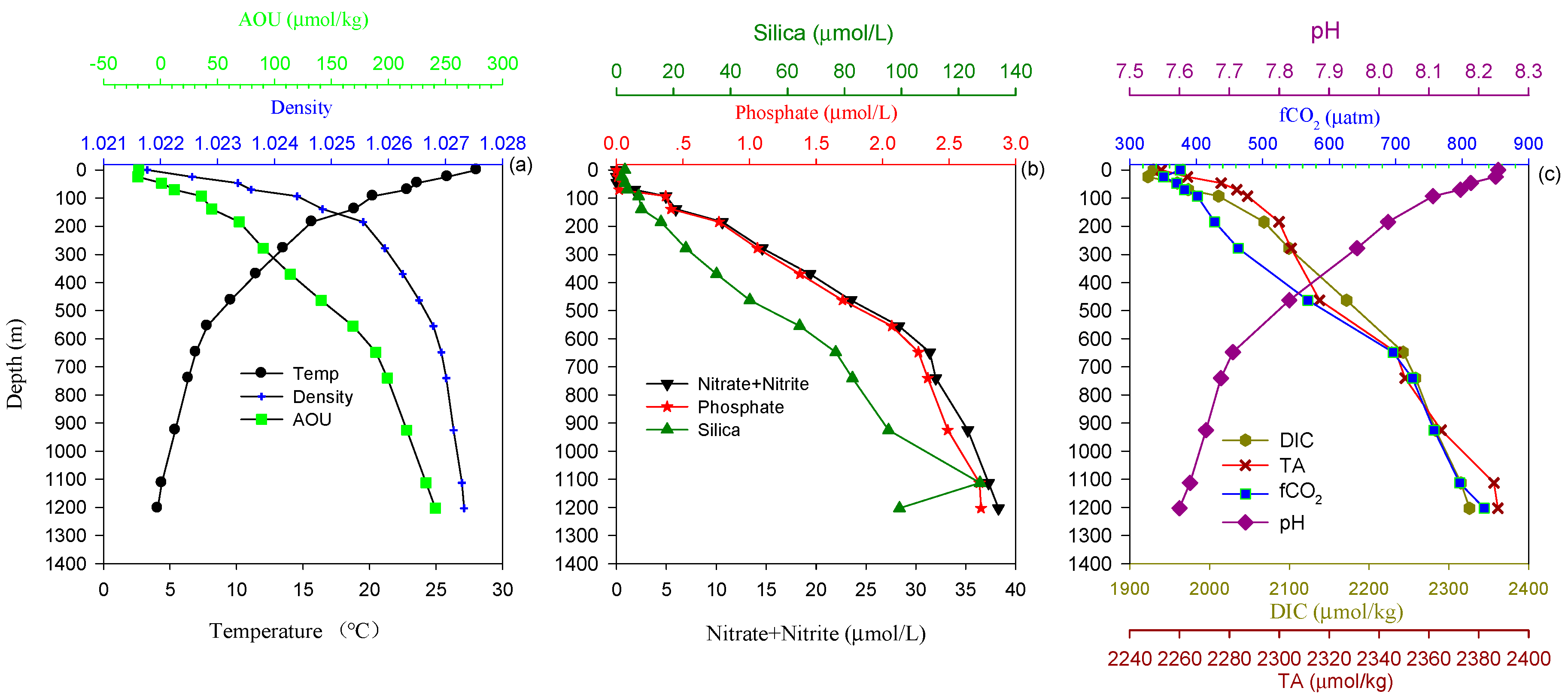
Station (Stn) T17, located at 25°00′21′′N and 122°31′54′′E, northeast of Taiwan, at a depth of 1470 m was used as a case study to show the effect of the source DOW depth and plume trapping depth on the CSEI. The typical profiles of T and S, the concentration of P, N, and Si, and the carbonate parameters of DIC, TALK, and pH at Stn T17 are depicted in Figure 3. The thermocline pattern at T17 is a typical profile with the thermocline layer from a depth of approximately 24 to approximately 200 m, with the density differences between the thermocline layer and the surface layer varying from less than 0.8 kg/m3 to 3.8 kg/m3. The raised DOW could stay at any depth in the thermocline layer after sufficient turbulent mixing when the technical settings were properly settled. According to the limited observed data at T17, depths of 24 m and 49 m were chosen to be the two sharp density interfaces to compare the effect of changing the plume trapping depth on the CSEI. The density differences between the surface and the two designated plume trapping layers are larger than 0.8 kg/m3, which is sufficient to hold the sufficiently mixed DOW plume. The apparent oxygen utilization (AOU) in water shallower than 24 m is −19 μmol/kg and changes to 1 μmol/kg at 49 m, indicating that O2 is being released by photosynthesis at depths shallower than 49 m. Thus, it is rational to deduce that, when nutrient-rich DOW was raised to 24 m or 49 m, it could stimulate active photosynthesis in those layers. According to the nutrient distribution profile, the source DOW should be deeper than approximately 90 m to reach a nutrient-rich level. According to the observed data at T17, the concentrations of phosphate, nitrate plus nitrite, and silicate in 93 m water are approximately 37, 494, and 4 times that of the 24 m water and approximately 7, 124, and 3 times that of the 46 m water, respectively. The N/P ratio of 93 m and deeper water is approximately 13.8.
In the plume trapping calculation, a two-layer system of the ocean is assumed with a homogeneous upper layer () and a plume trapping layer (). A more detailed description is available in [15,32]. Briefly, the trajectory and DOW concentration of the plume in a stratified ocean environment can be controlled by setting the flow rate, the pipe diameter, and the discharge depth in accordance with the regional current speed, the density of the source DOW, and the plume trapping depth. In such a case, an optimum plume with the highest concentration of DOW in the mixed plume ( can be formed (Figure 3). In the case of a single pipe AU system in a stratified two-layer ocean with a horizontal current speed of 0.1 m/s, a pipe radius of 0.5 m, and a pumping flow rate of 1000 m3/h at T17, 24 m and 49 m could be designated as two qualified plume trapping depths. The various parameters that form the optimized scenarios of different DOW and discharge depths are calculated according to the mathematical model described in our previous study (Table 1) [32]. When the 93 m DOW level is raised to form an optimum plume at 24 m and 49 m, respectively, at T17, the DOW should be discharged at 24 m and 52 m, respectively, based on the plume trajectory calculations. The side-view and end-view ensemble-averaged concentration fields are similar to those in Figure 2. In these two scenarios, the highest an optimum plume can reach 14.3% and 23.1%, respectively. Thus, at first, the temperature, nutrient, DIC, and TA concentration of the plume should be mixed conservatively with 85.7% ambient water and 14.3% DOW and with 76.9% ambient water and 23.1% DOW. After the phytoplankton photosynthesis following the modified Redfield ratio depletes all available nutrients as assumed, the growth of phytoplankton will cause a 16.9 μmol/kg increase in TA and a 103.1 μmol/kg decrease in the DIC of the mixed plume with a consumption of 1 μmol/kg P. The value calculated from the new TA and DIC values is depicted in Figure 4.
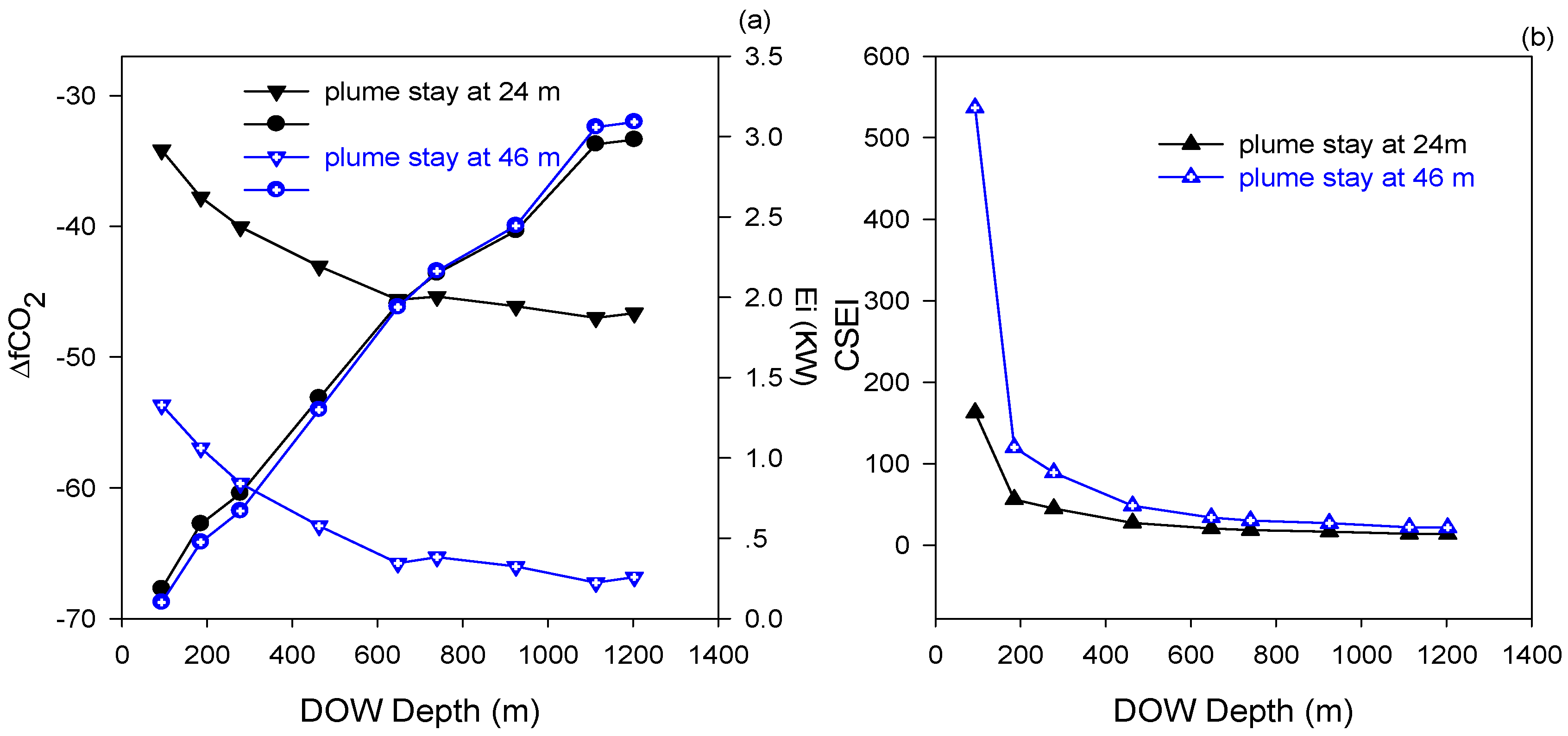
It is apparent that the CSEI is largely dependent on the source DOW depth and the plume trapping depth, as indicated in Figure 4b. In forming the optimum plume in the 24 m scenario, though the decreases from approximately −34 to −47 μatm as the source DOW depth increases from 93 to 1200 m, while the energy consumption increases from 0.21 to 3.41 KW (Figure 4a). Accordingly, the CSEI drops quickly from 163 to 56 μatm/KW as the DOW depth increases from 93 to 185 m and gradually declines to 14 μatm/KW as the DOW depth increases to 1200 m. The quickly ascending and later stabilizing pattern of CSEI versus source DOW depths indicates that the most effective method in this scenario is to raise the 93 m DOW level rather than raising the deeper DOW level. When the DOW depth is increased from 93 to 1200 m, the water becomes denser, which means that a higher mixing ratio is needed to keep it in the plume trapping layer. Although keeps decreasing when the DOW depth is increased, suggesting that a stronger carbon sequestration ability results from an increase in deeper DOW levels, the rapid energy enhancement in amplitude exceeds the variation. Considering the efficiency of unit power consumption, raising a lower DOW level to the euphotic layer is not an efficient method of sequestering atmospheric .
When the plume trapping layer moves from 24 to 46 m, the CSEI of the latter exhibits a similar pattern. The highest CSEI value reaches 537 μatm/KW when the shallowest qualified DOW level of 93 m is raised. The CSEI drops quickly to 120 μatm/KW when the source DOW level deepens to 185 m and gradually overlaps with the CSEI of the 24 m plume trapping depth after the source DOW depth increases to 463 m or more (Figure 4a). Thus, when 46 m is chosen to be the plume trapping depth, compared to the scenarios at 24 m, the range increases from −54~−67 to −34~−47 μatm, while the decreases from 0.21~3.41 to 0.10~3.09 KW, which makes the CSEI decline from 537~22 to 163~14 μatm/KW. Thus, from an energy usage point of view, keeping the plume in a qualified deeper layer will enhance carbon sequestration efficiency.
The large variations in power consumption caused by selecting different discharge depths, especially in raising higher DOW levels, are primarily due to power balance composition variations. The power needed to raise source DOW levels from different depths () is primarily composed of three parts: ,, and . and its composition when DOW depths are increased is depicted in Figure 5. The total , as well as the and , increase when the DOW depth is increased, while the remains almost constant. Although increases with considerable magnitude, it is the , the power used for covering the density difference head, that occupies more than 90% of the total power , despite the source DOW depth. In other words, the key factor in determining the total value is the density difference between the source DOW depth and the discharging depth. Comparing the total value and its composition, raising the 93 m DOW level such that it stays at depths of 24 m and 46 m, the and values quickly drop from 168 to 84 W and from 196 to 113 W, respectively, with the decline amplitude reaching approximately half of the original. When a much deeper DOW level is raised to form optimal plumes in the two depths, the decline amplitude of quickly drops from approximately 50% by raising the 93 m DOW level to 29% by raising the 185 m DOW level, and the decline amplitude slowly decline to the lowest 9% by raising the deepest DOW level (1200 m). Thus, based on a comparison between the CSEI patterns of the two plume trapping depths scenarios, the CSEI value derived from plume trapping at 46 m is not only larger than that at 24 m when the same DOW depth is raised, but the differences between them rapidly decline as the source DOW depth increases.
It must be emphasized that the simulation results are based on the basic assumptions that all of the nutrients in the DOW raised to the euphotic layer are depleted during photosynthesis. This assumption is questionable for several reasons. For instance, at Stn T17, the light intensity at the lower plume staying layer may not be sufficiently strong to support the bloom of a desirable phytoplankton species. Gong et al. (1996) reported that measured chlorophyll a (Chl a) concentrations in the southern part of the ECS in summer were roughly between 0.1 and 0.3 mg/m3 in the surface water, 1 mg/m3 in the subsurface maxima at approximately 30 m, and 0.3 mg/m3 at approximately 50 m [38]. Wang et al. (2014) reported the influence of phytoplankton growth on underwater irradiance and light fields in the ECS [39]. It could be deduced that the euphotic zone (where the downward irradiance of photosynthetic active radiation is 1% of the surface value) at which the most active photosynthetic processes occur in this region is approximately 46 m [40]. Moreover, as the relatively shallower and deeper plume trapping depths we picked in simulation are based on observed data of stations, raising the shallowest 93 m DOW level to form the highest 14.3% in the plume may cause nutrient concentration limitations in supporting the desired phytoplankton bloom. Nevertheless, the simulation results support the deduction that, in order to increase the carbon sequestration efficiency, the chosen source DOW depth should be as shallow as possible, while the chosen plume trapping depth should be as deep as possible, if the conditions in the designated trapping layer and source DOW are qualified to stimulate phytoplankton photosynthesis.
3.2. Regional Effects
To examine whether the pattern described above persists across geographies, the relationship of and CSEI with the source DOW depths was calculated using 11 other stations with latitudes from 12 to 43°N and longitudes from 110 to 137°E. Four stations in the ECS cross-shelf track [15], which are impacted by the Yangzi River, were excluded because the values at these stations were negative, regardless of the source DOW depths, indicating that, in these regions, AU will not increase the regional carbon sequestration potential. The selection of plume trapping depth and qualified DOW depth follows the same rules of Stn T17 in the ECS.
The values of most stations exhibit an apparent downward trend when the DOW depth is increased, similar to Stn T17 in the ECS. For example, the values of the formation of an optimum plume in the 10 m scenario at Stn 4 in the Sea of Japan decrease quickly from −15 μatm to −26 μatm when DOW depths increase from 52 to 307 m and then stabilize at −26 μatm after 307 m. This phenomenon should be attributed to the increasing tendency of the DOW mixing ratio of the ambient water when DOW depths are increased. Denser and deeper DOW characterized by a colder temperature and higher salinity requires higher amounts of ambient water to form optimum plumes. Thus, higher values and nutrient concentrations in DOW are generally neutralized by the ambient seawater of the discharging layer, which limits the values.
The CSEI among stations in different seas varies considerably not only among different seas but also among stations within the same sea. The highest CSEI at Stn 14 in the Sea of Japan can reach 1051 μtam/KW if 25 m DOW is raised to 10 m (Figure 6f), while, at Stns S1, S4, and S9 in the SCS, the CSEI becomes negative because the exhibits a positive value, even though the optimum technical setting has been applied, which indicates that these three stations in the SCS are not suitable for applying AU to increase the net CO2 flux (Figure 6a,b). The CSEI at Stns S40, S43, and S44 in the SCS exhibits a similar quick decline with a general stabilizing pattern. The highest CSEI value when applying AU in the SCS can reach approximately 396 μatm/KW at Stn S43 when 130 m DOW is raised and maintained at 60 m. This value quickly declines to 74 μatm/KW when the DOW level is raised to 600 m and, after that depth is reached, almost stabilizes. At Stn S40, as the sampling interval of observed data was relatively larger than those at Stns S43 and S44, the first available qualified DOW data were found at 200 m. Thus, the CSEI at S40 decreases from 267 μatm/KW at 200 m to 102 μatm/KW at 600 m and stabilizes at approximately 60 μatm/KW after 1000 m (Figure 6b). Similar decline patterns of the CSEI and changes in the CSEI slope when DOW depth is increased were also observed in the ECS and the Sea of Japan.
When comparing the CSEI with caused by AU, the opposite pattern was observed in all calculated stations in the SCS, the ECS, and the Sea of Japan, similar to Stn T17, which indicates that raising a lower DOW level to the euphotic layer can enhance the regional carbon sequestration ability but will increase power consumption. The steeper ratios of the CSEI to the DOW depth compared to the ratio of the to the DOW depth indicate a considerably sharper increase in power consumption (), compared to the value. Therefore, the CSEI values are suppressed when DOW depths are increased. In addition, the CSEI range in the scenario of a deeper plume usually exceeds that of a shallower plume. The gaps between the CSEI values are compressed when the DOW depth is increased up to a certain point. The phenomena indicate that deepening the plume trapping level can increase carbon sequestration efficiency; however, the amplitude decreases when the DOW depth is increased. The regional effects on and the CSEI pattern suggest that it is not worth raising extremely deep DOW levels to the upper layer in a settled AU applied region. Furthermore, the regional CSEI and can vary within a large range when AU is applied in different regions.
3.3. Seasonal Effects
Seasonal effects on the CSEI of AU were analyzed using data from S43 and ST6, S44 and ST17 (SCS), T17 and Stn 12 (ECS), as well as Stn14 and KS3634 (Sea of Japan). These stations are adjacent, but the data were acquired in summer and winter, respectively.
Due to the strength of winter monsoons and the cooling of surface temperature, the water column in the SCS and ECS was well-mixed, with the mixed-layer depth (MLD) deepening from summer to winter [40,41,42]. Liu et al. (2002) observed a deeper subsurface Chl a maximum (SCM) at 75 m in September 1998 and a shallower SCM at 40 ~ 50 m at the same site in January 1999 in the Northern SCS [43]. Comparing the thermocline profiles between Stn T17 in summer and Stn 12 in winter, the MLD deepens from 24 to ~52 m with the AOU values of approximately −7.4 and 0, respectively. If the plume trapping depth is lowered to a depth of 76 m, the light intensity at that depth will not be sufficiently strong to support a bloom of phytoplankton. If we move the plume trapping depth from 52.4 to 30.5 m, which is close to the optimal plume trapping depth (24 m) in summer, the DOW cannot be trapped at the well-mixed layer. Thus, a 30.5 m depth cannot serve as a plume trapping layer because the density distribution of the mixed-layer is greater—even in winter—and the density difference between DOW and the top thermocline layer is smaller in winter than it is in summer. The plume trapping depths were chosen at the top of the thermocline layer—49 m at Stn 12 in the ECS. Regardless, due to the density profile in winter, only a DOW level that is shallower than 400 m can be sufficiently mixed to stay in the euphotic layer at Stn 12. Similar situations were also observed in the SCS. Thus, at the same site (Stn S43 in summer and ST17 in winter; Stn S44 in summer and ST6 in winter), the plume staying depths were chosen at 60 m—the top of the thermocline layer. In the winter, the regional sea near Stn 14 and KS3634 in the Sea of Japan is characterized by strong stratification with a thin layer of low salinity and high temperature water overlay the top 60 m of the water column [26,44]. The top overlay water shows near equal density (~1025.6 kg/m³) from the surface to 27 m. The existence of well-mixed mixed-layer water and strong pycnocline in winter makes it impossible to raise the DOW level such that it remains in the mixed layer, which is between the surface and a 27 m depth. The positive AOU and nitrate value at 51 m suggest that a depth of 51 m was not a proper environment to stimulate primary production. Thus, due to a lack of sampling data with respect to DOW levels from 27 to 51 m, we added a layer between 27 and 51 m, assuming the physical and chemical parameters to be the average between these layers. Due to these factors, when comparing the effect of seasonal differences, comparisons between different plume trapping depth scenarios were not made. The plume staying depth was chosen at 39 m at Stn KS3634 (in the Sea of Japan) in winter.
Comparing both the and CSEI values between summer and winter, differences in the AU effect on the regional carbon sequestration efficiency in summer and winter were observed, although the CSEI vs. DOW depth patterns are similar (Figure 7). In the SCS, the range in the region of ST17 (in winter) and S43 (in summer) increases from −9~−130 to −80~−117 μatm, and the CSEI decreases from 550~70 to 400~70 μatm/KW, which indicates that a stronger carbon sequestration effect and a higher sequestration efficiency can be achieved in winter. However, in the region of ST6 (in winter) and S44 (in summer), the opposite phenomenon was observed. Both the and the CSEI indicate that a higher carbon sequestration effect can be achieved in summer when applying AU in that region (Figure 7a,b). In the ECS, the range of the regional sea around Stn 12 changes from −54~−67 μatm in summer to −15~−16 μatm in winter, and the CSEI decreases from the range of 537~22 μatm/KW in summer to 59~14 μatm/KW in winter, suggesting that a higher carbon sequestration effect could be achieved in summer in the ECS. In the Sea of Japan, both and the CSEI in winter shows a greater carbon sequestration ability than that in summer. Although the CSEI in winter reaches ~1000 μatm/KW when raising the shallowest 25 m DOW to 10 m in summer, a considerably higher CSEI value of ~6000 μatm/KW could be observed when raising 50 m DOW to 39 m in winter. Thus, although high carbon sequestration efficiency can be achieved in the Sea of Japan in both summer and winter seasons, winter is a better season to apply the AU.
Based on the differences between summer and winter in the simulated regional effects of AU, no definitive conclusion as to which season is best for applying AU can be made. Specific problems should be evaluated on a case-by-case basis.
4. Discussion
It was demonstrated in our previous paper that the contribution of AU in the conversion of a region from a strong source to sink was dependent on the applied region, the season, and the technical parameters of the AU [15]. In this study, we calculated the energy consumption between different source DOW depths and discharge depths using 16 stations. The simulation results indicate that the optimum DOW depth varies with different regions and seasons. However, the optimum DOW depth usually appears at depths of approximately 100~200 m, except for application of AU at Stn 14 in the Sea of Japan. In most of the applied regions, the CSEI values from raising a DOW level deeper than 300 m usually maintain a slowly declining or stabilizing pattern, which indicate that, as an atmospheric sequestration tool, it is not necessary to incur the extremely high cost of raising deeper DOW levels. On the contrary, raising qualified shallower DOW levels can achieve high sequestration efficiency.
The assumptions, including the carbon-to-nutrient ratio, the complexity of the marine ecological system, whether nutrients can be depleted during photosynthesis, and whether all of the inorganic carbon transferred to organic carbon can be transported to below the mixed layer, should all be taken into consideration. Although these assumptions have been discussed in [15] and are commonly made in carbonate transformation calculations, the uncertainties behind the assumptions are worth emphasizing. When the DOW was raised to a designated depth, the plume composition was determined by the technical settings of AU, which would change the physical and chemical parameters in the plume, including the nutrients and the inorganic carbonate parameters, and thus the value of the plume. The first hypothesis, that an optimum plume in a designated sub-layer can be formed if the technical settings are adjusted in accordance with regional conditions, is valid, which has been proved by numerical simulation [32], lab experiments, and sea trial monitoring. The second hypothesis, that phytoplankton photosynthesis is assumed to deplete all available nutrients in the raised DOW following the modified Redfield ratio C/H/O/N/S/P = 103.1/181/93/11.7/2.1/1 [33,34], where P is assumed to be the limiting nutrient, is questionable. Firstly, whether the nutrients can be depleted or not is greatly influenced by the physical and chemical condition in the DOW plume—for instance, whether the light intensity and the temperature is suitable for supporting the phytoplankton bloom or whether the nutrient and the inorganic carbonate concentration in the plume could stimulate the desired phytoplankton bloom. Secondly, whether the phytoplankton photosynthesis follows the modified Redfield ratio is important in terms of the accuracy of the simulated uptake efficiency; however, the stoichiometric relationship is questionable. The Redfield C/N/P ratio for phytoplankton is not a universally optimal value. It represents an average for a diverse oceanic phytoplankton assemblage growing under a variety of different conditions and employing a range of growth strategies. Thus, the C/N/P ratio used in calculating the carbon fixation of a particular region is controlled by both oceanic phytoplankton species and their growth strategies acclimated to the environment. Therefore, the C/N/P ratio would be greatly influenced by the physical and chemical condition in the plume. The modified Redfield ratio of particulate organic matter from the SCS, the ECS, the Taiwan Strait, the Sea of Japan, and the related outer estuaries (S > 25) and river plumes used in the simulation reflect the average effects of oceanic phytoplankton assemblage, which make the assumption rational in the carbon sequestration calculation. Thirdly, the assumption that P is the limiting nutrient is also questionable but might be rational, since the existence of nitrogen fixation is caused by the exclusively prokaryotic metabolic process [35]. Moreover, that the extreme complexity of the AU-induced carbon sequestration process makes the feasibility and benefits of AU stimulate ocean productivity remains controversial [45,46,47]. Although a consistent increase in phytoplankton biomass and a primary production increase were reported by all five ship-based experiments, with a demonstrated shift in phytoplankton communities from small (<2 µm diameter) to large (>10 µm diameter) diatom cells, the biogeochemical consequences of sustained upwelling are uncertain and the overall effectiveness of enhanced marine photosynthesis is uncertain especially with regard to the long term [48,49]. Another point that needs to be emphasized, especially before the large-scale application of AU, is the undesirable and uncertain impacts caused by AU, including aggravation of acidification [9,50], the surface temperature, and salinity change [51], and the disturbance of upper and seafloor ocean ecosystems [22,23,52]. Kwiatkowski et al. reported that, if enhanced upwelling is carried out on a sufficiently large scale and for a sufficiently long period of time, the ocean thermocline might be disrupted, which may cause long-term warming of the climate system [51]. Nevertheless, it is still desirable for national or international investment in AU as potential technical reserves. The complexity of the impact of AU in the marine system and climate system should not be an obstacle to its investigation. However, cautions must be observed when applying AU in the sea trial, even if its deployment is not large-scale. Still, the simulation results of this study help to evaluate the potential uptake effect and efficiency. The results also point out the close relationship among the atmospheric uptake efficiency, the technical settings of the AU, and the applied region and season.
Considering the power consumption calculation, as the DOW density changes with different depths of source DOW, the optimum discharge depth should be modulated to make the DOW plume stay at the designated plume trapping depth. Since the energy consumption calculation of is a complex function of pipe length and the density of a pipe’s lower end and upper end seawater (Equation (11)), the optimum depths in calculation are roughly simplified to be the depth of the density interface. Taking Stn T17 profile data as an example, the modified of creating an optimum plume at 24 m and 46 m varies from 24 to 21.8 m and from 45.3 to 43.1 m, respectively, when the source DOW level deepens from 93 to 1203 m. The maximum variation of calculated and CSEI are thus within the range of 1%, which indicates that it is rational to use the instead of the for simplification. Additionally, in considering power consumption, although the power balance equation for air-lift pump AU based on [16] was extended to include the effects of the gas void fraction and the local head loss in [36], it did not include the effects of the local head loss produced by devices and blockages, such as nozzles, valves, pipe bends, enlargements, contractions, or the adhesion of marine fouling organisms in the upwelling pipe. Nevertheless, simulation results are meaningful especially for the large-scale application of AU. White et al. (2010) reported that a custom prototype wave pump failed after 17 h of delivery from a 300 m DOW level to the surface [19]. The failure might be partly attributed to improper deployment strategies [53,54]. Ouchi et al. (2005) reported a raised high-density 220 m DOW sinking to the euphotic layer in an open ocean AU experiment [18]. A new prototype with a density current generator was thus developed to minimize the sinking problem [20]. According to the simulation results, the applied upwelling region would exhibit a strong carbon source status and achieve its highest carbon sequestration efficiency with shallower DOW raised when proper engineering design is achieved in technical parameters, which include source DOW depth, pipe diameter, flux flow rate, and discharging depth. It is possible that, in AU sea trials, raising a considerably shallower DOW could have met the demand and achieved a higher CSEI value and thereby greatly reduced the risk of failure.
Comparing the range of and CSEI values among applications in different regions, CSEI varies over a considerably wider range. This phenomenon should probably be attributed to the regional density profile differences. When applying an AU to sequester atmospheric , the effects of the different types of density profiles on the CSEI should be taken into consideration. Thus, when applying AU as a geoengineering tool to sequester atmospheric , in order to achieve higher sequestration efficiency and reduce the risks and expenses in deploying the device, the regional and seasonal carbonate and nutrient vertical distributions should be considered, as should the density profile, which is a non-negligible parameter. Further investigative research should be performed to compare the CSEI of AU in regions with different density profiles.
Although we focused here on the relationship among uptake effect and efficiency, power demand, technical settings, and the related applied region and season, the power supply strategy is of major importance for the AU’s working duration and mission completion. A self-powered technology is crucial for applying AU far away from the shore. The renewable energy should be preferable to AU to assure feasibility and sustainability. Research on renewable energy for the task of raising DOW levels has focused on using offshore wind for mariculture applications [55], using wave energy for phytoplankton bloom stimulation [19], and using perpetual salt fountain to increase primary production [56,57]. A distributed generation (DG) power supply system that consists of DG units of a wind turbine, a wave energy converter (WEC) array, a PV array, and a diesel generator was investigated by our group and utilized in air-lift AU [17]. As a potential carbon sequestration technology, the ratio of potential emissions caused by the power supply to potential (short-term and long-term) uptake due to AU is crucial and should be given consideration in future research.
5. Conclusions
In this study, we simulated the power () needed to raise the source DOW to designated plume trapping depths using observed carbon and nutrient data from 16 stations in the SCS, the ECS, and the Sea of Japan, with latitudes ranging from 12°N to 43°N. The power needed to raise the source DOW from different depths could be primarily divided into three parts, from which the power demand of the density difference head consumes more than 90% of the total power, regardless of the source DOW depth. Thus, from an efficiency point of view, the key factors that determine the total power are the density differences between the source DOW depth and the plume trapping depth.
The CSEI was defined by dividing the by to indicate the uptake ability per unit of power consumption. The results suggest that, in most of the applied regions, as the enhancement amplitude of value exceeds the value when the DOW depth is increased, CSEI and exhibit an opposite pattern. Large variations in the CSEI were shown to be associated with different regional, seasonal, and AU technical parameters. Thus, from an energy efficiency point of view, AU should be designed to raise the shallowest qualified DOW to the deepest qualified plume trapping depth to achieve the highest CSEI. According to the simulation results, raising extremely deep DOW to discharging depth not only is energy-inefficient but also brings several related challenges that exist in designing and fabricating a technologically robust device with longer pipes. AU may have potential as a geoengineering technique that achieves high energy efficiency in anthropogenic uptake, if enacted in the right regions under optimal seasonal conditions and technical parameters. According to simulation results, the largest CSEI is at Stn 14 in the Sea of Japan when a 25 m DOW level was raised to 10 m, suggesting that the northeast past of the Sea of Japan is most suitable for AU. The CSEI at Stn S1, S4, and S9 in the SCS becomes negative, despite an optimum technical setting, indicating that applying AU to increase the net flux in some regions of the SCS is inappropriate.
Acknowledgments
This research work was funded by the National Natural Science Funds of China (Grant No. 41776084 and 41406084), the International Science & Technology Cooperation Program of China (Grant no. 2015DFA01410), and Taiwan’s Aim for the Top University Program (04C030204). We thank the reviewers for their constructive comments.
Author Contributions
Yiwen Pan and Wei Fan conceived and designed the simulation method and wrote the draft. Long You and Yifan Li analyzed and processed the data. Chen-Tung Arthur Chen and Ying Chen provided data and added valuable comments during the draft writing. Bing-Jye Wang contributed partial data collection and prepared figures.
Conflicts of Interest
The authors declare no conflict of interest.
References
- Lovelock, J.E.; Rapley, C.G. Ocean pipes could help the Earth to cure itself. Nature 2007, 449, 403. [Google Scholar] [CrossRef] [PubMed]
- Williamson, P.; Turley, C. Ocean acidification in a geoengineering context. Philos. Trans. A Math. Phys. Eng. Sci. 2012, 370, 4317–4342. [Google Scholar] [CrossRef] [PubMed]
- Handå, A.; McClimans, T.A.; Reitan, K.I.; Knutsen, Ø.; Tangen, K.; Olsen, Y. Artificial upwelling to stimulate growth of non-toxic algae in a habitat for mussel farming. Aquac. Res. 2013, 45, 1798–1809. [Google Scholar] [CrossRef]
- Ianson, D.; Allen, S.E. A two-dimensional nitrogen and carbon flux model in a coastal upwelling region. Glob. Biogeochem. Cycles 2002, 16. [Google Scholar] [CrossRef]
- Chung, C.-C.; Gong, G.-C.; Hung, C.-C. Effect of Typhoon Morakot on microphytoplankton population dynamics in the subtropical Northwest Pacific. Mar. Ecol. Prog. Ser. 2012, 448, 39–49. [Google Scholar] [CrossRef]
- Jiang, Z.-P.; Huang, J.-C.; Dai, M.; Ji Kao, S.; Hydes, D.J.; Chou, W.-C.; Jan, S. Short-term dynamics of oxygen and carbon in productive nearshore shallow seawater systems off Taiwan: Observations and modeling. Limnol. Oceanogr. 2011, 56, 1832–1849. [Google Scholar] [CrossRef]
- Oschlies, A.; Pahlow, M.; Yool, A.; Matear, R. Climate engineering by artificial ocean upwelling: Channelling the sorcerer’s apprentice. Geophys. Res. Lett. 2010, 37, 1–5. [Google Scholar] [CrossRef]
- Yool, A.; Shepherd, J.G.; Bryden, H.L.; Oschlies, A. Low efficiency of nutrient translocation for enhancing oceanic uptake of carbon dioxide. J. Geophys. Res. 2009, 114. [Google Scholar] [CrossRef] [Green Version]
- Keller, D.P.; Feng, E.Y.; Oschlies, A. Potential climate engineering effectiveness and side effects during a high carbon dioxide-emission scenario. Nat. Commun. 2014, 5, 3304–3315. [Google Scholar] [CrossRef] [PubMed] [Green Version]
- Le Quere, C.; Andrew, R.M.; Canadell, J.G.; Sitch, S.; Korsbakken, J.I.; Peters, G.P.; Manning, A.C.; Boden, T.A.; Tans, T.T.; Houghton, T.A.; et al. Global carbon budget 2016. Earth Syst. Sci. Data 2016, 8, 605–649. [Google Scholar] [CrossRef]
- Liu, K.-K.; Atkinson, L.; Chen, C.T.A.; Gao, S.; Hall, J.; MacDonald, R.W.; McManus, L.T.; Quiñones, R. Exploring continental margin carbon fluxes on a global scale. Eos Trans. Am. Geophys. Union 2000, 81, 641–644. [Google Scholar] [CrossRef]
- Painting, S.J.; Lucas, M.I.; Peterson, W.T.; Brown, P.C.; Hutchings, L.; Mitchell-Innes, B.A. Dynamics of bacterioplankton, phytoplankton and mesozooplankton communities during the development of an upwelling plume in the southern Benguela. Mar. Ecol. Ser. 1993, 100, 35–53. [Google Scholar] [CrossRef]
- Cai, W.-J.; Dai, M.; Wang, Y. Air-sea exchange of carbon dioxide in ocean margins: A province-based synthesis. Geophys. Res. Lett. 2006, 33, 347–366. [Google Scholar] [CrossRef]
- Sobarzo, M.; Bravo, L.; Donoso, D.; Garcés-Vargas, J.; Schneider, W. Coastal upwelling and seasonal cycles that influence the water column over the continental shelf off central Chile. Prog. Oceanogr. 2007, 75, 363–382. [Google Scholar] [CrossRef]
- Pan, Y.; Fan, W.; Huang, T.-H.; Wang, S.-L.; Chen, C.A. Evaluation of the sinks and sources of atmospheric CO2 by artificial upwelling. Sci. Total Environ. 2015, 511, 692–702. [Google Scholar] [CrossRef] [PubMed]
- Liang, N.; Peng, H. A study of air-lift artificial upwelling. Ocean Eng. 2005, 32, 731–745. [Google Scholar] [CrossRef]
- Zhang, D.; Fan, W.; Yang, J.; Pan, Y.; Chen, Y.; Huang, H.; Chen, J. Reviews of power supply and environmental energy conversions for artificial upwelling. Renew. Sustain. Energy Rev. 2016, 56, 659–668. [Google Scholar] [CrossRef]
- Ouchi, K.; Otsuka, K.; Omura, H. Recent Advances of Ocean Nutrient Enhancer “TAKUMI” Project. In Proceedings of the Sixth ISOPE Ocean Mining Symposium, Changsha, China, 9–13 October 2005; pp. 7–12. [Google Scholar]
- White, A.; Björkman, K.; Grabowski, E.; Letelier, R.; Poulos, S.; Watkins, B.; Karl, D. An Open Ocean Trial of Controlled Upwelling Using Wave Pump Technology. J. Atmos. Ocean. Technol. 2010, 27, 385–396. [Google Scholar] [CrossRef]
- Tsubaki, K.; Maruyama, S.; Komiya, A.; Mitsugashira, H. Continuous measurement of an artificial upwelling of deep sea water induced by the perpetual salt fountain. Deep Sea Res. Part I Oceanogr. Res. Pap. 2007, 54, 75–84. [Google Scholar] [CrossRef]
- Maruyama, S.; Tsubaki, K.; Taira, K.; Sakai, S. Artificial Upwelling of Deep Seawater Using the Perpetual Salt Fountain for Cultivation of Ocean Desert. J. Oceanogr. 2004, 60, 563–568. [Google Scholar] [CrossRef]
- Aure, J.; Strand, Ø.; Erga, S.; Strohmeier, T. Primary production enhancement by artificial upwelling in a western Norwegian fjord. Mar. Ecol. Prog. Ser. 2007, 352, 39–52. [Google Scholar] [CrossRef]
- McClimans, T.A.; Handå, A.; Fredheim, A.; Lien, E.; Reitan, K.I. Controlled artificial upwelling in a fjord to stimulate non-toxic algae. Aquac. Eng. 2010, 42, 140–147. [Google Scholar] [CrossRef]
- Pan, Y.W.; Fan, W.; Zhang, D.H.; Chen, J.W.; Huang, H.C.; Liu, S.X.; Jiang, Z.P.; Di, Y.N.; Tong, M.M.; Chen, Y. Research progress in artificial upwelling and its potential environmental effects. Sci. China Earth Sci. 2016, 59, 236–248. [Google Scholar] [CrossRef]
- Japan Meteorological Agency. Data of oceanographic and marine meteorological observation. Available online: http://www.data.jma.go.jp/gmd/kaiyou/db/vessel_obs/data-report/html/ship/ship_e.php (accessed on 25 February 2018).
- Chen, C.-T.A.; Wang, S.-L.; Bychkov, A.S. Carbonate chemistry of the Sea of Japan. J. Geophys. Res. 1995, 100, 13737–13745. [Google Scholar] [CrossRef]
- Chen, C.-T.A.; Wang, S.-L. Carbon, alkalinity and nutrient budgets on the East China Sea continental shelf. J. Geophys. Res. 1999, 104, 20675–20686. [Google Scholar] [CrossRef]
- Chen, C.A.; Wang, S.-L. International intercalibration of carbonate parameters. Acta Oceanol. Sin. 1993, 15, 60–67. [Google Scholar]
- Lewis, E.; Wallace, D. Program Developed for CO2 System Calculations; Oak Ridge National Laboratory: Oak Ridge, TN, USA, 1998.
- Mehrbach, C.C.H.; Culberson, J.H.; Hawley Pytkowicz, R.M. Measurements of the apparent dissociation constants of carbonic acid in seawater at atmospheric pressure. Limnol. Oceanogr. 1973, 18, 897–907. [Google Scholar] [CrossRef]
- Weiss, R.F. Carbon dioxide in water and seawater: The solubility of a non-ideal gas. Mar. Chem. 1974, 2, 203–215. [Google Scholar] [CrossRef]
- Fan, W.; Pan, Y.; Liu, C.C.K.; Wiltshire, J.C.; Chen, C.-T.A.; Chen, Y. Hydrodynamic design of deep ocean water discharge for the creation of a nutrient-rich plume in the South China Sea. Ocean Eng. 2015, 108, 356–368. [Google Scholar] [CrossRef]
- Chen, C.A.; Gong, G.-C.; Wang, S.-L.; Bychkov, A.S. Redfield ratios and regeneration rates of particulate matter in the Sea of Japan as a model of closed system. Geophys. Res. Lett. 1996, 24, 1785–1788. [Google Scholar] [CrossRef]
- Chen, C.-T.A.; Lin, C.-M.; Huang, B.-T.; Chang, L.-F. Stoichiometry of carbon, hydrogen, nitrogen, sulfur and oxygen in the particulate matter of the western North Pacific marginal seas. Mar. Chem. 1996, 54, 179–190. [Google Scholar] [CrossRef]
- Karl, D.; Letelier, R.; Tupas, L.; Dore, J.; Christian, J.; Hebel, D. The role of nitrogen fixation in biogeochemical cycling in the subtropical North Pacific Ocean. Nature 1997, 388, 533–538. [Google Scholar] [CrossRef]
- Fan, W.; Chen, J.; Pan, Y.; Huang, H.; Arthur Chen, C.-T.; Chen, Y. Experimental study on the performance of an air-lift pump for artificial upwelling. Ocean Eng. 2013, 59, 47–57. [Google Scholar] [CrossRef]
- Gu, Y.Z. Friction factor of fluids in pipes. Chem. Eng. 1936, 3, 3–14. [Google Scholar]
- Gong, G.-C.; Lee Chen, Y.-L.; Liu, K.-K. Chemical hydrography and chlorophyll a distribution in the East China Sea in summer: implications in nutrient dynamics. Cont. Shelf Res. 1996, 16, 1561–1590. [Google Scholar] [CrossRef]
- Wang, S.Q.; Ishizaka, J.; Yamaguchi, H.; Tripathy, S.C.; Hayashi, M.; Xu, Y.J.; Mino, Y.; Matsuno, T.; Watanabe, Y.; Yoo, S.J. Influence of the Changjiang River on the light absorption properties of phytoplankton from the East China Sea. Biogeosciences 2014, 11, 1759–1773. [Google Scholar] [CrossRef]
- Koshikawa, H.; Higashi, H.; Hasegawa, T.; Nishiuchi, K.; Sasaki, H.; Kawachi, M.; Kiyomoto, Y.; Takayanagi, K.; Kohata, K.; Murakami, S. Assessing depth-integrated phytoplankton biomass in the East China Sea using a unique empirical protocol to estimate euphotic depth. Estuar. Coast. Shelf Sci. 2015, 153, 74–85. [Google Scholar] [CrossRef]
- Zhang, W.; Wang, H.; Chai, F.; Qiu, G. Physical drivers of chlorophyll variability in the open South China Sea. J. Geophys. Res. Oceans 2016, 121, 7123–7140. [Google Scholar] [CrossRef]
- Hung, C.-C.; Gong, G.-C. Biogeochemical Responses in the Southern East China Sea After Typhoons. Oceanography 2011, 24, 42–51. [Google Scholar] [CrossRef]
- Liu, K.-K.; Chao, S.-Y.; Shaw, P.-T.; Gong, G.-C.; Chen, C.-C.; Tang, T.Y. Monsoon-forced chlorophyll distribution and primary production in the South China Sea: Observations and a numerical study. Deep Sea Res. Part I Oceanogr. Res. Pap. 2002, 49, 1387–1412. [Google Scholar] [CrossRef]
- You, Y.; Chang, K.I.; Yun, J.Y.; Kim, K.R. Thermocline circulation and ventilation of the East/Japan Sea, part I: Water-mass characteristics and transports. Deep Sea Res. Part II Top. Stud. Oceanogr. 2010, 57, 1221–1246. [Google Scholar] [CrossRef]
- Boyd, P.W. Ocean Fertilization for Sequestration of Carbon Dioxide from the Atmosphere. In Geoengineering Responses to Climate Change; Lenton, T., Vaughan, N., Eds.; Springer: New York, NY, USA, 2013; pp. 53–72. [Google Scholar]
- Council, N.R. Climate Intervention: Carbon Dioxide Removal and Reliable Sequestration; The National Academies Press: Washington, DC, USA, 2015; p. 140. [Google Scholar]
- Williamson, P.; Wallace, D.W.R.; Law, C.S.; Boyd, P.W.; Collos, Y.; Croot, P.; Denman, K.; Riebesell, U.; Takeda, S.; Vivian, C. Ocean fertilization for geoengineering: A review of effectiveness, environmental impacts and emerging governance. Process Saf. Environ. Protect. 2012, 90, 475–488. [Google Scholar] [CrossRef]
- Secretariat of the Convention on Biological Diversity. Scientific Synthesis of the Impacts of Ocean Fertilization on Marine Biodiversity; CBD Technical Series: Quebec, QC, Canada, 2009; pp. 45–53. [Google Scholar]
- Williamson, P.; Bodle, R. Update on Climate Geoengineering in Relation to the Convention on Biological Diversity: Potential Impacts and Regulatory Framework; CBD Technical Series: Quebec, QC, Canada, 2016; pp. 84–158. [Google Scholar]
- Bauman, S.; Costa, M.; Fong, M.; House, B.; Perez, E.; Tan, M.; Thornton, A.; Franks, P. Augmenting the Biological Pump: The Shortcomings of Geoengineered Upwelling. Oceanography 2014, 27, 17–23. [Google Scholar] [CrossRef]
- Kwiatkowski, L.; Ricke, K.L.; Caldeira, K. Atmospheric consequences of disruption of the ocean thermocline. Environ. Res. Lett. 2015, 10, 1–9. [Google Scholar] [CrossRef]
- Aspetsberger, F.; Zabel, M.; Ferdelman, T.; Struck, U.; Mackensen, A.; Ahke, A.; Witte, U. Instantaneous benthic response to different organic matter quality: In situ experiments in the Benguela Upwelling System. Mar. Biol. Res. 2007, 3, 342–356. [Google Scholar] [CrossRef]
- Kithil, P.W. Comments on “An Open Ocean Trial of Controlled Upwelling Using Wave Pump Technology”. J. Atmos. Ocean. Technol. 2011, 28, 847–849. [Google Scholar] [CrossRef]
- White, A.E.; Letelier, R.M.; Björkman, K.M.; Grabowski, E.; Poulos, S.; Watkins, B.V.; Karl, D.M. Reply. J. Atmos. Ocean. Technol. 2010, 28, 850–851. [Google Scholar] [CrossRef]
- Viúdez, Á.; Balsells, M.F.-P.; Rodríguez-Marroyo, R. Artificial upwelling using offshore wind energy for mariculture applications. Sci. Mar. 2016, 80, 235–248. [Google Scholar] [CrossRef]
- Stommel, H.; Arons, A.B.; Blanchard, D. An oceanographical curiosity: the perpetual salt fountain. Deep Sea Res. 1956, 3, 152–153. [Google Scholar] [CrossRef]
- Maruyama, S.; Yabuki, T.; Sato, T.; Tsubaki, K.; Komiya, A.; Watanabe, M.; Kawamura, H.; Tsukamoto, K. Evidences of increasing primary production in the ocean by Stommel’s perpetual salt fountain. Deep Sea Res. Part I Ocean. Res. Pap. 2011, 58, 567–574. [Google Scholar] [CrossRef]
Figure 1.
Map of the study area. Red triangles indicate the stations that were sampled in summer from cruises of KEEP-MASS and OR-I 728; yellow circles indicate the locations where samples were collected in winter from cruises OR-I 508, OR-I 237 and the Keifu Maru.
Figure 1.
Map of the study area. Red triangles indicate the stations that were sampled in summer from cruises of KEEP-MASS and OR-I 728; yellow circles indicate the locations where samples were collected in winter from cruises OR-I 508, OR-I 237 and the Keifu Maru.
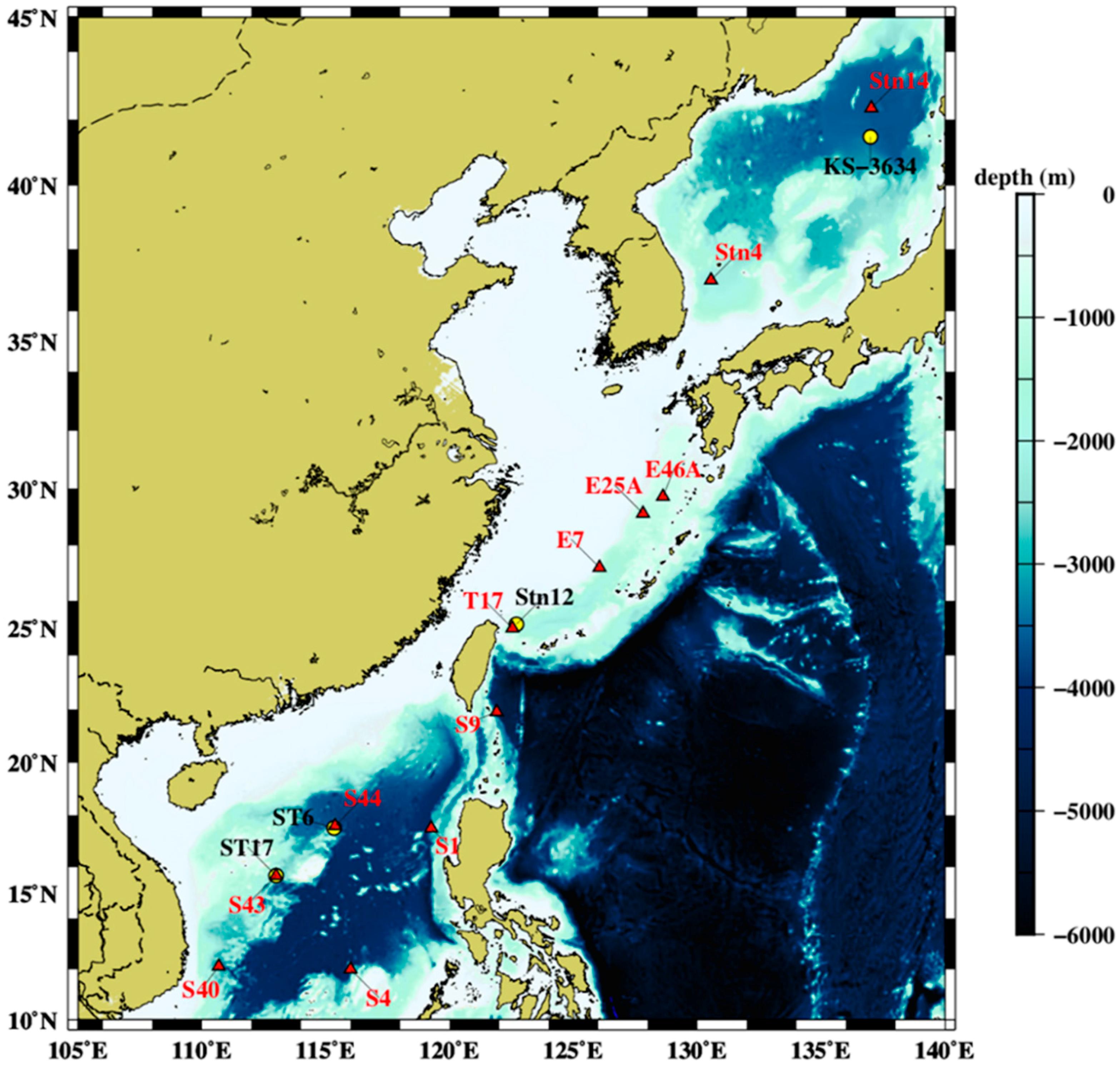
Figure 2.
Side-view (a) and end-view (b) ensemble-averaged concentration fields at 30 m from the nozzle for the optimized scenarios [15]. When the current speed is 0.1 m/s, the radius of the upwelling pipe is 0.5 m, and the water volumetric flow rate is 1000 m3/h, in order to raise the DOW by ~200 m to form an optimum plume at 21 m, the discharge depth should be set to approximately 4.5 m above the density interface at 22°09′86′′N and 118°23′47′′E in the SCS.
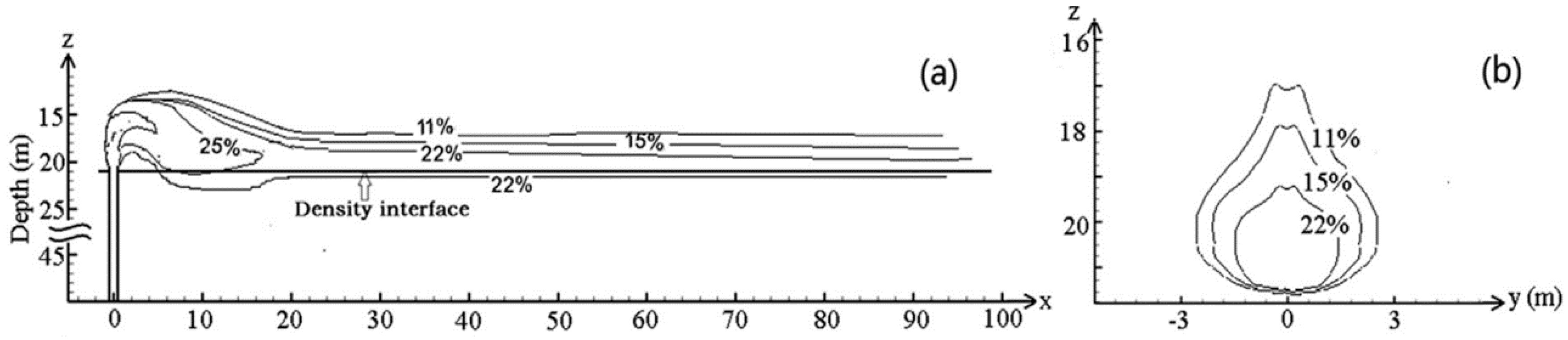
Figure 3.
Typical temperature, density, AOU, nutrients, and carbonate profiles in Stn T17. (a) temperature, density and AOU profiles [15] (b) nutrients profiles [15] (c) carbonate profiles.

Figure 4.
The effects of changing the source DOW depth and plume trapping depth on carbon sequestration ability, power consumption, and carbon sequestration efficiency at Stn T17 in the ECS. (a) and versus source DOW depth; the black solid downward triangles and circles represent and when the plume stays at 24 m, whereas the blue hollow downward triangles and circles represent and when the plume stays at 46 m. (b) CSEI versus source DOW depth; the black solid and the blue hollow symbols indicate the CSEI when a plume is formed at 24 m and 46 m, respectively.

Figure 5.
Power consumption and its composition with different source DOW depths. The bar on the left is the composition when discharging at a shallower depth to form a plume at 24 m and the bar on the right represents the composition when discharging at a deeper depth to form a plume at 46 m.
Figure 5.
Power consumption and its composition with different source DOW depths. The bar on the left is the composition when discharging at a shallower depth to form a plume at 24 m and the bar on the right represents the composition when discharging at a deeper depth to form a plume at 46 m.
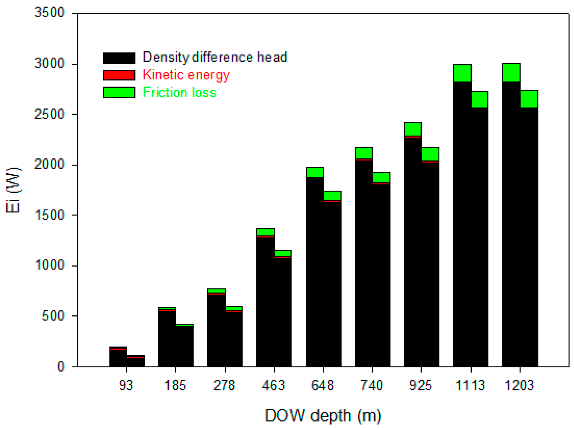
Figure 6.
Regional effects on and CSEI values with increasing source DOW depths in (a,b) the SCS, (c,d) the alongshore track in the ECS, (e,f) the Sea of Japan. Solid symbols indicate the and CSEI values of a plume formed at a shallower depth, and the hollow ones indicate the CSEI of a plume at a deeper depth.
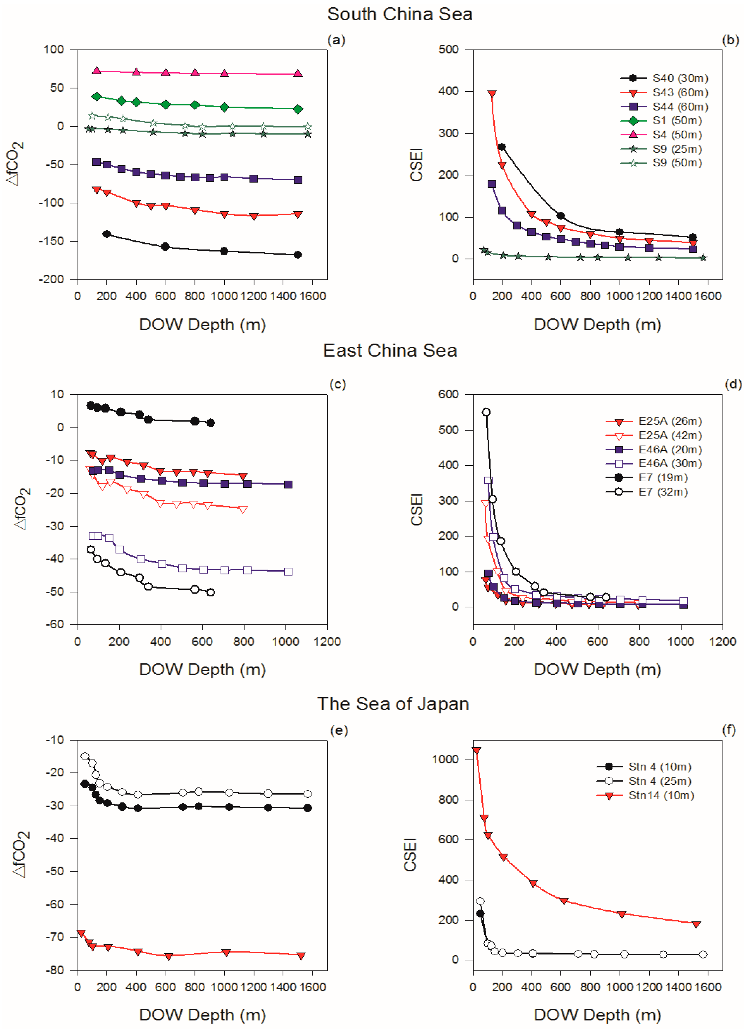
Figure 7.
Seasonal effects on and CSEI values versus increasing source DOW depths in (a,b) the SCS, (c,d) in the ECS, (e,f) in the Sea of Japan. The hollow symbols with dashed lines indicate the and CSEI values are calculated based on the assumption that the plume would stay in a manually added intermediate layer 39 m, with all of the physical and chemical data on average between the sampling depths of 27 and 51 m.


Table 1.
Technical parameters for creating an optimum plume at 24 m and 46 m, respectively, at Stn T17 in the ECS, assuming a horizontal current speed of 0.1 m/s, a pipe radius of 0.5 m, and a pumping flow rate of 1000 m3/h.
Table 1.
Technical parameters for creating an optimum plume at 24 m and 46 m, respectively, at Stn T17 in the ECS, assuming a horizontal current speed of 0.1 m/s, a pipe radius of 0.5 m, and a pumping flow rate of 1000 m3/h.
| T17 | (kg/m3) | (m) | (m) | (%) | L (m) | (W) | (W) | (W) | (W) | ||
|---|---|---|---|---|---|---|---|---|---|---|---|
| Case1-1 | 1024.4 | 93 | 24 | 14.3 | 316.4 | −34.17 | 69 | 210 | 168 | 24 | 18 |
| 1-2 | 1025.6 | 185 | 18 | 9.1 | 312.8 | −37.79 | 167 | 672 | 594 | 60 | 18 |
| 1-3 | 1025.9 | 278 | 17 | 8.3 | 310.5 | −40.05 | 261 | 889 | 778 | 93 | 18 |
| 1-4 | 1026.5 | 463 | 14 | 7.1 | 307.5 | −43.05 | 449 | 1568 | 1390 | 160 | 18 |
| 1-5 | 1026.9 | 648 | 13 | 6.5 | 305.0 | −45.61 | 635 | 2237 | 1992 | 227 | 18 |
| 1-6 | 1027.0 | 740 | 13 | 6.4 | 305.2 | −45.38 | 727 | 2455 | 2177 | 260 | 18 |
| 1-7 | 1027.1 | 925 | 12 | 6.3 | 304.4 | −46.12 | 913 | 2758 | 2414 | 326 | 18 |
| 1-8 | 1027.3 | 1113 | 12 | 6.0 | 303.6 | −47.00 | 1101 | 3374 | 2962 | 394 | 18 |
| 1-9 | 1027.3 | 1203 | 12 | 6.0 | 303.91 | −46.66 | 1191 | 3406 | 2962 | 426 | 18 |
| Case2-1 | 1024.4 | 93 | 52 | 23.1 | 317.0 | −53.67 | 41 | 100 | 68 | 14 | 18 |
| 2-2 | 1025.6 | 185 | 43 | 12.0 | 313.7 | −56.96 | 142 | 475 | 406 | 51 | 18 |
| 2-3 | 1025.9 | 278 | 42 | 10.7 | 311.0 | −59.67 | 236 | 669 | 567 | 84 | 18 |
| 2-4 | 1026.5 | 463 | 39 | 8.8 | 307.7 | −62.91 | 424 | 1300 | 1131 | 151 | 18 |
| 2-5 | 1026.9 | 648 | 38 | 7.9 | 304.9 | −65.77 | 610 | 1939 | 1703 | 218 | 18 |
| 2-6 | 1027.0 | 740 | 37 | 7.7 | 305.3 | −65.30 | 703 | 2162 | 1893 | 251 | 18 |
| 2-7 | 1027.1 | 925 | 37 | 7.5 | 304.6 | −66.02 | 888 | 2444 | 2109 | 317 | 18 |
| 2-8 | 1027.3 | 1113 | 36 | 7.2 | 303.4 | −67.26 | 1077 | 3058 | 2655 | 385 | 18 |
| 2-9 | 1027.3 | 1203 | 36 | 7.2 | 303.81 | −66.83 | 1167 | 3090 | 2655 | 417 | 18 |
Note: Case 1: discharging DOW at 24 m for creating an optimum plume at 24 m assumes that = 1022.3 kg/m3 and = 1022.6 kg/m3. Case 2: discharging DOW at 52 m for creating an optimum plume at 46 m assumes that = 1023.1 kg/m3 and =1023.4 kg/m3.
© 2018 by the authors. Licensee MDPI, Basel, Switzerland. This article is an open access article distributed under the terms and conditions of the Creative Commons Attribution (CC BY) license (http://creativecommons.org/licenses/by/4.0/).
Share and Cite
MDPI and ACS Style
Pan, Y.; You, L.; Li, Y.; Fan, W.; Chen, C.-T.A.; Wang, B.-J.; Chen, Y. Achieving Highly Efficient Atmospheric CO2 Uptake by Artificial Upwelling. Sustainability 2018, 10, 664. https://doi.org/10.3390/su10030664
AMA Style
Pan Y, You L, Li Y, Fan W, Chen C-TA, Wang B-J, Chen Y. Achieving Highly Efficient Atmospheric CO2 Uptake by Artificial Upwelling. Sustainability. 2018; 10(3):664. https://doi.org/10.3390/su10030664
Chicago/Turabian StylePan, Yiwen, Long You, Yifan Li, Wei Fan, Chen-Tung Arthur Chen, Bing-Jye Wang, and Ying Chen. 2018. "Achieving Highly Efficient Atmospheric CO2 Uptake by Artificial Upwelling" Sustainability 10, no. 3: 664. https://doi.org/10.3390/su10030664
Note that from the first issue of 2016, this journal uses article numbers instead of page numbers. See further details here.