A Supervised Event-Based Non-Intrusive Load Monitoring for Non-Linear Appliances

1
Department of Architecture and Civil Engineering, City University of Hong Kong, Tat Chee Avenue, Kowloon, Hong Kong 999077, China
2
Architecture and Civil Engineering Research Center, Shenzhen Research Institute of City University of Hong Kong, 8 Yuexing 1st Road, Shenzhen Hi-tech Industrial Park, Nanshan District, Shenzhen 518057, China
*
Author to whom correspondence should be addressed.
Sustainability 2018, 10(4), 1001; https://doi.org/10.3390/su10041001
Submission received: 28 February 2018
/
Revised: 24 March 2018
/
Accepted: 26 March 2018
/
Published: 28 March 2018
Abstract
:Smart meters generate a massive volume of energy consumption data which can be analyzed to recover some interesting and beneficial information. Non-intrusive load monitoring (NILM) is one important application fostered by the mass deployment of smart meters. This paper presents a supervised event-based NILM approach for non-linear appliance activities identification. Firstly, the additive properties (stating that, when a certain amount of specific appliances’ feature is added to their belonging network, an equal amount of change in the network’s feature can be observed) of three features (harmonic feature, voltage–current trajectory feature, and active–reactive–distortion (PQD) power curve features) were investigated through experiments. The results verify the good additive property for the harmonic features and Voltage–Current (U-I) trajectory features. In contrast, PQD power curve features have a poor additive property. Secondly, based on the verified additive property of harmonic current features and the representation of waveforms, a harmonic current features based approach is proposed for NILM, which includes two main processes: event detection and event classification. For event detection, a novel model is proposed based on the Density-Based Spatial Clustering of Applications with Noise (DBSCAN) algorithm. Compared to other event detectors, the proposed event detector not only can detect both event timestamp and two adjacent steady states but also shows high detection accuracy over public dataset with F1-score up to 98.99%. Multi-layer perceptron (MLP) classifiers are then built for multi-class event classification using the harmonic current features and are trained using the data collected from the laboratory and the public dataset. The results show that the MLP classifiers have a good performance in classifying non-linear loads. Finally, the proposed harmonic current features based approach is tested in the laboratory through experiments, in which multiple on–off events of multiple appliances occur. The research indicates that clustering-based event detection algorithms are promising for future works in event-based NILM. Harmonic current features have perfect additive property, and MLP classifier using harmonic current features can accurately identify typical non-linear and resistive loads, which could be integrated with other approaches in the future.
1. Introduction
The building sector is one of the primary energy consumers. Studies show that more than 38% of primary energy and 76% of electrical energy are consumed in buildings in the United States. The energy consumption can be reduced by up to 15–40% with the use of the home energy management system (HEMS) [1]. Within the HEMS, the smart meter is a critical element to measure the energy consumption of the household in real time. Energy consumption data are fed into the HEMS for analysis with others for controlling and optimizing the energy usage. Most existing HEMSs monitor the household-level electricity usage and therefore lack detailed knowledge on the energy consumption at appliance-level. More smart meters need to be plugged into the appliances to collected fine-grained electricity data, posing higher initial cost for the homeowners. Instead of installing multiple appliance-level meters, NILM uses the aggregate energy consumption data from the household-level smart meter and desegregates it to the appliance-level data. It is acknowledged as an efficient solution for monitoring individual electrical appliance without extra sub-meters.
Appliance-level energy consumption data can benefit different stakeholders. (1) For consumers, the appliance-level energy consumption provides them insight on the detailed energy consumption to realize the opportunities for energy saving through behavior intervention. For example, in real-time market, the electricity price may be low during some period of the day. People may use appliances with high-level energy consumption during this period. With knowledge of where the electrical energy goes, measures can also be taken to reduce energy consumption for appliances with high consumption level. Other services can also be provided such as fault detection of electrical appliances and recommendation of energy-saving appliances. (2) For electrical industry, the implementation of NILM provides an assessment of end-uses and the time of these usages in the buildings, which could play an important role in demand side management and penetration of renewable energy sources. In an electrical system, to ensure the satisfaction of demand, the power generators usually need to provide expensive reserve services. Demand side management is proposed to reduce the reserve service level by demand prediction and demand scheduling. Appliance-level load curves are valuable in demand prediction and scheduling. Prior studies [2,3,4] pointed out that the analysis and sound understanding of demand profile on smaller consumer level could provide reasonably accurate information for predicting peak and average demand and demand shifting. Besides, NILM can also increase the penetration of renewable sources by maintaining the cost and revenue balance in micro-grid [5]. Due to the fluctuations induced by wind speed variability or passing cloud, the main drawback of renewable energy resources such as wind or solar power plants is that they introduce large voltage fluctuations and supply uncertainty into distribution network [6,7,8]. Many solutions are proposed to eliminate this problem including prediction models of wind speed or solar irradiation and storage system optimization [9]. However, the literature has paid little attention to demand-side which also contains significant variability. The understanding of demand behavior in appliance-level may help reduce the load uncertainty and benefit the size determination of storage battery in micro-grid. This will benefit the system maintenance and cost control. For building sector, NILM can make a difference for human behavior inference in private homes which can be used for health and safety monitoring for the elderly and building occupancy inference. The inference of human behavior through energy consumption data will also benefit the energy reduction of lighting, space heating and cooling system in buildings [10].
As shown in [11,12,13,14], the existing implementation of NILM can be classified into two categories: optimization methods and pattern recognition methods.
In the implementation using optimization method, the NILM problem can be formulated as a combinatorial optimization problem or a single source separation problem, since the aggregate household-level electricity consumption data comprise the electricity consumptions of different appliances. The optimization approach seeks the best appliances combination to minimize the sum of squares of the residuals between estimated signal and real signal. The solution to the optimization problem tells which appliances are on in the household at a specific time. Typical algorithms to solve this type of optimization problem include Hidden Markov model (HMM) and its extensions [15,16,17,18], discriminative sparse coding [19] and tensor factorization [20]. Kolter and colleagues used the additive and difference formulations of Factorial Hidden Markov Model (FHMM) for energy disaggregation task by exploiting the additive structure of the FHMM and maximum a posteriori approximate inference algorithm [21]. They stated that, through approximate inference, the proposed method is computationally efficient and free of local optimal. Based on Kolter’s work, Bonfigli and his colleagues extended the feature dimension from one (active power) to two (active and reactive power) [18], leading proposed solution to outperform the original Additive Factorial Approximate Map algorithm based on one dimension only. The discriminative sparse coding and tensor factorization methods consider NILM as single source separation problem. Both methods assume that the appliances’ energy usage is always nonnegative, neglecting the existence of distributed photovoltaic and wind power systems. In fact, Dinesh has considered the solar power influx which consumes negative active power [22]. Nevertheless, Dinesh and colleagues utilized a subspace component power level matching algorithm which needs optimization over every subspace component and poses high computational requirement. These optimization methods are mainly unsupervised, and all of them used low-resolution power features (≤1 Hz). The most significant limitation of these methods is that they need to build a model beforehand for every appliance or source, making the methods unreliable when unknown appliances appear. The second limitation is that it is an NP-hard (non-deterministic polynomial-time hard) problem because of the exponentially increasing number of combinations of appliance states [23].
The NILM can also be considered as a pattern recognition problem. The objective is to recognize the state-transiting appliance one by one using pattern recognition algorithms (e.g., clustering techniques and classification algorithms). Typical approaches include event-based algorithms [11,24,25] and deep learning (DNN) based algorithms [13,26]. Kelly et al. adapted three deep neural network architectures in their NILM approach: (1) a long short-term memory (LSTM) recurrent neural network; (2) denoising autoencoders; and (3) a neural network trained to estimate the start time, the end time and the average power demand of each appliance activation [26]. However, Kelly’s approach does not perform well when appliances outside the training set are included in the house. Lukas and Yang utilized LSTM network to developed an energy disaggregation approach in 2015 [13] and later improved it by combining the HMM with DNN together to extract single target load in 2016, in which multiple important appliances can be identified by using multiple neural networks [27]. Recently, Bonfigli and colleagues treated the NILM problem as a noise reduction problem and proposed an encoder-decoder deep convolution network, in which multiple neural networks were trained to meet the NILM requirement. Previous studies [13,26,27] showed that deep learning based algorithms can handle with situations where complex and variable appliances exist. These algorithms cater for appliances with complex and apparent operation patterns, such as washing machines, dish-washers, fridges, etc. However, they are unsuitable for simple ON/OFF or multi-state appliances such as lamps or hairdryers because fewer features can be learned from their energy consumption patterns and they are limited for lack of training data. Therefore, integration of different algorithms is imperative because they can identify different types of appliance.
Apparently, the optimization method needs to identify all kinds of the appliance operating on the power network every timestamp while the pattern recognition approach only needs to make event detection and classification at specific timestamp when the network changes state. The former method poses higher requirements on computational capability of smart meters which is not practical.
NILM algorithms can also be categorized into supervised one and unsupervised one according to what data they use [28]. Supervised algorithms not only need the aggregate house-level data but also a massive volume of appliance-level data while unsupervised algorithms (e.g., HMM) only need the aggregate house-level data. Although supervised methods require prior knowledge about appliances and involve an intensive training process, they do not require the one-time manual appliance naming intervention when applied to real life. While unsupervised methods do not need a large training dataset, they require one-time appliance naming which can be more intrusive to the users [24]. In addition, the accuracy of unsupervised methods is usually lower than the supervised methods. Apparently, the supervised algorithm is more advanced and practical for generalizing the patterns of appliances of the same type and can minimize the interference to users. Therefore, many NILM implementations use supervised methods [13,23,27,29]. Recently, semi-supervised methods have been proposed by researchers to make the tradeoff [28,30,31]. Liu et al. [30] proposed a similarity metric between aggregate signals of a few sampled homes and other out-of-sample homes. The proposed similarity metric allows them to train the supervised models on a few houses and generalize these models to some unmodeled homes. This implementation is a typical case semi-supervised models.
In this context, a supervised event-based NILM approach was proposed using harmonic current features, which have a good additive property. The additive property of feature refers to the property that when appliances are connected or disconnected to the power network, the corresponding feature of the network will increase or decrease by an amount equal to that produced by these appliances working individually. This property should hold independent of power network states. Hart [24] stated that steady-state features are additive while transient features are not. However, no substantial proof was provided. Since then, little attention has been given to features’ additive property except for Liang and colleagues in 2010 [11]. The features’ additive property is important for the event-based NILM system, as it guarantees that the appliance features stay unchanged in different power network states and the features can be extracted by subtracting the baseline data from the live data. Therefore, harmonic current features are verified first regarding its perfect additive property in Section 2. For event-based NILM systems, effective and efficient event detection algorithms still need to be researched and concluded. Besides, NILM systems using harmonic features may work well for non-linear appliances but have not been well researched and commented using the real-life dataset to our best knowledge. Therefore, this paper focuses on the following three objectives: (1) verify that harmonic based features have a good additive property independent of practical power network states; (2) find which event detection algorithm has the best performance in NILM; and (3) demonstrate which types of appliance can be identified accurately by harmonic features based NILM system.
The remainder of this paper is organized as follows. Section 2 provides a brief background work of event-based NILM including event identification algorithms and summarizes the features used in NILM. Then, the additive property of several features is tested by experiments. Section 3 describes the framework of the proposed approach, followed by the details of the two components in the framework: event detection model and classification model. Section 4 describes the two data sources and the evaluation metrics. Section 5 analyzes and discusses the performance of the proposed event detection model and classification model, which is followed by a laboratory validation of the whole approach. Section 6 concludes the paper and envisions the future work.
2. Background Research
Event-based NILM methods mainly comprise two processes: event detection and event classification, in which different features may be used. There is no single algorithm or feature that can be used to identify all kinds of appliance, even though 25 years have passed since the original work of Hart [32].
2.1. Event Detection and Classification Algorithms
Alcalá et al. [23] agree that the aim of event detection is to capture transient intervals and the existing event detection approaches can be categorized into three types: (1) expert heuristics; (2) probabilistic models; and (3) matched filters. Expert heuristic algorithms need prior knowledge about appliances to be detected and are less practical. Probabilistic models require a parameter initialization and a training process, although it may work better than other two methods. Matched filters poses a higher requirement on data acquisition rate and computational capability, although training process is not needed [23]. Apart from these three types of approaches, clustering with bucketing technique is used for event detection and has the best performance in the Building-Level fully-labeled dataset for Electricity Disaggregation (BLUED) dataset in the literature [33,34]. This method has fewer parameters to be determined and can label points located in the transient interval and two adjacent steady states. However, bins need to be pre-defined and an “eight-neighbor” rule is used to detect objects and clusters. Besides, many iterations of widening and narrowing of window length are used to conduct the “fine event detection”. These will slow down the real-time data processing. Previous studies [23,35] simply performed first order difference and threshold filtering to detect events. Their threshold determination is complex and not universal, especially for cases with noise, small step-change or slow-changing events. For event classification, machine learning algorithms such as MLP, Support Vector Machine (SVM), and Radial Basis Function (RBF) neural network are used and the result shows that MLP performs better than the other two [25]. In [23], Principal Component Analysis (PCA) is used for event classification and compared to other classifiers such as K-Nearest Neighbor, Random Forest, etc. Wang et al. [35] utilized SVM to build a multi-class classifier using U-I trajectories and claimed a perfect performance. The proposed algorithm only used data from one house for training and testing, limiting the generalizability of cross-home and cross-instance of the same appliance type. Therefore, the performance of the algorithm proposed by Wang et al. might degrade rapidly in practice.
2.2. Features and Features Additive Property
Features refer to characteristics that can be used to distinguish different types of appliance. An ideal feature should be able to minimize the difference of instances in the same class and maximize the difference of instances in different classes. Unfortunately, such features are still under investigation. Prior literature [11,12,31] has made a great effort and reviewed many features to give insights about feature engineering in NILM. The most widely used features of appliances include active power, reactive power and on/off durations, especially for those low-frequency sampling methods [13,16,18,19,20,21,22,24,26,27,29,36]. The major drawback of those three features is that different types of appliances may consume the same active power and they behave similarly, in which case these features cannot work. Alcala and his colleagues used power quantities’ trajectories as features such as active (P), reactive (Q) and distortion (D) power considering the distortion of current waveforms [23]. Although their approach is event-based, transient intervals are considered, and they achieve a remarkable accuracy on Plug-Level Appliance Identification Dataset (PLAID) dataset of up to 88%, while not paying attention to the additive property of features. Moreover, Alcala gave a vague definition of reactive and distortion power and not all these power quantities are additive in mathematics. The same appliance may have different PQD trajectories under different power networks. In fact, except for active power’s definition, reactive power and distortion power have different versions of definition in different power theories including the widely used Budeanu’ power theory [37], Slonim’s theory [38] and Sun’s theory [39]. Further work is still needed in interpreting the difference between active power and apparent power. Note that active power is usually additive because it is calculated from harmonics and harmonics have good additive property. On top of active power, other additive power quantities need to be defined in event-based NILM system in the future. Lam and his team defined a novel load feature: Voltage–Current (U-I) trajectory by removing time variable and combining voltage and current waveforms together [40]. Seven shape features were extracted from each appliance trajectory and treated as a seven-dimensional feature vector. The shape features were extended to 10 elements by Wang et al. [35]. Instead of quantifying the shape features manually, Gao and colleagues converted the amplitude-normalized U-I trajectories into binary images by setting up mesh grids and doing binarization on each cell [41]. They reached the best accuracy with 81.75% using random forest algorithm over PLAID dataset. Some transformations of time-series signals were conducted to shed light on feature engineering including Fourier transformation [25], Wavelet Packet transformation [42], Stockwell transformation [43,44] and Hilbert transformation [45]. Fourier transformation of features are well-known for harmonic vectors or harmonic spectrogram. This transformation is not suitable for low-resolution and un-stationary data series, and is often criticized for its infinite number of trigonometric function bases. Chan et al. [42] took advantage of wavelet transformation features and represented them by a normalized energy vector consisting of five. The authors show that wavelet transformation based features can realize harmonic load signature recognition and consume lower computation time with good time-frequency resolution compared to Fourier transformation. Martins et al. [43] applied the Stockwell transformation features firstly in NILM system and then performed load identification with an optimization approach in the laboratory showing preliminary prospect of Stockwell transformation features. Jimenez and colleague extended this work by mapping the Stockwell transformation complex matrix into new space with extracted statistical attributes [44]. They compared their work with wavelet transformation based public dataset and Stockwell transformation features were presented with similar or superior performance than wavelet transformation features based NILM method.
2.2.1. Formulation of Features Additive Property
The features additive property can be formulated as below.
Suppose an appliance changes state at timestamp ; the appliance’s feature (single dimension or multi-dimension) has good additive property if it satisfies the conditions shown in Equation (1):
where denotes the feature of appliance working individually, denotes the observed feature of the power network before the event generated by appliance at timestamp , denotes the observed feature of the power network after the event, and denote the number of appliances operating on the network before and after the event, respectively. The unit of q and Q depend on what features are selected. For example, if current features are used, the dimension should be “A”.
From the formulation above, it is observed that the additive appliance feature is independent of the event timestamps and the power network topologies before and after the event. Note that the formulation caters for both steady-state features and transient-state features. The can be represented by a time-series curve when transient intervals are considered. When only steady-state features are considered, the is usually a scalar or scalar vector. It can be used to extract appliance features from aggregate electrical signals and compared similarity with the appliances’ feature database. Therefore, this property is imperative for event-based NILM system when choosing features.
2.2.2. Validation of Features Additive Property
In this section, the authors first verified the good additive property of harmonic current and the poor additive property of power quantities defined by Alcalá [23] in the laboratory. The results are shown in Table 1. According to Alcalá, the active, reactive, distortion, apparent power , , and are defined by Equation (2). This definition only considers the fundamental harmonic and pays no attention to the additive property.
To take advantage of the additive property of harmonic currents, their formulations are revised into Equation (3) based on 50 orders of harmonic currents.
In Equations (2) and (3), (degree) denotes phase angle between the 1st order of voltage and current. denote the RMS value of voltage and current, denote the RMS value of ith harmonic voltage and current. denote the waveform functions in time domain of voltage and current.
In Table 1, (1), (2), (3), and (4) represent four types of appliance: compact fluorescent lamp (1), laptop (2), LED lamp (3) and hairdryer (4). The hairdryer was turned on for four times when the power network operates in four different states and calculate the responsive difference value of quantities for each state transition. For example, the “Null + (4)” transition means the hairdryer was turned on when no appliance is operating on the power network. The “(1)(2)(3) + (4)” transition means the hairdryer is turned on when compact fluorescent lamp, laptop, and led lamp are operating on the network simultaneously. The second column calculates the third order of harmonic current of hairdryer in different power network configurations. The authors used the complex form of harmonic currents and made average and subtraction between adjacent steady states to calculate difference value of the third order of harmonic current for each transition. I3rd and θ denote the RMS value and phase angle of the third order of harmonic current of the hair dryer. It can be seen from the second column of Table 1 that the difference value of RMS amplitude and phase angle of the third order of harmonic current in four transitions almost stay unchanged. Therefore, the harmonic current features have good additive property and they are independent of power network states. Alcalá defined the active power (P), reactive power (Q), apparent power (S) and distortion power (D) in Equation (2) with no consideration of their additive property [23]. The authors calculated the power quantities according to Alcalá’s definitions and found that only P and Q have good additive property while D and S do not. Therefore, the power quantities without consideration of the harmonic features [23] have a poor additive property, indicating that the same appliance may have different PQD trajectory under different power network states. Finally, the authors calculated the power quantities by taking advantage of harmonic currents’ additive property by Equation (3) and found the P, Q, S, and D have good additive property, as shown in the third column in Table 1.
Figure 1 is the phasor representation of harmonic additive property for the same target appliance event at different timestamps, A and B. Consider the harmonics with the same frequency, the harmonics of the network before the event, network after the event and target appliance can be represented by three phasors , , , respectively, where and A denote the RMS value of waves. denote the initial phase angle of waves. In Figure 1, the harmonic feature of target appliance is denoted by red lines while power network state features are denoted by blue lines. It is observed that the appliance harmonics are identical, although network state features are different at event timestamp A and B. Thus, the harmonics have good additive property as a result of the good mathematic relationships of wave addition. By taking the advantage of the additive property of harmonics, the power quantities in Equation (2) can be revised into Equation (3). Since the voltage is assumed to be constant, only fundamental voltage is considered. The RMS current is calculated by harmonic currents which ensures that the power quantities of target appliance calculated are identical at different power network states.
The good additive property of U-I trajectory is verified and the results are shown in Figure 2. Figure 2a–c presents the time-domain waveforms and U-I trajectories of a hairdryer, LED lamp, and the mixture of hairdryer and LED simultaneously during one period captured by apparatus. Figure 2d–f presents the verification result after conducting the waveform addition and subtraction. Figure 2d is generated by subtracting Wave 2 from Wave 3 and is compared with Wave 1. Figure 2e is generated by subtracting Wave 1 from Wave 3 and is compared with Wave 2. Figure 2f is generated by adding Wave 1 with Wave 2 and is compared with Wave 3. Figure 2 shows that the waveforms generated by addition or subtraction are nearly identical with the signals captured by apparatus, which verifies the good additive property of U-I trajectory. Note that these effects at the beginning and end of lower plots of Figure 2b,c,e,f are mainly due to the symmetry of non-linear property of positive and negative half-wave of LED lamp. The linear property of resistive loads is usually illustrated as a straight line with positive slope in U-I trajectories.
The experiments above verified that harmonic currents and U-I trajectories have a good additive property and power quantities based on harmonic currents also have a good additive property. These features are independent of power network states and can be extracted from aggregate signals by subtraction which is important for event-based NILM systems. Note that both harmonic features and U-I trajectory features are meaningful only in steady states. When applied to NILM, event timestamps and harmonics or U-I trajectories in two adjacent steady states need to be detected. Since the transient intervals are neglected, the sampling frequency can be time-varying. For example, the sampling frequency is high for a short period only after an event appears and gradually stabilizes. In this way, the strict requirements on hardware can be released.
3. Methodology
3.1. Overall Framework
The overall framework of the proposed NILM approach is illustrated in Figure 3. The approach is divided into training process and testing process. In the training process, appliance-level data are collected from apparatus or public datasets and a training dataset is constructed after preprocessing to train a multi-class classifier. In the testing process, the aggregate house-level data are acquired from the smart meter and then pre-processing is conducted to smooth the curve. DBSCAN clustering events detector is then used to detect the event timestamp and the two adjacent steady states. After that, averaging and subtraction between adjacent steady states are conducted to extract the feature matrix. This extracted feature matrix is fed into the developed multi-class classifier, which calculates the labeled event timestamp. The event detection and classification can use different features. In this approach, active power and RMS value of fundamental current are used as features in event detection algorithm and harmonic current features are used in event classification algorithm.
3.2. Event Detection and Event Classification
3.2.1. Event Detection Model
One contribution of this paper is using DBSCAN clustering method to detect event timestamps and adjacent steady states. In this model, two adjacent steady states are considered as two clusters and their transient intervals are considered as noise or outliers, as shown in Figure 4. As the events are distributed along the time axis sparsely, the clustering algorithm must be applied into a moving window to detect these events. The advantages of this event detector include: (1) discarding effect of noisy points caused by measure device or other reasons; (2) ability to distinguish events with small power change level because this algorithm does not rely on power change threshold; and (3) ability to distinguish events with long transient interval such as computers (in this case, the window length should be larger than the longest interval).
DBSCAN is the original algorithm in density-based clustering methods. This algorithm does not need to specify the number of clusters beforehand and has intuitive parameters in implementation. The key idea is that given a specified radius Eps for one point in a cluster, the number of points in its neighborhood should go beyond the given threshold MinPts. As Figure 5a shows, there are two types of points in a cluster: points inside of the cluster (core points) and points on the border of the cluster (border points). To include the border points in the cluster, directly density-reachable, density-reachable and density-connected concepts are defined (Figure 5). A point p is directly density-reachable from point q if and , where denotes the set of points in the Eps neighborhood of q. The point q is defined as a core point. A point p is density-reachable from a point q if there is a chain of points so that is directly density-reachable from . A point p is density-connected to a point q if there is a point k such that p and q are density-reachable from k. The directly density-reachable definition holds together the border points and core points. The density-reachable and density-connected definition hold together the border points. Thus, all the points in one cluster are included by specifying the Eps and MinPts. Two steps are needed to discover a cluster. First, choose an arbitrary point satisfying the core point definition from database. Second, retrieve all points that are density-reachable from this point [46].
As shown in Figure 6, the process of DBSCAN clustering based event detection is composed of three steps: pre-processing, windowed DBSCAN clustering, and post-processing.
(1) Pre-processing of raw signals
Active power and fundamental current RMS value are used as input in the event detection model. While generally raw signals are sampled into discrete current and voltage values, active power and current RMS values should be calculated from the raw signals. The network voltage is constant and therefore the authors input voltage into zero cross detection block to separate periods from periods. In this paper, RMS values are calculated every period with a temporal resolution of 1/60 s, resulting in a good event detector with a quick real-time response. The calculation is shown in Equation (4):
where N denotes the number of sample points per second, P denotes active power, and denote the discrete sampled points of voltage and current.
After RMS value calculation, the load curves still need filtering to make DBSCAN clustering results more reliable in this model because fluctuations will change the density of each cluster, making it difficult to determine the parameters in DBSCAN clustering. Mean value filtering and moving average filtering are used to produce a smoother input and thus they can make each cluster’s density as stable as possible. Experiments show that the noise level has an adverse effect on DBSCAN clustering results and filtering block can help to determine DBSCAN parameters more easily.
(2) Windowed DBSCAN clustering
The key block of event detection is windowed DBSCAN clustering. In this step, the active power and fundamental current RMS curve will be windowed, standardized and fed into the DBSCAN clustering module. Three main parameters are used to tune in this block except for step which constantly equals to 1 point: window length, Eps, and Minpts. Each parameter has an intuitive interpretation. Window length is related to the longest transient interval in the network and it should be larger than the longest transient interval. Besides, the window length is determined to make sure no more than two clusters are distinguished. The value of Eps represents the ability to generalize to different clusters. In the approach proposed in this section, this value is related to the active power and current RMS difference value of adjacent states. If Eps is too big, it may not be able to distinguish events with small delta value. If Eps is too small, it may treat the small fluctuations as events. Minpts represents the points number in the given radius Eps within a cluster and in our consideration, it defines the density of a cluster and thus depends on the fluctuations of active power and current RMS curve. Larger fluctuations produce clusters with smaller density, and the cluster density is constant only when few fluctuations exist. Since the parameters of DBSCAN clustering are constant, this detector performs well on load curves with few fluctuations. With these considerations addressed, for the BLUED dataset, the authors take the window length as 300 points (5 s) and set Eps and Minpts as 0.1 and 25 respectively. Note that one criterion of event detection methods is real-time responsive capability. Aminikhanghahi et al. [47] defined a new term “ε-real-time” as an online algorithm needs at least ε data samples in the new batch of data to find the changing points. This can be used to evaluate the real-time responsive capability of different event detection methods. For windowed clustering-based event detection, they are “/2-real-time” responsive where denotes the window length. For example, the responsive time of DBSCAN clustering event detection on BLUED dataset is 2.5 s when preprocessing time is not considered.
(3) Post-processing
Since the moving window will bring repeated event detection and DBSCAN is sensitive to fluctuations of density, post-processing is needed to discard repeated or unreasonable detection results. As shown in Equation (5), two constraints are used to remove the duplicate or unreasonable detection results.
where and denote the active power of pre-event and post-event steady state, denotes the threshold value of power difference of event, and denote the two detected adjacent event timestamps and denotes the minimum time interval of different event timestamps. For the BLUED dataset, the authors set as 25 W and set as 0.01 s.
3.2.2. Event Classification Model
As shown in Figure 7, this classification model needs two inputs: (1) appliance level data collected by data acquisition devices or extracted from public datasets; and (2) the event timestamp with two adjacent steady state clusters generated by event detection model. The first input is used to construct the training dataset to train the multi-class classifier. Before that, a lot of appliance-level measurements are required. For every appliance instance, the authors do measurement both before and after the state transition and then make subtraction to get event feature vector. There is an extra preprocessing step (e.g., harmonic current decomposition) when raw signals are available. The second input is used to extract the feature vectors from the aggregate signals by conducting averaging and subtraction. After that, the feature vectors are fed into the classifier and the classifier outputs labeled event timestamps.
An event happens when an appliance transits from one state to another one. For two-state appliances, only one event is defined. For appliances with multiple states, multiple events may be defined. For example, hairdryer has two types of ON state: half-wave-on state and full-wave-on state and thus two types of event are defined in our experiment. The authors extract the difference value of harmonic quantities from two adjacent steady states for each event and ten records are selected randomly and labeled for each event to construct the training dataset. Each record represents a feature vector for a specific type of event. The feature vector is determined with the consideration that the relative content of harmonic currents and their phase angles determine the shape of current waveform while the absolute current amplitude reflects the appliances’ power level. Therefore, the feature vectors are comprised of 50 elements representing total current RMS value, fundamental current RMS value, the proportion of 1st–45th order of current RMS value to fundamental current RMS value, and the cosine value of the 1st, 3rd, and 5th order of harmonic current phase angle. The reason for choosing these three phase angles is that the even orders and higher orders of harmonic currents tend to have massive errors in phase angle.
MLP multi-class classifiers are trained for event classification based on Python platform in this paper. As shown in Figure 8, the MLP classifier consists of three layers: an input layer, a hidden layer, an output layer. The nodes number of the input layer is equal to the length of input feature vectors. In this paper, since the input feature vector has 50 elements, the input layer contains 50 nodes. As a rule of thumb, the nodes number of hidden layer is usually chosen around the value of 75% of the nodes number in the input layer. In this paper, parameters including the hidden layer nodes number and epochs number are selected using grid search method and K-fold cross-validation method. The training set is divided into k parts equally, where k − 1 subsets are used for training and one subset is used for testing. The average value of the k validation results is used to evaluate the quality of classifier. Grid search method selects the parameter with the best performance by doing a sequence of experiments with different parameter configurations. Combined with grid search method, the authors can find the appropriate nodes number of the hidden layer and epochs number. The count of output layer nodes is dependent on the total number of appliance types in the training dataset. For example, the authors set the nodes number of output layer as 8 in the laboratory because the training dataset contains 8 types of events.
4. Data Sources and Evaluation Metrics
4.1. Data Sources
Two data sources are used to train multi-class classifiers. Firstly, the authors built a training dataset with 650 records containing eight types of events and 65 instances in the laboratory. Secondly, the authors made harmonic decomposition over PLAID public dataset and trained another classifier. The two sources are independent and two different classifiers are trained under laboratory and practical dataset respectively.
(a) Laboratory Data Source
CW500 Power Quality Analyzer produced by YOKOGAWA is used to collect data from several types of on/off or multi-state appliances to construct the training dataset in the laboratory. CW500 can measure and record the harmonic quantities up to 50th order with the maximum temporal resolution of one second which can meet the requirement of our laboratory experiment. The main objective of building the laboratory dataset is to validate that harmonic features are additive under different power network states again. In addition, the dataset is used to confirm that the proposed framework is effective in identifying non-linear loads in the laboratory. The details of the dataset are shown in Table 2.
(b) Public Data Source
To test the generality of the proposed approach and make a comparison with other models, two public datasets, BLUED and PLAID, are used to test the performance of event detection and event classification algorithms, respectively.
(1) Public Dataset
Researchers have released many public datasets for NILM, similar to those for image recognition and sound recognition field [48,49,50,51]. Reference Energy Disaggregation Dataset (REDD) is the first and most popular public dataset released by Kolter and Johnson in 2011 [49]. However, REDD public dataset is only suitable for source separation based methods evaluation because it did not label the appliance’s ON–OFF timestamps as the ground truth [50]. In comparison, BLUED is considered as a better dataset for event-based methods verification because it provides more than 2000 event timestamps as the ground truth. Therefore, many event detection algorithms have been tested using this dataset. BLUED dataset is used to test the performance of proposed DBSCAN clustering based event detector. As for event classification algorithm, many researchers use PLAID dataset as a benchmark dataset. PLAID is released by Gao [51] in 2014. One of its advantages is that it contains more than 200 appliance instances, covering 11 types of appliance, with one thousand records. Besides, unlike REDD and BLUED datasets which have a cutoff frequency of approximately 300 Hz constrained by current sensors’ specification, the experiment shows that PLAID dataset can be decomposed into harmonic current of up to 50th order. Therefore, PLAID fits supervised training and testing best, especially for harmonic-based algorithms. Both BLUED and PLAID datasets contain raw voltage and current signals and preprocessing blocks such as RMS value calculation and harmonic decomposition block are needed.
(2) Harmonic Decomposition on PLAID
To apply harmonic based classification algorithm for the PLAID dataset, harmonic decomposition must be conducted precisely. A Hanning windowed interpolating Fast Fourier Transform (FFT) algorithm is used to calculate harmonic currents based on sampled current. Although Zhang et al. [52] prove that Blackman–Harris windowed interpolating FFT algorithm has higher precision both in harmonic phase and magnitude computing, its interpolation equation is complex and sometimes the solution to the interpolation equation does not exist. Therefore, Hanning windowed interpolating FFT algorithm is applied to do harmonic decomposition. The detail of this algorithm is beyond the scope of this paper and hence the authors only present an example to illustrate the high decomposition performance. The signal is Distribution network voltage composed of nine orders of harmonics, whose amplitudes are measured in an electric power network and phases are given randomly. The frequency of prime harmonic equals 60 Hz, the sampling frequency is 30 kHz and the FFT size is 3501 sampling points (about seven periods). The expression of this signal is given by Equation (6).
where is the voltage wave function comprised of nine orders of sine harmonic signal, and denote the amplitude, frequency, and initial phase of mth order of harmonic signal, respectively.
The reference parameters and estimated parameters of this signal are shown in Table 3. It shows that the accuracy of Hanning windowed interpolating FFT algorithms is high in amplitudes and phases, indicating that the algorithm can completely meet the need of harmonic analysis in NILM system.
4.2. Evaluation Metrics
Different metrics have been proposed to evaluate NILM model performance [53]. There are two main categories of evaluation metrics: (1) confusion matrix based metrics; and (2) energy disaggregation based metrics. The former is the most widely used metric because it is easy to understand and extract. The latter considers that the purpose of NILM is to monitor individual appliance energy consumption and power level should be weighed in the evaluation metrics. In this paper, the first type of metric is used because it is more objective in a laboratory experiment and more convenient for comparing with existing works. For example, in the laboratory, the authors only choose lighting fixtures with a small power level to do load monitoring while in practice the light energy consumption can be very high because buildings contain so many lighting fixtures.
The proposed approach composes of event detection and classification models and they share the same metrics. In confusion matrix based metrics, true negative (TN), true positive (TP), false positive (FP) and false negative (FN) are used as intermedia statistics. However, it is meaningless to consider TN as it is usually infinite. Therefore, only TP, FP, and FN are considered in event detection performance evaluation.
The main metrics used are explained below, all of them are dimensionless.
- (1)
- True Positive Rate/False Positive Rate (TPR/FPR): This metric can be used to generate widely used receiver operating characteristics (ROC) visualized as ROC curve and area under the curve (AUC) value. An ideal event detector should have an FPR of 0 and a TPR of 1. However, for event detection assignments, TN can be infinite and it makes FPR always close to 0. Therefore, TN and FPR make no sense in this context and ROC curve and AUC value cannot be generated, either.
- (2)
- True/False Positive Percentage (TPP/FPP): In this metric, the authors focus on the ratio of events correctly/wrongly detected (TP/FP) to the actual total events number (E).
- (3)
- measure: Recall reflects how many actual events are detected and precision reflects how many detected events are actual. Recall and precision is a pair of metrics with paradox. Generally, if recall is high, precision may be low and vice versa. They can be visualized as a P-R curve with recall and precision as horizontal and vertical axes, respectively. measure is proposed to make a tradeoff between recall and precision.
- (4)
- Accuracy: It measures how often the system makes correct decision by taking the ratio between the number of correct decisions and the total number of system output as Equation (10) illustrates.
However, this definition makes no sense in event detection as there is no available count of TN. To solve the problem, Dixon [54] proposed another definition by discarding TN as Equation (11) illustrates.
As for event classification process, confusion matrix is used and the corresponding meaningful TP, FP, TN, FN are calculated to get other metrics in traditional classification assignments.
5. Results and Discussion
5.1. Event Detection on BLUED
This section presents the performance of proposed DBSCAN clustering-based event detector and makes a comparison with other three event detectors over BLUED dataset. A python evaluation toolbox for sound event detection sed_eval is introduced to compare the estimated events list with the reference events list [55]. The other three detectors give no information about how reference events and estimated events are compared and this may lead to vagueness in algorithm comparison and reproduction. sed_eval is an evaluation toolbox designed in 2016 for polyphonic sound event detection and it can be applied to NILM field directly without much revising. In sed_eval, a tolerance between reference events and estimated events collar needs to be specified. It means that, if the estimated event is located within the collar radius of reference event, it is considered as true positive. In this paper, the authors set collar as 3.0 s. It is worth noting that BLUED dataset is constructed in America, where there are three electricity feed lines for ordinary houses: two firewires and one neutral line. As Figure 9 shows, the two firewires have 120 V amplitude of voltage and they are named as Phase A and Phase B. Usually, small 120 V-rated appliances are connected between one firewire and one neutral while larger 240 V-rated appliances such as heaters and air conditioners are connected between two firewires. Therefore, the BLUED event ground truth and estimated result are both compared in Phase A and Phase B.
Main metrics have been given in Table 4 and Table 5 except Score. According to Equation (11), the Score value of proposed event detector is:
In Table 4 and Table 5, the three other detectors have no definition of TN, FPR, and AUC except threshold filtering event detector [11] without specifying how they are generated. Except for GLR detector, the two other event detectors, threshold filtering detector and bucketing clustering detector, only give parts of the final metrics and no intermediate statistics are given. Therefore, a comprehensive comparison cannot be conducted. First, the authors note that the total number of reference events and system estimated events is different. The reason is that different ways are used to make a comparison between reference events list and estimated events list. Some events are merged because there are some repeatedly labeled timestamps on one event both in reference events list and system estimated events list. The merge time interval is set as 1.2 s, which means if two events in reference or estimated events list are so near with less than 1.2 s time interval, the last event was discarded.
As for performance, in Phase A, DBSCAN clustering based detector outperforms GLR detector in each metric. It also outperforms Threshold filtering detector in terms of TPR (98.70% and 94%, respectively). Compared with Bucketing clustering detector, it has better performance in TPP (98.70%) while worse performance in FPP (0.71%). Threshold filtering event detector has the worst result and clustering-based event detectors have better performance than the other two (TPP for DBSCAN clustering event detector is 98.70% and for bucketing clustering, it is 98.5%). In Phase B, DBSCAN detector has higher TPR and TPP (87.85%) but it has many false positive (FP) events. Compared to Phase A, all the detectors have worse performance in Phase B. The main reason is that more events exist in Phase B and they distribute more intensively.
To find out why DBSCAN clustering detector generates so many false positive events in Phase B, plots was made near these FP events and the reason is found as ground truth did not label some undefined events. According to BLUED releasers, they defined an event to be any change in power consumption great than 30 watts and lasting at least 5 s [50]. However, Phase B contains many events undefined and labeled in BLUED dataset while our DBSCAN clustering detector model can detect them sensitively as Figure 10 illustrates. It seems that the given ground truth is not so ground true and the “false positive” events detected by our model exist in reality. This may be another important reason DBSCAN clustering approach has higher FP and why all event detectors have worse performance. Anyway, looking at performance in Phase A and Phase B, the authors can still conclude clustering based event detectors may suit better for step change point and adjacent steady states detection.
To get a high performance over BLUED dataset, an intensive work on parameter determination was done. It is difficult to quantify the process of parameter determination. Instead, the parameters are mainly determined according to experiment feedbacks and qualitative analysis mentioned before. Since the BLUED data volume is huge, parameter search over the whole dataset is time-consuming and impossible. To solve this problem, several sub-files are selected to do parameters search and parameters are finally determined according to the performance of these sub-files. Then, these parameters are generalized to other data files. Therefore, the parameters determined are local optimal parameters but not globally optimal. In fact, DBSCAN clustering methods have been proved to be sensitive to parameters in practice and another drawback is that they are incapable to handle data having clusters with different densities since the parameters remain constant during the process [26]. That is the why pre-processing and post-processing are required in the implementation. To overcome these drawbacks, some other new or revised density-based clustering methods have been proposed such as density-based clustering based on hierarchical density estimates (HDBSCAN) and ordering points to identify the clustering structure (OPTICS). In the future, the authors may consider using these revised algorithms to do event detection, as no filtering block, easier parameter determination, and better performance are expected.
5.2. Event Classification on PLAID
The data in the PLAID dataset are all appliance level data containing 11 appliances with on–off states: compact fluorescent lamp, laptop, vacuum, microwave, fan, hairdryer, air conditioner, fridge, heater, incandescent lightbulb, and washing machine. Since washing machine has variable current waveforms in practice and is not stable during operation, the authors discard washing machine from consideration. Harmonic decomposition is conducted over each record to construct experimental dataset from PLAID. Then, it is split into a training dataset and a testing dataset with a ratio of 3:1 to test the performance of harmonic-based classification over real-life data and the result is given by a normalized confusion matrix (Figure 11).
As illustrated in Figure 11, the MLP classifier using harmonic features has good performance over specific appliances including compact fluorescent lamp, laptop, microwave and relatively high performance over fan, hairdryer, heater, and lightbulb. This is within expectation since harmonic features based NILM suits for identifying non-linear loads. Figure 12 shows the typical current waveforms of each type of appliances. Obviously, the waveforms of compact fluorescent lamp, laptop, and microwave distort dramatically and thus they are typical non-linear loads. It is observed that fan and bulb have similar current waveforms and hairdryer and heater have similar waveforms except for their amplitudes. It can be confirmed by confusion matrix. It is suggested by Figure 11 that 68% of fans are correctly classified and 22% of fans are misclassified as lightbulbs while 89% of lightbulbs are correctly classified and 10% of lightbulbs are misclassified as fans. Overall, 77% of hairdryers are correctly classified and 17% of hairdryers are misclassified as heaters while 51% of heaters are correctly classified and 36% of heaters are misclassified as hairdryers. Note that, in the PLAID dataset, all hairdryers work in the full-wave state, unlike hairdryers in laboratory experiment, which could work in the half-wave state. Besides, all the voltage waveforms are nearly identical, which means the assumption holds that network voltage is constant.
The current distortion level can also be quantified. Current total harmonic distortion rate (THD) is defined as a metric measuring the current harmonic distortion degree in power network which can be calculated by Equation (12). The minimum of is 0 when the signals are total sine and the maximum can exceed 1 when energy spreads over the entire spectrum. The higher the current total harmonic distortion rate is, the larger the harmonic current is and the more obvious are the non-linear properties the load generates. Table 6 shows the average current total harmonic distortion rate of different appliance types in PLAID. It is observed that three types of the appliances with highest distortion rate are compact fluorescent lamp (123.1%), laptop (132.3%), microwave (43.3%) and three types of the appliance with lowest distortion rate are lightbulb, heater and fan. Combined with confusion matrix, the authors conclude that classifiers using steady-state harmonic features could identify typical non-linear loads well and some totally resistive loads with relatively high performance.
where denotes RMS amplitude of the hth harmonic component of current for appliance k, and denotes the total number of instance records for appliance . denotes the harmonic distortion rate of one instance of appliance k. denotes the average current total harmonic distortion rate for appliance .
Finally, the result is compared with other algorithms tested on the PLAID dataset using accuracy calculated by Equation (13). Gao et al. [41] concludes the classification accuracy over PLAID dataset of five classifiers using different features such as current, active/reactive power, harmonic, U-I image, etc. For algorithms using individual feature, the best classifier is random forest using U-I image with an accuracy of 81.75%. When all features are combined, the accuracy is improved to 86.03%. Alcalá claims that the PQD-PCA classification algorithm outperforms the best classifier in the literature [41] with an accuracy of 88% [23]. However, one drawback of the PLAID dataset is that it only contains appliance instance data for training and does not contain aggregated data for testing. Therefore, although PQD-PCA algorithm outperforms other methods, it may decrease dramatically when applied to aggregated signals for the sake of lousy additive property mentioned in Section 2. Although the MLP classifier using harmonic current features only have an accuracy of 75.38%, it is still valuable because it can identify some non-linear appliances accurately and harmonic features make it more practical on its excellent additive property.
5.3. Laboratory Validation by Combinational Experiments
In this part, a training dataset and an MLP classifier are constructed to validate the proposed approach in the laboratory. As mentioned in Section 3.2, gird search and K-fold cross-validation are conducted to make classifier selection and prevent overfitting. As suggested by Table 7 and Table 8, two parameters are searched: hidden layer nodes number and epochs number. With fixed epochs number of 3000, the classifier with 39 hidden layer nodes has the better performance. With fixed nodes number of 39, the classifier with 4000 epochs has better performance. The selected classifier has 39 hidden layer nodes and 4000 epochs.
Using the above parameters, the K-fold cross-validation visible results of the final classifier are shown in Figure 13.
The eight types of event belong to different non-linear loads except for hairdryer with full waveforms which is nearly sine. It can be seen in Figure 13a that the MLP classifier using harmonic current features has a good performance in identifying some typical non-linear loads such as compact fluorescent lamp (97%), LED (99%), monitor (82%) and laptop (82%) and typical resistive loads such as hairdryer with full waveforms (97%). Figure 13b represents the ROC curve for multi-class classification evaluation. The slope at the beginning of curve is steep which means the classifier can have a relatively TPR with a low FPR. The selected classifiers have an AUC up to 88%.
The orders of harmonic currents used in the feature vector are expected to influence the performance of classifiers. The more orders of harmonic currents included means more information are transferred and utilized. In Figure 14, the accuracy of classifiers increases slightly and linearly with the orders of harmonic currents used. According to the Nyquist Sampling Theorem, the sampling frequency should be at least twice the highest frequency contained in the signal. This implies that compromise can be made between hardware requirement and classification performance in practice. For example, if four orders of harmonic currents are considered, assuming the fundamental frequency is 50 Hz, the least sampling frequency would be 400 Hz.
To validate the proposed approach, several appliance types in Table 2 are chosen to do a combinational experiment in the laboratory and these appliances are not first measured in a training process. In this combinational experiment, twelve appliance transitions represent twelve events. As Figure 15a shows, an appliance on–off experimental schedule is made to obtain the events ground truth. Then, the aggregate experimental data through CW500 are obtained, and event detection, feature extraction, and event classification are performed, as illustrated in Figure 3. The validation result (Figure 15b) shows that 10 of the events are predicted correctly, which is a relatively high performance, while the other two LED light events are mislabeled as monitor.
To make it more convincing, several extra combinational experiments are conducted. The final testing contains 90 total events with 100% event detection accuracy and 89.34% event classification accuracy in the laboratory. The authors conclude that the testing result not only validates the additive property of harmonic current features again but also confirms the proposed approach can correctly detect all the events and correctly classify most of the events in the laboratory.
5.4. Computational Complexity and Response Latency of Proposed Approach
Finally, the computational complexity of proposed approach is evaluated by both Big O notation and laboratory experiment as shown in Table 9. Note that all the programs run on python platform on a computer with Windows 10 Home system and Intel Core i7-6700K CPU.
The time and space complexity of MLP classifier with three layers is and , respectively, where N is the nodes number. The time complexity of DBSCAN clustering reduces to ) from when optimized by using k-dimensional trees. The space complexity of DBSCAN clustering is , where N is the number of input points. Fortunately, the application of DBSCAN clustering in event detection has no time and space complexity concerns since it is conducted in a sliding window and only needs limited points to create clusters. Experiment is also conducted to evaluate the computational complexity. The trained MLP classifier contains 2 non-linear layers, 39 nodes for hidden layer and 8 nodes for output layer, for a total of 47 neurons. The training set contains 651 records with size of 445 KB and 10-fold cross-validation is conducted. The total training time consumed is 2.35 s including data preparation. The RMA space consumed is less than 1 MB. The average time of feature extraction and classification for one event is 6.7 ms and 33 μs, respectively. An aggregated energy consumption curve over 30 min with 1811 points is clustered by sliding windowed DBSCAN algorithm with step length of 10 points and window length of 60. The time consumed for total and each clustering are 1.45 s and 8 ms, respectively. The RMA space taken up can be neglected.
The response latency of proposed approach is analyzed. The training of MLP classifier is offline and will not affect the real-time response. Therefore, time latency of the whole approach is dominated by DBSCAN clustering event detection block. The event detection latency of DBSCAN clustering block depends on the preprocessing time, sliding window length and data resolution. Preprocessing aims to prepare data for DBSCAN input such as calculation of active power and RMS current. In BLUED dataset, the window length is 300 points and data resolution is 60 points per second. The latency without considering preprocessing is 2.5 s. In the laboratory, the apparatus captures one record of the harmonics, active power and RMS current every second. The window length is smaller with 60 points and data resolution is one point per second. The latency neglecting preprocessing time is 30 s.
Therefore, the computational complexity of proposed approach is low. The response latency is related to the data resolution and sliding window length. The value can be reduced by narrowing the window length and increasing data resolution. Although the experiments in this paper are conducted on offline historical data, the designed approach can realize online identification with acceptable latency.
6. Conclusion and Future Works
In this paper, a supervised event-based NILM framework is proposed and validated using both public dataset and laboratory experiment. The experiment shows that harmonic current features’ additive property is independent of power network states, which is suitable for event-based NILM. A novel DBSCAN clustering-based approach is proposed to implement the high accuracy event detection, which outperformed the other three event detectors on BLUED—a public dataset. The results indicated that the clustering-based event detection method has better performance than other existing approaches on the detection of events and adjacent steady states. In addition, an MLP classifier using harmonic features is trained on the PLAID dataset and the results show that harmonic features based method has superior performance in identifying non-linear loads and some totally resistive loads. To validate the integrated NILM approach, a training dataset was built using YOKOGAWA CW500 power quality analyzer to collect the data on multiple appliances. The dataset from the lab validated that harmonic current features are effective and efficient for identifying typical non-linear loads.
The authors fully acknowledge the limitation of the proposed approach. This approach only considers non-linear appliances with on/off and multi-state appliances. Although there are many non-linear loads in buildings, some other appliances with little current distortion such as vacuum, air conditioner and fridge cannot be distinguished by steady-state harmonic features based methods. Besides, since this method needs to extract features from adjacent steady states, it cannot distinguish variable appliances without steady states.
In the future, the limitations mentioned above should be considered seriously. For example, some appliances are complex and variable during operation while event-based NILM is best used for the event with adjacent steady states. In this case, methods without detecting events and drafting hand-engineering features may work better such as deep neural network models. Moreover, different algorithms based on different features may be effective for certain types of appliances. Therefore, integrating complementary NILM models together is necessary and feasible.
Acknowledgments
This work was supported by the Shenzhen Science and Technology Funding Programs (JCYJ20150902162946055). The conclusions herein are those of the authors and do not necessarily reflect the views of the sponsoring agency.
Author Contributions
Xiaowei Luo and Zhuang Zheng conceived key ideas and designed the experiments; Zhuang Zheng performed the experiments; Zhuang Zheng and Hainan Chen analyzed the data; Zhuang Zheng wrote the paper; and Xiaowei Luo and Hainan Chen edited the paper.
Conflicts of Interest
The founding sponsors had no role in the design of the study; in the collection, analyses, or interpretation of data; in the writing of the manuscript, and in the decision to publish the results.
References
- United States Department of Energy (U.S. DOE). Quadrennial Technology Review: An Assessment of Energy Technologies and Research Opportunities; U.S. DOE: Washington, DC, USA, 2015; pp. 1–505.
- Gabaldón, A.; Álvarez, C.; Ruiz-Abellón, M.; Guillamón, A.; Valero-Verdú, S.; Molina, R.; García-Garre, A. Integration of Methodologies for the Evaluation of Offer Curves in Energy and Capacity Markets through Energy Efficiency and Demand Response. Sustainability 2018, 10, 483. [Google Scholar] [CrossRef]
- Firth, S.; Lomas, K.; Wright, A.; Wall, R. Identifying trends in the use of domestic appliances from household electricity consumption measurements. Energy Build. 2008, 40, 926–936. [Google Scholar] [CrossRef] [Green Version]
- Kong, W.; Dong, Z.Y.; Jia, Y.; Hill, D.J.; Xu, Y.; Zhang, Y. Short-Term Residential Load Forecasting based on LSTM Recurrent Neural Network. IEEE Trans. Smart Grid 2017, 3053, 1–11. [Google Scholar] [CrossRef]
- Boait, P.; Gammon, R.; Advani, V.; Wade, N.; Greenwood, D.; Davison, P. ESCoBox: A set of tools for mini-grid sustainability in the developing world. Sustainability 2017, 9, 738. [Google Scholar] [CrossRef]
- Woyte, A.; Van Thong, V.; Belmans, R.; Nijs, J. Voltage fluctuations on distribution level introduced by photovoltaic systems. IEEE Trans. Energy Convers. 2006, 21, 202–209. [Google Scholar] [CrossRef]
- Albarracín, R.; Amarís, H. Power Quality in distribution power networks with photovoltaic energy sources. In Proceedings of the 8th EEEIC International Conference Environment and Electrical Engineering, Karpacz, Poland, 10–13 May 2009; pp. 360–363. [Google Scholar]
- Albarracin, R.; Alonso, M. Photovoltaic reactive power limits. In Proceedings of the 12th EEEIC International Conference Environment and Electrical Engineering, Wroclaw, Poland, 5–8 May 2013; pp. 13–18. [Google Scholar] [CrossRef]
- Karaki, S.H.; Chedid, R.B.; Ramadan, R. Probabilistic performance assessment of autonomous solar-wind energy conversion systems. IEEE Trans. Energy Convers. 1999, 14, 766–772. [Google Scholar] [CrossRef]
- Hong, T.; Lin, H. Occupant Behavior: Impact on Energy Use of Private Offices. In Proceedings of the Asim IBSPA Asia Conference, Shanghai, China, 25–27 November 2012. [Google Scholar]
- Liang, J.; Ng, S.K.K.; Kendall, G.; Cheng, J.W.M. Load signature studypart I: Basic concept, structure, and methodology. IEEE Trans. Power Deliv. 2010, 25, 551–560. [Google Scholar] [CrossRef]
- Zeifman, M.; Roth, K. Nonintrusive Appliance Load Monitoring (NIALM): Review and Outlook. In Proceedings of the International Conference on Consumer Electronics, Las Vegas, NV, USA, 9–12 January 2011; Volume 80, pp. 1–10. [Google Scholar] [CrossRef]
- Mauch, L.; Yang, B. A new approach for supervised power disaggregation by using a deep recurrent LSTM network. In Proceedings of the 2015 IEEE Global Conference on Signal and Information Processing (GlobalSIP), Orlando, FL, USA, 14–16 December 2015; pp. 63–67. [Google Scholar] [CrossRef]
- Bonfigli, R.; Squartini, S.; Fagiani, M.; Piazza, F. Unsupervised algorithms for non-intrusive load monitoring: An up-to-date overview. In Proceedings of the IEEE 15th International Conference on Environment and Electrical Engineering, Rome, Italy, 10–13 June 2015; pp. 1175–1180. [Google Scholar] [CrossRef]
- Kim, H.; Marwah, M.; Arlitt, M.F.; Lyon, G.; Han, J. Unsupervised Disaggregation of Low Frequency Power Measurements. In Proceedings of the 2011 SIAM International Conference on Data Mining, Mesa, AZ, USA, 28–30 April 2011; pp. 747–758. [Google Scholar] [CrossRef]
- Pattem, S. Unsupervised disaggregation for non-intrusive load monitoring. In Proceedings of the 2012 11th International Conference on Machine Learning and Applications (ICMLA), Boca Raton, FL, USA, 12–15 December 2012; Volume 2, pp. 515–520. [Google Scholar] [CrossRef]
- Kong, W.; Dong, Z.Y.; Hill, D.J. A Hierarchical Hidden Markov Model Framework for Home Appliance Modelling. IEEE Trans. Smart Grid 2016, 3053, 1. [Google Scholar] [CrossRef]
- Bonfigli, R.; Principi, E.; Fagiani, M.; Severini, M.; Squartini, S.; Piazza, F. Non-intrusive load monitoring by using active and reactive power in additive Factorial Hidden Markov Models. Appl. Energy 2017, 208, 1590–1607. [Google Scholar] [CrossRef]
- Kolter, J.Z.; Batra, S.; Ng, A.Y. Energy disaggregation via discriminative sparse coding. In Advances in Neural Information Processing Systems; MIT Press: Cambridge, MA, USA, 2010; pp. 1153–1161. [Google Scholar]
- Figueiredo, M.; Ribeiro, B.; DeAlmeida, A. Electrical signal source separation via nonnegative tensor factorization using on site measurements in a smart home. IEEE Trans. Instrum. Meas. 2014, 63, 364–373. [Google Scholar] [CrossRef]
- Kolter, Z.; Jaakkola, T.; Kolter, J.Z. Approximate Inference in Additive Factorial HMMs with Application to Energy Disaggregation. In Proceedings of the International Conference on Artificial Intelligence and Statistics, La Palma, Spain, 21–23 April 2012; Volume XX, pp. 1472–1482. [Google Scholar]
- Dinesh, C.; Welikala, S.; Liyanage, Y.; Ekanayake, M.P.B.; Godaliyadda, R.I.; Ekanayake, J. Non-intrusive load monitoring under residential solar power influx. Appl. Energy 2017, 205, 1068–1080. [Google Scholar] [CrossRef]
- Alcalá, J.; Ureña, J.; Hernández, Á.; Gualda, D. Event-based Energy Disaggregation Algorithm for Activity Monitoring from a Single-Point sensor. IEEE Trans. Instrum. Meas. Rev. 2017, 66, 2615–2626. [Google Scholar] [CrossRef]
- Hart, G.W. Nonintrusive Appliance Load Monitoring. Proc. IEEE 1992, 80, 1870–1891. [Google Scholar] [CrossRef]
- Srinivasan, D.; Ng, W.S.; Liew, A.C. Neural-network-based signature recognition for harmonic source identification. IEEE Trans. Power Deliv. 2006, 21, 398–405. [Google Scholar] [CrossRef]
- Kelly, J.; Knottenbelt, W. Neural NILM: Deep Neural Networks Applied to Energy Disaggregation. In Proceedings of the 2nd ACM International Conference on Embedded Systems for Energy-Efficient Built Environments, Seoul, Korea, 4–5 November 2015; pp. 55–64. [Google Scholar] [CrossRef]
- Mauch, L.; Yang, B. A novel DNN-HMM-based approach for extracting single loads from aggregate power signals. In Proceedings of the 2016 IEEE International Conference on Acoustics, Speech and Signal Processing (ICASSP), Shanghai, China, 20–25 March 2016; pp. 2384–2388. [Google Scholar]
- Paulo, P. Applications of Deep Learning Techniques on Nilm. Ph.D. Thesis, Universidade Federal do Rio de Janeiro, Rio de Janeiro, Brazil, 2016; pp. 4–6. [Google Scholar]
- Basu, K.; Debusschere, V.; Bacha, S.; Hably, A.; VanDelft, D.; Jan Dirven, G. A generic data driven approach for low sampling load disaggregation. Sustain. Energy Grids Netw. 2017, 9, 118–127. [Google Scholar] [CrossRef]
- Liu, C.; Akintayo, A.; Jiang, Z.; Henze, G.P.; Sarkar, S. Multivariate exploration of non-intrusive load monitoring via spatiotemporal pattern network. Appl. Energy 2018, 211, 1106–1122. [Google Scholar] [CrossRef]
- Tabatabaei, S.M.; Dick, S.; Xu, W. Toward Non-Intrusive Load Monitoring via Multi-Label Classification. IEEE Trans. Smart Grid 2017, 8, 26–40. [Google Scholar] [CrossRef]
- Zeifman, M.; Roth, K. Nonintrusive appliance load monitoring: Review and outlook. IEEE Trans. Consum. Electron. 2011, 57, 76–84. [Google Scholar] [CrossRef]
- Streubel, R.; Yang, B. Identification of electrical appliances via analysis of power consumption. In Proceedings of the 2012 47th International Universities Power Engineering Conference (UPEC), Uxbridge, UK, 4–7 September 2012; pp. 1–6. [Google Scholar] [CrossRef]
- Barsim, K.S.; Streubel, R.; Yang, B. Unsupervised Adaptive Event Detection for Building-Level Energy Disaggregation. In Proceedings of the Power and Energy Student Summt (PESS), Stuttgart, Germany, 23–24 January 2014; pp. 1–6. [Google Scholar]
- Wang, A.L.; Chen, B.X.; Wang, C.G.; Hua, D. Non-intrusive load monitoring algorithm based on features of V–I trajectory. Electr. Power Syst. Res. 2018, 157, 134–144. [Google Scholar] [CrossRef]
- Bonfigli, R.; Felicetti, A.; Principi, E.; Fagiani, M.; Squartini, S.; Piazza, F. Denoising autoencoders for Non-Intrusive Load Monitoring: Improvements and comparative evaluation. Energy Build. 2018, 158, 1461–1474. [Google Scholar] [CrossRef]
- Jeltsema, D. Budeanu’s concept of reactive and distortion power revisited. In Proceedings of the 2015 International School on Nonsinusoidal Currents and Compensation (ISNCC), Lagow, Poland, 15–18 June 2015; pp. 68–73. [Google Scholar] [CrossRef]
- Slonim, M.A.; Van derWyk, J.D. Power components in a system with sinusoidal and nonsinusoidal voltages and/or currents. IEE Proc. B Electr. Power Appl. 1988, 135, 76–84. [Google Scholar] [CrossRef]
- Sun, S.; Xiang, Q.R. Waveform distortion and distortion power. IEE Proc. B Electr. Power Appl. 1992, 139, 303–306. [Google Scholar] [CrossRef]
- Lam, H.Y.; Fung, G.S.K.; Lee, W.K. A novel method to construct taxonomy electrical appliances based on load signatures. IEEE Trans. Consum. Electron. 2007, 53, 653–660. [Google Scholar] [CrossRef] [Green Version]
- Gao, J.; Kara, E.C.; Giri, S.; Berges, M. A feasibility study of automated plug-load identification from high-frequency measurements. In Proceedings of the 2015 IEEE Global Conference on Signal and Information Processing (GlobalSIP), Orlando, FL, USA, 14–16 December 2015; pp. 220–224. [Google Scholar] [CrossRef]
- Chan, W.L.; So, A.T.; Lai, L.L. Harmonics load signature recognition by wavelets transforms. In Proceedings of the International Conference on Electric Utility Deregulation and Restructuring and Power Technologies, DRPT2000, London, UK, 4–7 April 2000. [Google Scholar]
- Martins, J.F.; Lopes, R.; Lima, C.; Romero-Cadaval, E.; Vinnikov, D. A novel nonintrusive load monitoring system based on the S-Transform. In Proceedings of the 13th International Conference on Optimization of Electrical and Electronic Equipment, Brasov, Romania, 24–26 May 2012; pp. 973–978. [Google Scholar] [CrossRef]
- Jimenez, Y.; Duarte, C.; Petit, J.; Carrillo, G. Feature extraction for nonintrusive load monitoring based on S-Transform. In Proceedings of the Clemson University Power Systems Conference, Clemson, SC, USA, 11–14 March 2014; pp. 1–5. [Google Scholar] [CrossRef]
- Gabaldón, A.; Ortiz-García, M.; Molina, R.; Valero-Verdú, S. Disaggregation of the electric loads of small customers through the application of the Hilbert transform. Energy Effic. 2014, 7, 711–728. [Google Scholar] [CrossRef]
- Daszykowski, M.; Walczak, B. Density-Based Clustering Methods. Compr. Chemom. 2010, 2, 635–654. [Google Scholar] [CrossRef]
- Aminikhanghahi, S.; Cook, D.J. A survey of methods for time series change point detection. Knowl. Inf. Syst. 2017, 51, 339–367. [Google Scholar] [CrossRef] [PubMed]
- Hosseini, S.S.; Agbossou, K.; Kelouwani, S.; Cardenas, A. Non-intrusive load monitoring through home energy management systems: A comprehensive review. Renew. Sustain. Energy Rev. 2017, 79, 1266–1274. [Google Scholar] [CrossRef]
- Kolter, J.Z.; Johnson, M.J. REDD: A Public Data Set for Energy Disaggregation Research. In Proceedings of the SustKDD Work, San Diego, CA, USA, 21 August 2011; pp. 1–6. [Google Scholar]
- Anderson, K.; Ocneanu, A.F.; Benitez, D.; Carlson, D.; Rowe, A.; Bergés, M. BLUED: A Fully Labeled Public Dataset for Event-Based Non-Intrusive Load Monitoring Research. In Proceedings of the 2nd Workshop on Data Mining Applications in Sustainability (SustKDD), Beijing, China, 12 August 2012; pp. 1–5. [Google Scholar]
- Gao, J.; Giri, S.; Kara, E.C.; Bergés, M. PLAID: A public dataset of high-resoultion electrical appliance measurements for load identification research. In Proceedings of the 1st ACM Conference on Embedded Systems for Energy-Efficient Buildings, Memphis, TN, USA, 4–6 November 2014; pp. 198–199. [Google Scholar]
- Zhang, F.; Geng, Z.; Yuan, W. The algorithm of interpolating windowed FFT for harmonic analysis of electric power system. IEEE Trans. Power Deliv. 2001, 16, 160–164. [Google Scholar] [CrossRef]
- Benitez, D.; Anderson, K.D.; Bergest, M.E.; Ocneanut, A.; Benitez, D.; Moura, J.M.P. Event detection for Non Intrusive load monitoring Event Detection for Non Intrusive Load Monitoring. In Proceedings of the IECON 2012—38th Annual Conference on IEEE Industrial Electronics Society, Montreal, QC, Canada, 25–28 October 2012; pp. 3312–3317. [Google Scholar] [CrossRef]
- Dixon, S. On the computer recognition of solo piano music. In Proceedings of the Australasian Computer Music Conference, Brisbane, Australia, July 2000; pp. 31–37. [Google Scholar]
- Mesaros, A.; Heittola, T.; Virtanen, T. Metrics for Polyphonic Sound Event Detection. Appl. Sci. 2016, 6, 162. [Google Scholar] [CrossRef]
Figure 1.
Harmonic phasor representation of the same appliance event at different network states.
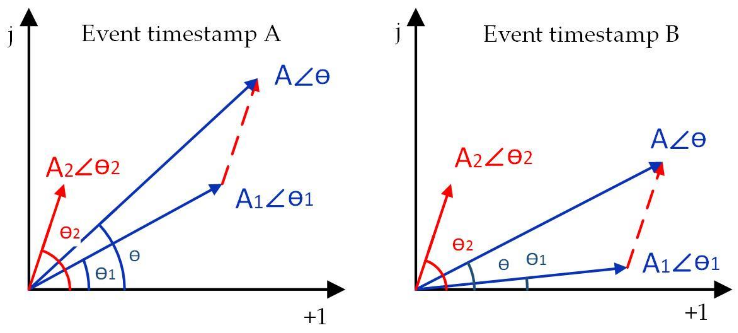
Figure 2.
Verification of the good additive property of U-I trajectory features (orange yellow plots are the U-I trajectories, dark blue plots are voltage waveforms and red plots are current waveforms) (a) waveforms and U-I trajectory of hairdryer; (b) waveforms and U-I trajectory of LED lamp; (c) waveforms and U-I trajectory of hairdryer and LED lamp working simultaneously; (d) waveforms and U-I trajectory of hairdryer by subtracting waveforms of LED lamp from that of hairdryer and LED lamp working simultaneously; (e) waveforms and U-I trajectory of LED lamp by subtracting waveforms of hairdryer from that of hairdryer and LED lamp working simultaneously; (f) waveforms and U-I trajectory of hairdryer and LED lamp working simultaneously by adding waveforms of hairdryer with that of LED lamp.

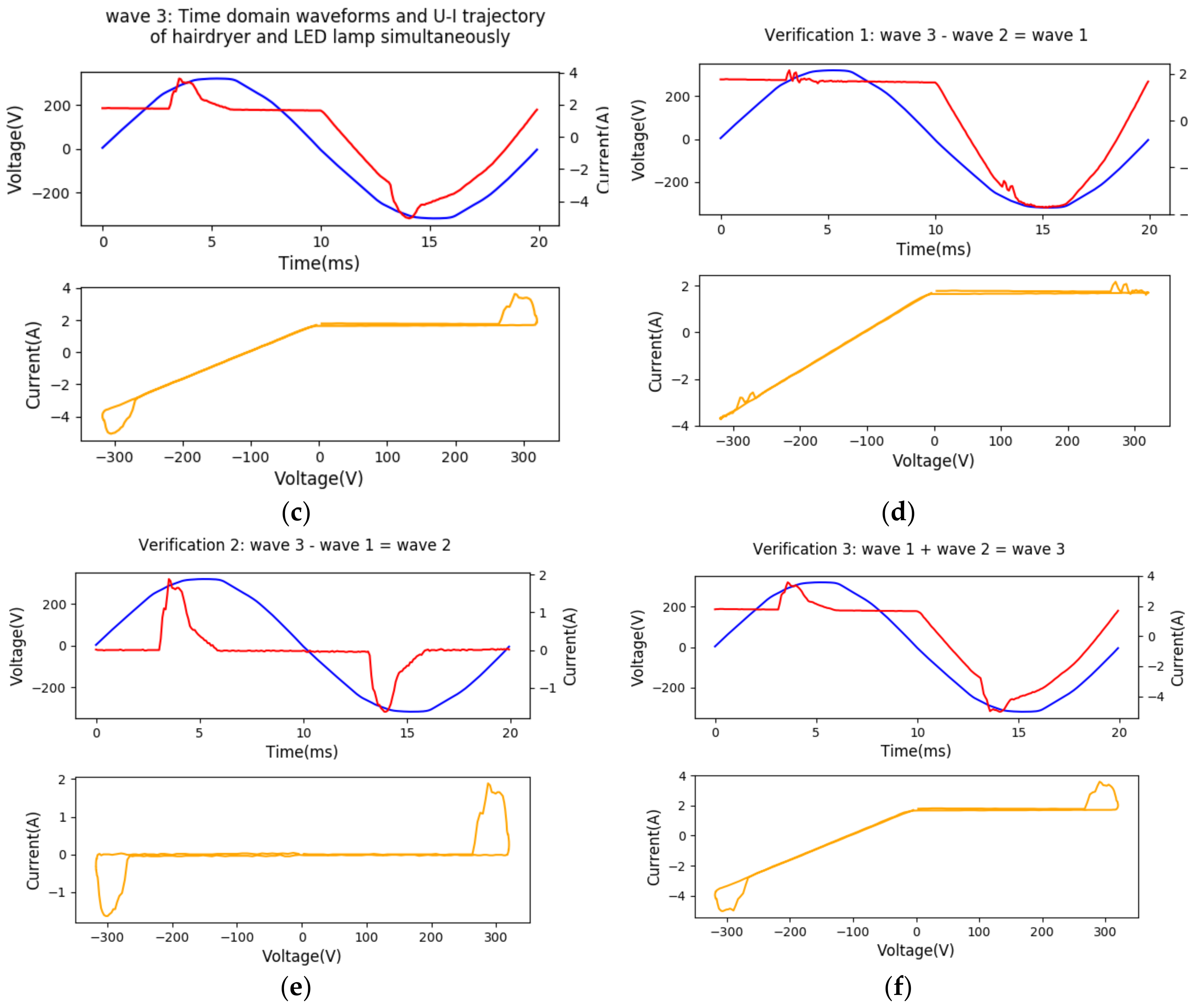
Figure 3.
The flow chart of proposed event-based NILM approach.

Figure 4.
Illustration of DBSCAN clustering based event detection algorithm.
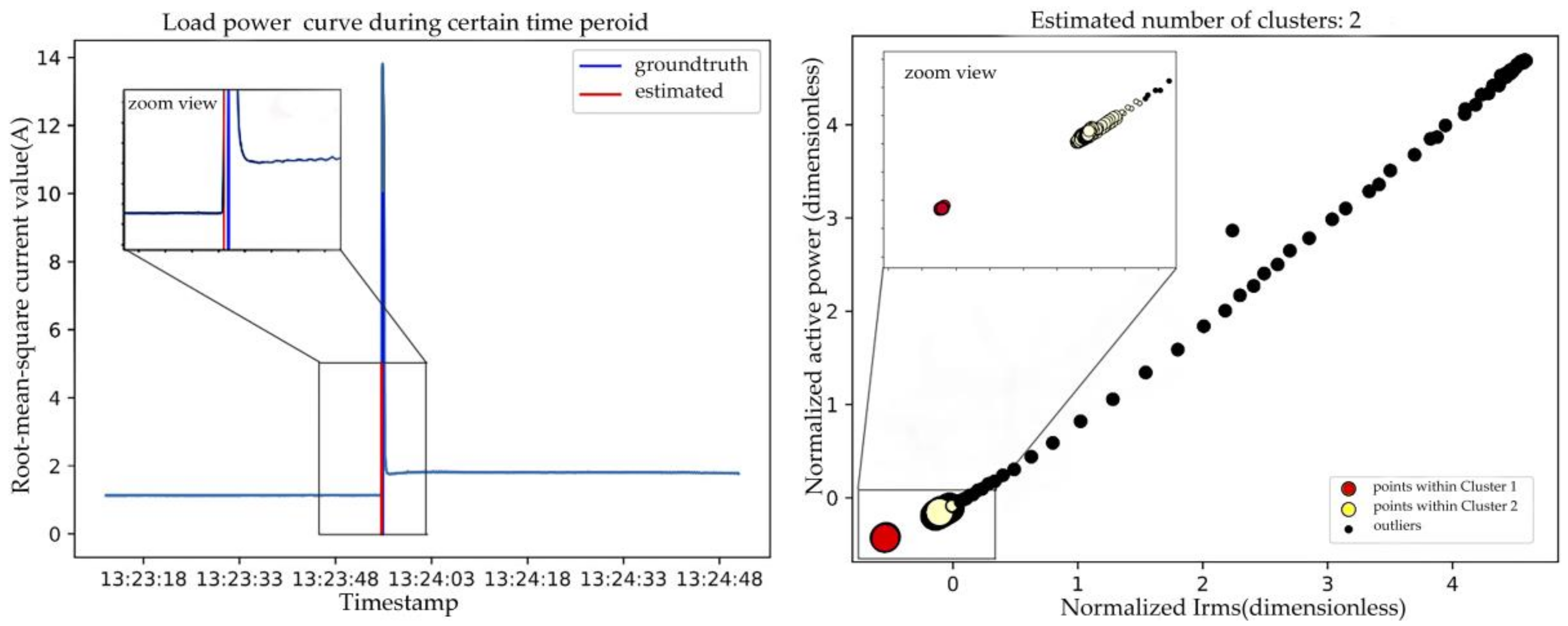
Figure 5.
The generation of clusters in DBSCAN clustering.

Figure 6.
Block diagram of the DBSCAN clustering based event detector.
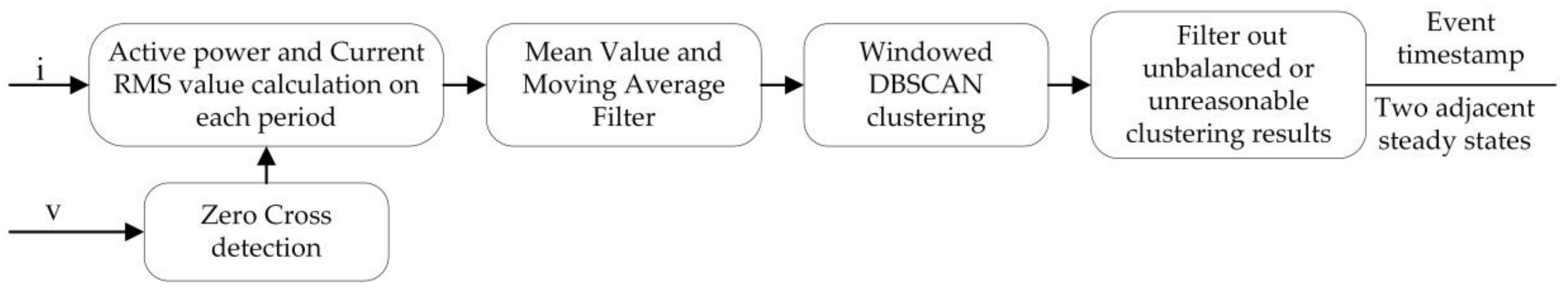
Figure 7.
Block diagram of event classification model based on harmonic current features.
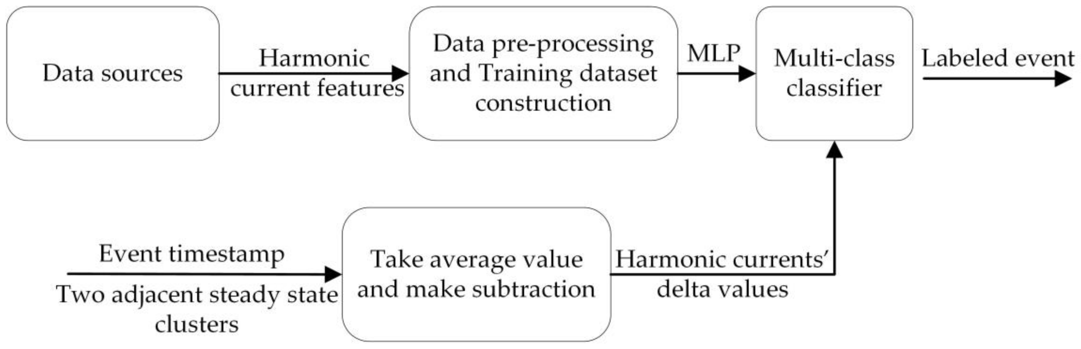
Figure 8.
MLP structure for event classification.

Figure 9.
Illustration of American three-wire two-phase electricity distribution network.

Figure 10.
Illustration of some events undefined in BLUED dataset.

Figure 11.
MLP classifier’s performance on PLAID dataset based on harmonic features (‘CFL’ and ‘ILBulb’ are short of ‘compact fluorescent lamp’ and ‘incandescent lightbulb’, respectively).
Figure 11.
MLP classifier’s performance on PLAID dataset based on harmonic features (‘CFL’ and ‘ILBulb’ are short of ‘compact fluorescent lamp’ and ‘incandescent lightbulb’, respectively).
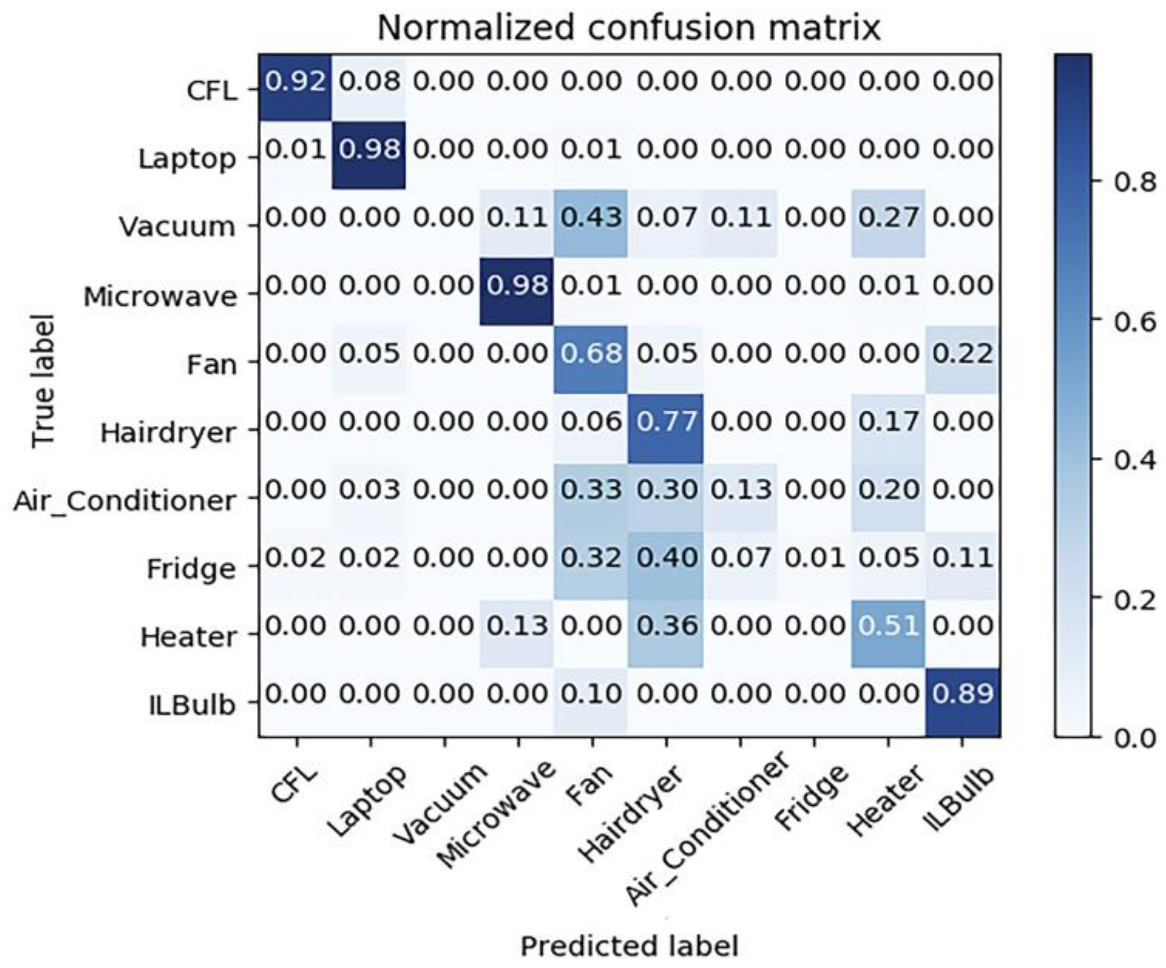
Figure 12.
Typical current and voltage waveforms of nine types of appliance.
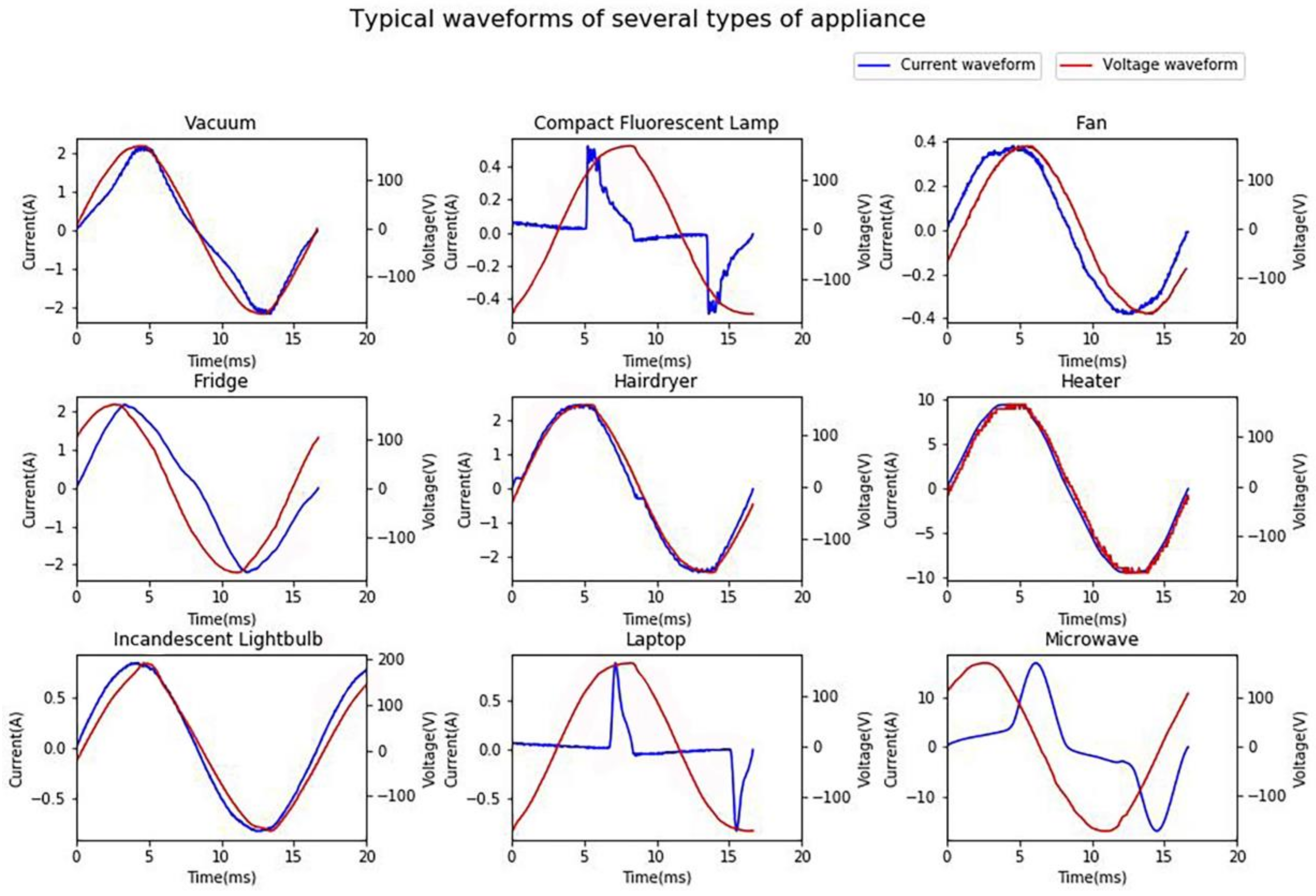
Figure 13.
K-fold cross-validation results of selected classifier: (a) normalized confusion matrix; and (b) ROC curve for multi-class classification (in Figure 13a and Figure 15, Hairdryer (H) denotes the hairdryers with half waveforms during on-state; Hairdryer (F) denotes the hairdryers with full waveforms; and CFL denotes compact fluorescent lamps).

Figure 14.
Classifiers’ performance increases linearly with the orders of harmonic currents.
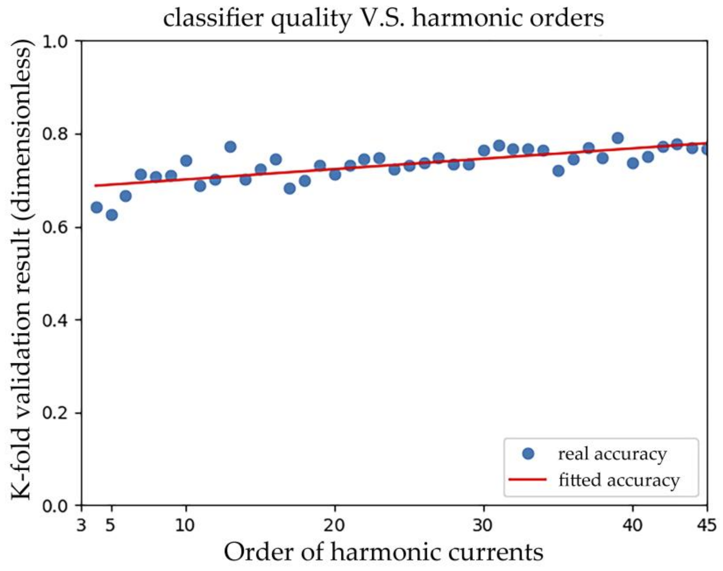
Figure 15.
Appliances’ work schedule in the laboratory: (a) Ground truth baseline; and (b) testing result (in Figure 13a and Figure 15, Hairdryer (H) denotes the hairdryers with half waveforms during on-state; Hairdryer (F) denotes the hairdryers with full waveforms; and CFL denotes compact fluorescent lamps).
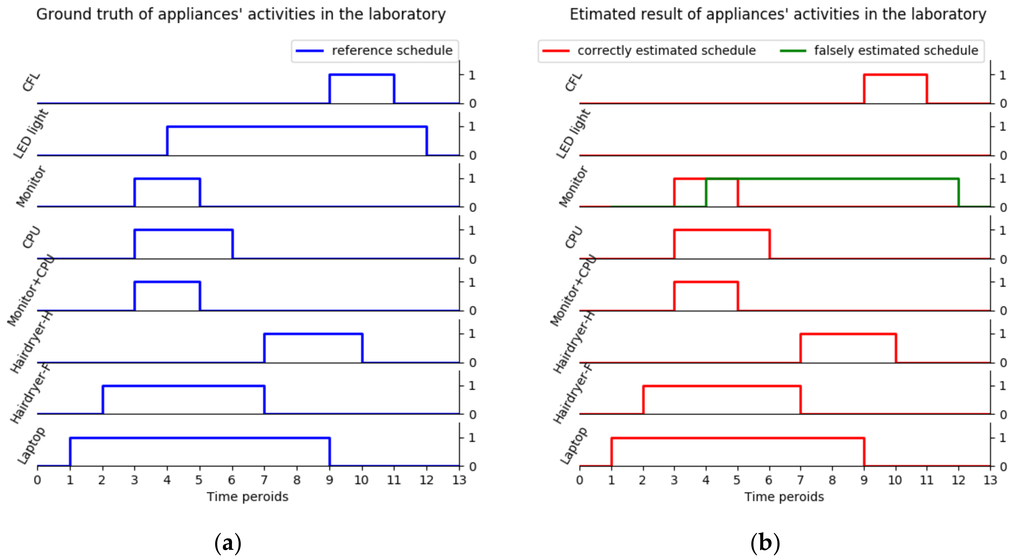

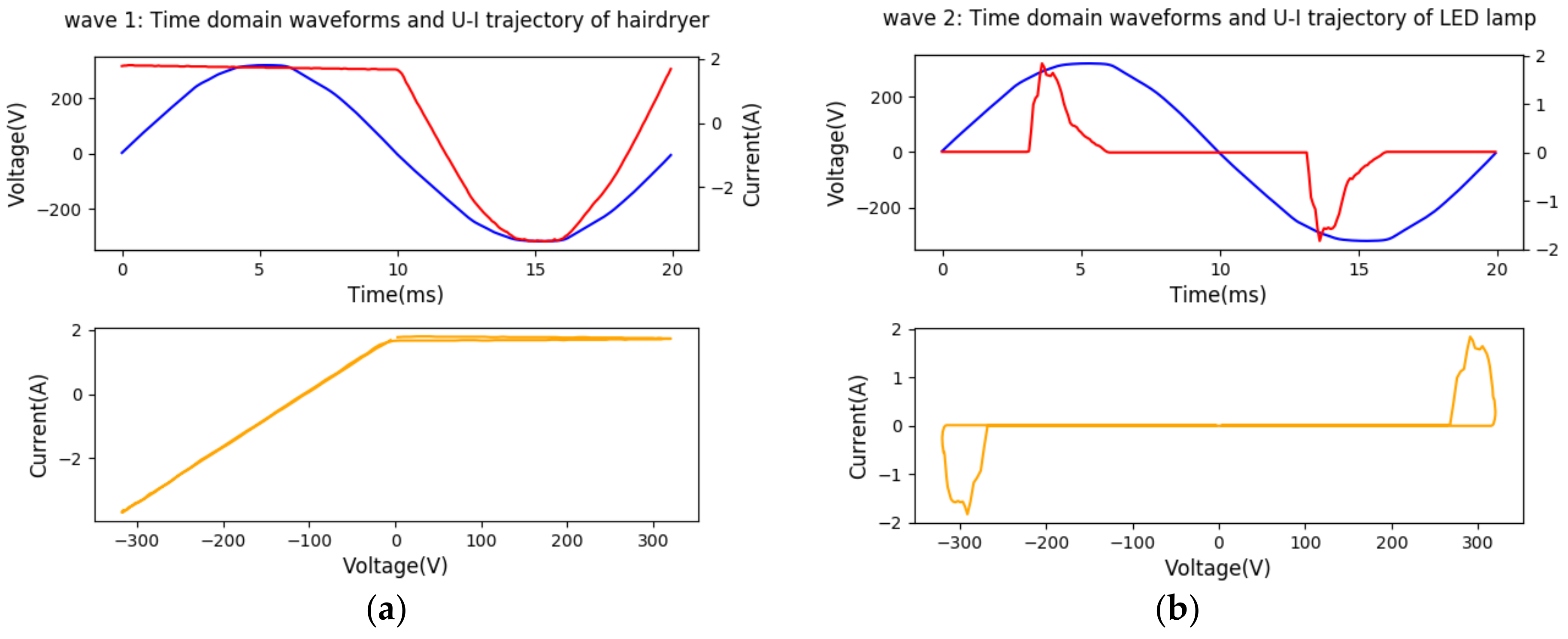
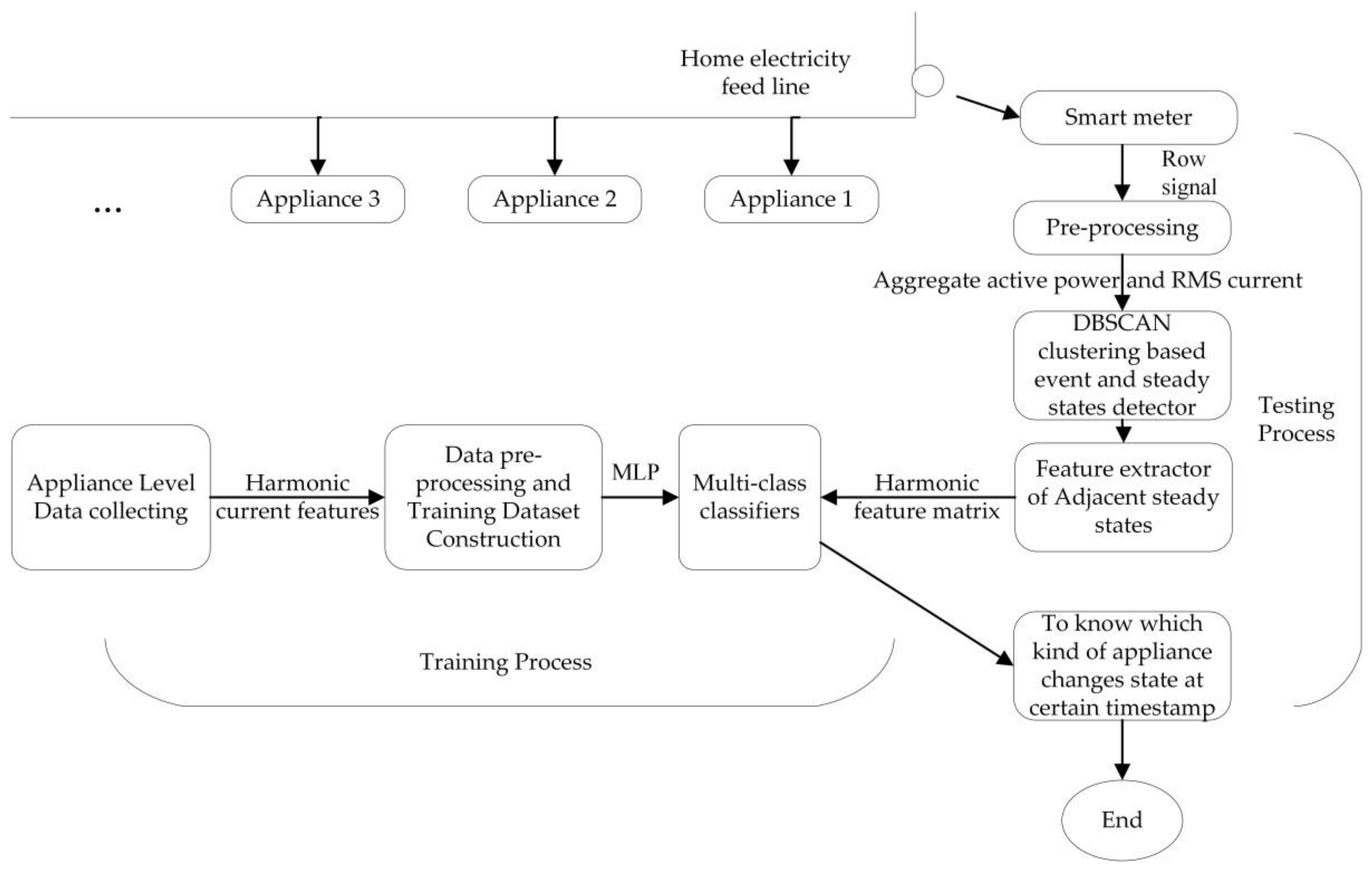
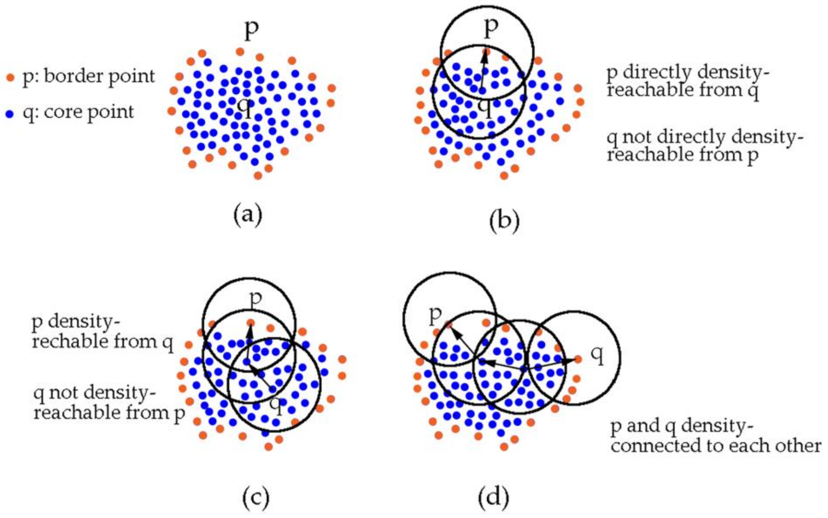
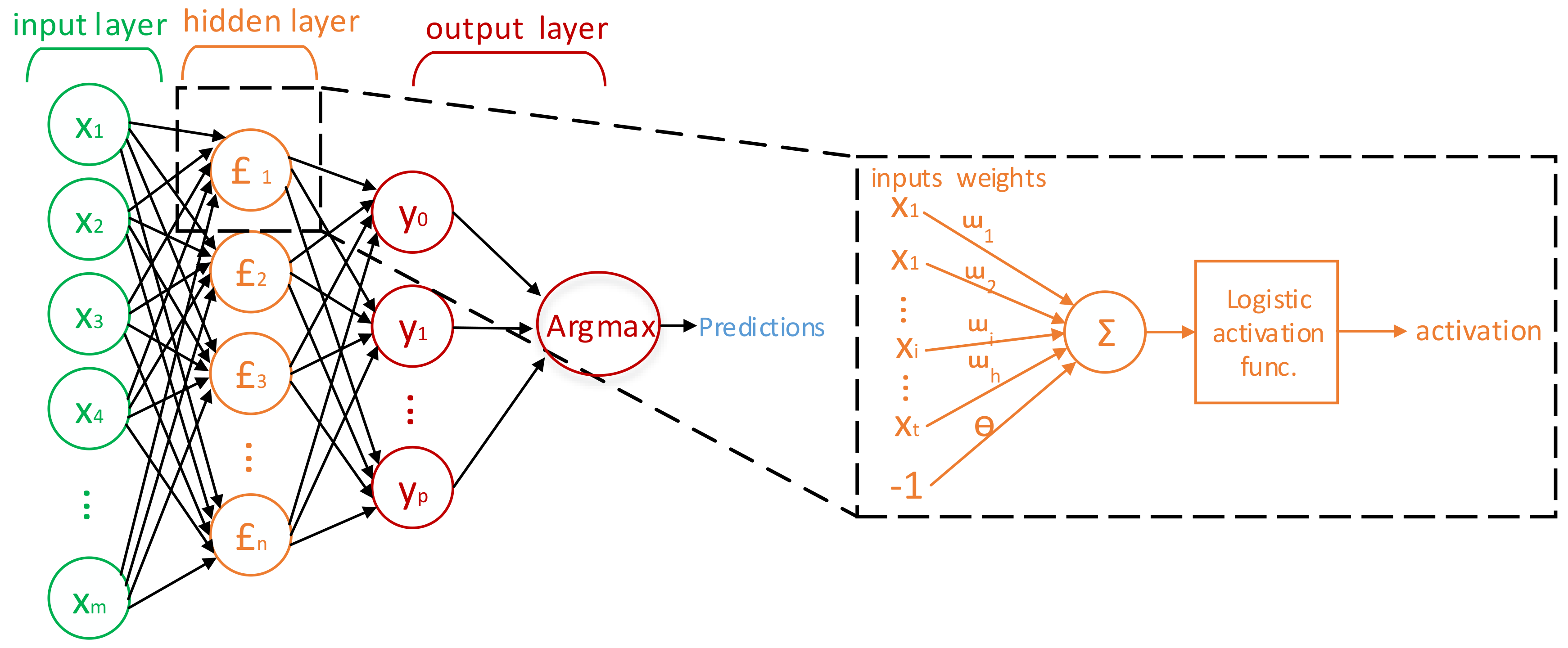
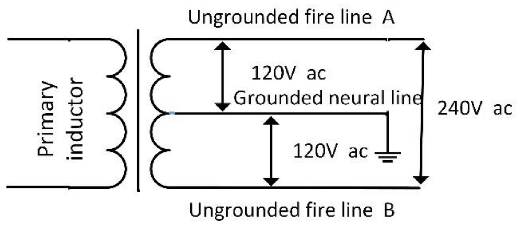
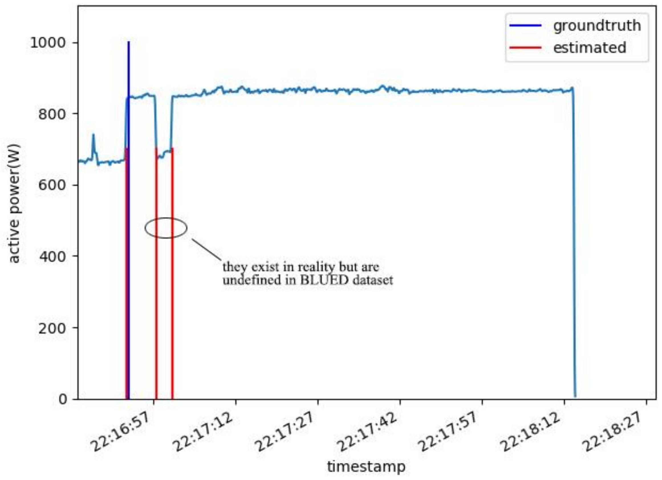
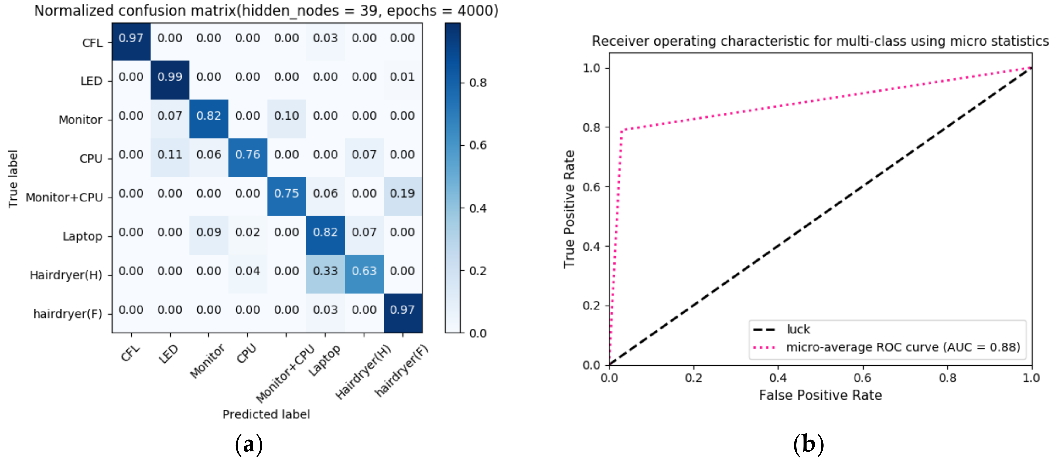
Table 1.
Verification of additive property of harmonic features and non-additive property of power quantities.
Table 1.
Verification of additive property of harmonic features and non-additive property of power quantities.
| Transition | 3rd Harmonic Quantity | Power Quantities Calculated by Equation (2) [23] | Power Quantities Calculated by Equation (3) | |||||||
|---|---|---|---|---|---|---|---|---|---|---|
| I3rd/A | θ/degree | S/VA | P/W | Q/Var | D/VA | S/VA | P/w | Q/Var | D/VA | |
| Null + (4) | 1.94 | −2.84 | 490.03 | 445.49 | −22.07 | 202.94 | 491.24 | 446.59 | −22.12 | 203.44 |
| (1) + (4) | 1.93 | −3.09 | 470.90 | 445.10 | −23.98 | 169.58 | 491.07 | 446.25 | −24.10 | 203.54 |
| (1)(2) + (4) | 1.93 | −3.08 | 442.61 | 444.43 | −23.81 | 125.44 | 488.78 | 445.28 | −23.92 | 200.13 |
| (1)(2)(3) + (4) | 1.94 | −3.17 | 435.11 | 446.79 | −24.66 | 113.32 | 491.59 | 448.00 | −24.81 | 200.85 |
Table 2.
Training dataset built by CW500 in the laboratory and its properties.
| Appliance Type | States Number | Instance Number | Records Number in Training Dataset |
|---|---|---|---|
| Compact Fluorescent light | 2 | 11 | 11 × 10 |
| LED lamp | 2 | 9 | 9 × 10 |
| Monitor | 2 | 9 | 9 × 10 |
| CPU | 2 | 7 | 7 × 10 |
| Monitor + CPU | 2 | 6 | 6 × 10 |
| Laptop | 2 | 7 | 7 × 10 |
| Hairdryer | 3 | 8 (half-wave) | 8 × 10 |
| 8 (full-wave) | 8 × 10 | ||
| Total records | 650 |
Table 3.
Harmonic decomposition accuracy.
| Harmonics/Order | Prime | 2nd | 3rd | 4th | 5th | 6th | 7th | 8th | 9th | |
|---|---|---|---|---|---|---|---|---|---|---|
| Reference | Amplitudes/V | 310 | 1.55 | 9.3 | 1.24 | 15.5 | 0.93 | 6.2 | 0.62 | 3.1 |
| Phases/degree | 2 | 9 | 18 | 38 | 68 | 98 | 178 | 248 | 350 | |
| Estimated | Amplitudes/V | 310.00 | 1.55 | 9.30 | 1.24 | 15.50 | 0.93 | 6.20 | 0.62 | 3.10 |
| Phase/degree | 2.00 | 9.25 | 18.00 | 37.87 | 68.00 | 98.07 | 178.00 | 248.02 | 350.00 | |
| Error | Amplitude/% | 0.00% | −0.10% | 0.00% | 0.01% | 0.00% | −0.04% | 0.00% | 0.00% | 0.00% |
| Phase/% | 0.01% | −2.79% | 0.02% | 0.33% | 0.00% | −0.07% | 0.00% | −0.01% | 0.00% | |
Note: “%” in last two rows means “percentage”, dimensionless.
Table 4.
Different event detection algorithms’ performance on BLUED dataset (Phase A).
| Algorithm | N(ref) | N(sys) | TP | FP | FN | FPR | TPR | P | F1 | TPP | FPP | AUC |
|---|---|---|---|---|---|---|---|---|---|---|---|---|
| DBSCAN Clustering | 846 | 841 | 835 | 6 | 11 | NA 1 | 98.70% | 99.29% | 98.99% | 98.70% | 0.71% | NA |
| GLR detector | 871 | 873 | 855 | 18 | 16 | NA | 98.16% | 97.94% | 98.05% | 98.16% | 2.07% | NA |
| Bucketing clustering | 886 | NA | NA | NA | NA | NA | NA | NA | NA | 98.50% | 0.55% | NA |
| Threshold filtering | NA | NA | NA | NA | NA | 0.09% | 94.00% | NA | NA | NA | NA | 97.00% |
Table 5.
Different event detection algorithms’ performance on BLUED dataset (Phase B).
| Algorithm | N(ref) | N(sys) | TP | FP | FN | FPR | TPR | P | F1 | TPP | FPP | AUC |
|---|---|---|---|---|---|---|---|---|---|---|---|---|
| DBSCAN Clustering | 1498 | 1914 | 1316 | 598 | 182 | NA | 87.85% | 68.76% | 77.14% | 87.85% | 39.92% | NA |
| GLR detector | 1551 | 1251 | 1092 | 159 | 459 | NA | 70.41% | 87.29% | 77.94% | 70.41% | 10.25% | NA |
| Bucketing clustering | 1579 | NA | NA | NA | NA | NA | NA | NA | NA | 70.50% | 8.75% | NA |
| Threshold filtering | NA | NA | NA | NA | NA | 12.00% | 88.00% | NA | NA | NA | NA | 0.94 |
1 “NA” means “not available”.
Table 6.
Average current total harmonic distortion rate of different appliance types.
| Appliance Type | CFL 2 | Laptop | Vacuum | Microwave | Fan | Hairdryer | Air Conditioner | Fridge | Heater | Lightbulb |
|---|---|---|---|---|---|---|---|---|---|---|
| Aver_THD 1 | 123.1% | 132.3% | 18.3% | 43.3% | 7.5% | 13.8% | 7.7% | 8.3% | 5.8% | 2.9% |
1 Average current total harmonic distortion rate, percentage, dimensionless; 2 compact fluorescent lamps.
Table 7.
K-fold cross-validation result of classifiers with different nodes number and fixed epochs number of 3000.
Table 7.
K-fold cross-validation result of classifiers with different nodes number and fixed epochs number of 3000.
| Hidden Layer Nodes # | K-Fold Result |
|---|---|
| 31 | 0.834391654 |
| 33 | 0.819818825 |
| 35 | 0.769962583 |
| 37 | 0.781195444 |
| 39 | 0.854912751 |
| 40 | 0.832755472 |
Table 8.
K-fold cross-validation result of classifiers with different epochs number and fixed nodes number of 39.
Table 8.
K-fold cross-validation result of classifiers with different epochs number and fixed nodes number of 39.
| Epochs # | K-Fold Result |
|---|---|
| 1000 | 0.700936276 |
| 2000 | 0.793135258 |
| 3000 | 0.854912751 |
| 4000 | 0.893898324 |
| 5000 | 0.862422104 |
| 6000 | 0.863903215 |
Table 9.
The computational complexity of DBSCAN clustering event detector and MLP classifier.
| Algorithms | Time Complexity (Big O Notation) | Space Complexity (Big O notation) | Experiment |
|---|---|---|---|
| DBSCAN clustering event detector; (N denotes the number of input points in one clustering) | Time consumed for each clustering is 8 ms; RAM space is neglected. | ||
| MLP classifier with three layers; (N denotes the nodes number) | Training time is 2.35 s; Classification time for one event is 6.7 ms; RAM Space is less than 1 MB |
© 2018 by the authors. Licensee MDPI, Basel, Switzerland. This article is an open access article distributed under the terms and conditions of the Creative Commons Attribution (CC BY) license (http://creativecommons.org/licenses/by/4.0/).
Share and Cite
MDPI and ACS Style
Zheng, Z.; Chen, H.; Luo, X. A Supervised Event-Based Non-Intrusive Load Monitoring for Non-Linear Appliances. Sustainability 2018, 10, 1001. https://doi.org/10.3390/su10041001
AMA Style
Zheng Z, Chen H, Luo X. A Supervised Event-Based Non-Intrusive Load Monitoring for Non-Linear Appliances. Sustainability. 2018; 10(4):1001. https://doi.org/10.3390/su10041001
Chicago/Turabian StyleZheng, Zhuang, Hainan Chen, and Xiaowei Luo. 2018. "A Supervised Event-Based Non-Intrusive Load Monitoring for Non-Linear Appliances" Sustainability 10, no. 4: 1001. https://doi.org/10.3390/su10041001
Note that from the first issue of 2016, this journal uses article numbers instead of page numbers. See further details here.