1. Introduction
Climate change, the volatility of crude oil prices, the issue of food security, and the global economic crisis have motivated decision-makers, industries, and economic agents involved in the biofuel sector to expand the use and production of biofuels [
1]. However, persistent low crude oil prices since 2014 seem to be an impediment to this effort.
The expansion of biofuels has established interlinkages between energy markets and agricultural markets given that corn is used to produce biofuels and soybean is used to produce biodiesel [
2].
The major objectives of a national policy for a healthy economy are food security, limitations on GHG emissions, economic growth, and compliance with objectives set by the Kyoto protocol. The biofuel market is an artificial market, the function of which is regulated by state [
3,
4]. The role of this market has become crucial in economic growth, satisfying the priority of sustainability. On the other hand, the alternative use of agricultural products such as corn and soybean (either for food or to produce biofuels) is leading to indirect land use change and to a deterioration in the problem of climate change.
Therefore, given the use of the two agricultural products in the production of biofuels, as well as their use for food, the existing mutual interdependencies reflect the mutual market interdependencies. Increasing prices of corn may well be attributed to the dominant conditions in the food market that are also providing an indication for the interdependency of corn price with biofuels [
5]. The specific relationship is related to many factors including the country, the model, and the dimension of time [
6].
On the other hand, given that corn and soybean evolved into a major motor-fuel energy source, a close relationship between corn (the major feedstock for ethanol) and soybean production (major input in biodiesel) with crude oil, the main feedstock for gasoline production, may be an expected result. The data used extends from late 2004 through mid-2008, when rapid expansion of the ethanol industry was occurring, which is the reason for which the relationship has been mainly established [
2,
7].
Most of issues mentioned above are reflected in the futures prices formatted on the NY stock exchange. A study on the co–movement of futures prices of agricultural products used especially in the production of bioenergy would be of great interest, while the role of crude oil prices seems to have had a great impact on those prices. Natanelov et al. [
8] have made a similar effort, and, according to their results, co-movement is a dynamic concept, and economic and policy development may affect the relationship between commodities, while they have also shown that biofuel policy has a strong impact in the co-movement of crude oil and corn futures until the crude oil prices surpass a certain threshold.
The concept of excess co-movement among futures prices has been subject to extended study with the assistance of different methodologies. The most widely used methodology is cointegration implemented for different time periods and providing conflict results (Pindyck and Rodenberg [
9], Natanelov et al. [
8]). Confirmation of co-movement is based on the herd behavior of financial prices [
9]. Ali et al. [
7], with the assistance of the partial equilibrium model, attributed the behavior of the commodity prices to specific demand and supply conditions. On the other hand, Natanelov et al. [
8] focused on price movements between crude oil futures and a series of agricultural commodities and gold futures by employing a comparative framework to identify changes in relationships over time. According to their findings, co-movement is validated as a dynamic concept, while policy development may reform the relationship between commodities and their determinants that are studied, that is, crude oil prices.
The present study is timely, given the particularities in the evolution of crude oil prices within the last few years. To be more specific, the global economic crisis led to extremely high values of crude oil prices in 2010, while since 2014 the crude oil prices have tended to be persistently low, a fact that may well lead to a high level of carbon emissions and limited substitution with renewable energy prices. The volatility of crude oil prices has a different impact in the short term rather than in the long term. In addition, a strand of literature developed on this specific issue focuses on the fact that the crude oil market has significant volatility spillover effects on non-energy commodity markets, which demonstrates its core position among commodity markets [
10]. This impact and its implications for the substitution of crude oil with other renewable or non–renewable resources seems to affect the level of carbon emissions and vice versa [
11].
Furthermore, the futures prices for each commodity reflect the market condition, as well as the agricultural policies implemented concerning their production, market conditions, assistant aid, or even energy policy that promotes their use to produce biomass.
The innovation of our study stands on the fact that we employ ARDL bounds cointegration to test the crude oil–corn prices and soybean–crude oil prices. The structure of the present work is organized as follows;
Section 2 describes material and methods,
Section 3 provides a brief literature review,
Section 4 provides the results and a short discussion, and
Section 5 concludes.
2. Literature Review
The energy–agricultural market interlinkages have become a subject of extended study within the last decade. The global food crises in 2007/08 and 2010/11, as well as negative environmental and social impacts of promoting biofuels, have given governments second thoughts regarding the promotion of biofuels.
Since the outbreaks of biofuels industry, an abundance of manuscripts have focused on dependency between fossil fuel, biofuel, and feedstock prices [
12,
13,
14,
15]. In a few papers and due to data availability issues, the biofuel prices are ignored [
2]. In those studies, ignoring biofuel prices generally relies on the hypothesis that a change in the food–fuel price relationship post the outbreak of the biofuels industry is related to the impact of biofuels.
In most of these studies, the analysis used is cointegration and/or estimation of a VECM, or one of its generalized nonlinear versions. For the case of US, cointegration is validated between agricultural prices and energy prices, while energy prices are considered to drive the feedstock prices [
12,
16,
17] (Saghaian 2010; Serra et al. 2011a; Wixson and Katchova 2012). The works conclude that the interlinkages are attributed to the existence of biofuel markets. Only Zhang et al. [
14] confirm no evidence of cointegration between energy and agricultural commodity prices. Furthermore, only Serra et al. (2011) [
12] and Rajcaniova and Pokrivcak (2011) [
18] confirm that biofuel markets may shape fossil fuel prices.
In general, in most cases it is concluded that energy prices drive long-run world agricultural price levels [
2]. In global terms, Nazlioglu and Soytas [
19] appraise the link between world crude oil prices, USD exchange rates, and a long list of world agricultural commodity prices. In addition, Nazlioglu [
20] finds evidence of cointegration between corn, soybean, and wheat with oil prices, especially in recent years. In another work, Yu et al. [
21], focusing on the relationship between crude oil and edible oil prices, find no evidence of energy prices driving food prices.
The methodology of autoregressive distributed lag models (ARDL models) has been employed in many works [
22,
23,
24].
To be more specific, Cooke and Robles [
22] confirm that recent increases in world corn, wheat, rice, and soybean prices are strongly affected by oil prices. Chen et al. [
23] find evidence of positive short-run links between crude oil and grain prices, while Esmaeili and Shokoohi [
24] investigate co-movement of world food prices, oil prices, and different macroeconomic variables. According to their findings, crude oil prices affect food prices only indirectly through the food production index.
Global data, with a time period including peaks of crude oil prices and persistent low prices with the assistance of ARDL cointegration approach, and the futures prices that are considered more informative than real prices, constitute the innovation of the present manuscript.
3. Material and Methods
The data employed in the present work are monthly futures prices of crude oil (CME NYMEX WTI Crude Oil Futures in US dollars per ton), corn, and soybeans (CME CBOT grain futures), derived by Bloomberg [
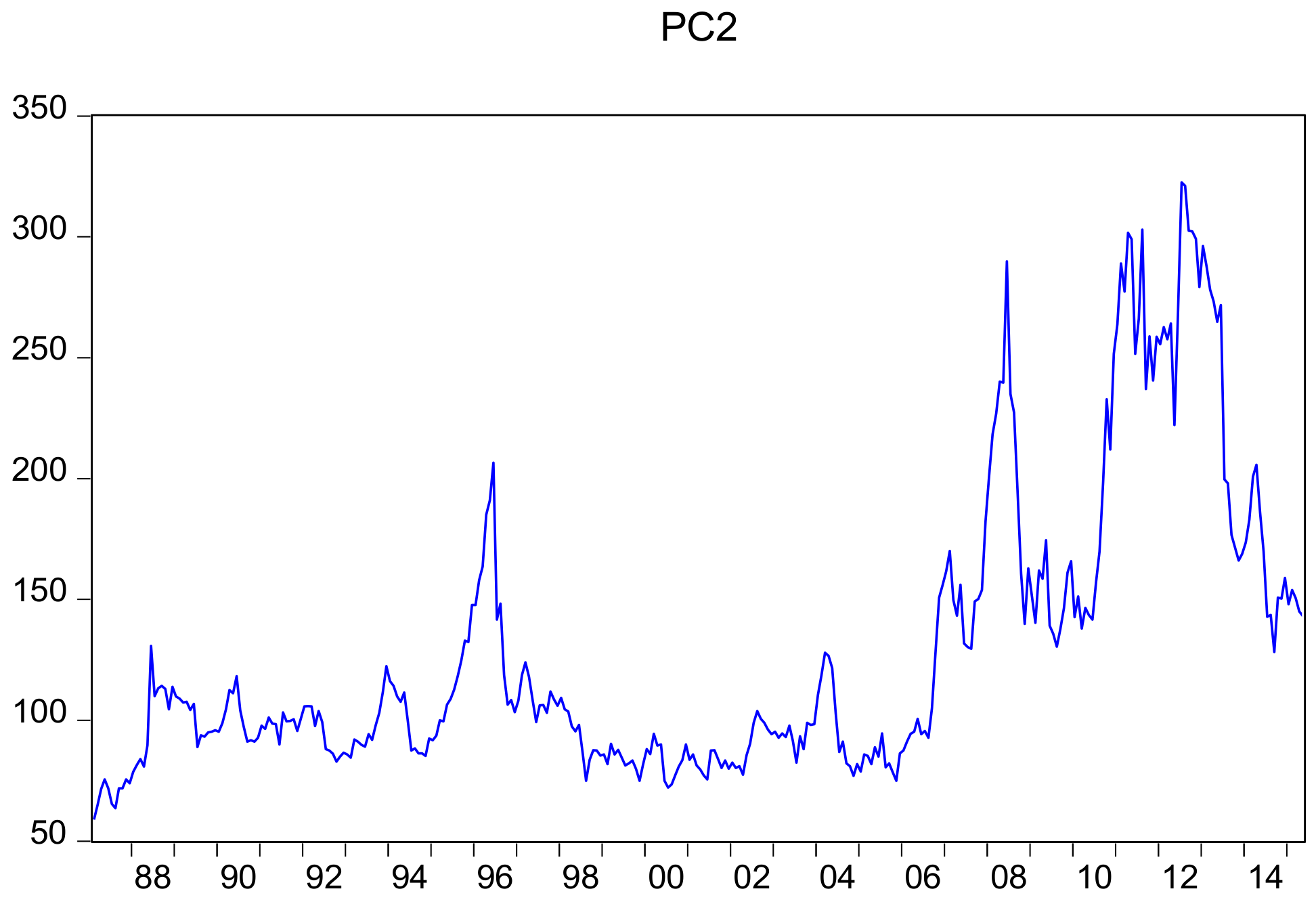
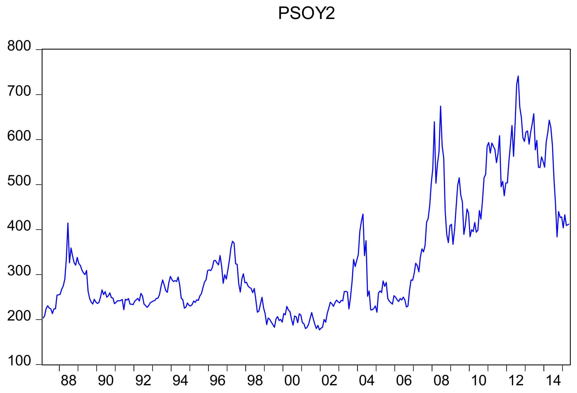
25]. The study period is from July 1987 until February 2015. To account for the problem of comparing disparate price units, the data is indexed based on the price of August 1999 for each commodity.
Trend analysis of the data used for empirical investigation on the selected variables can be seen in
Figure 1 and
Figure 2. To be more specific,
Figure 1 illustrates the evolution of futures prices of crude oil,
Figure 2 illustrates the evolution of corn futures prices, and, finally,
Figure 3 illustrates the evolution of soybean futures prices.
Evidently, an increasing trend is validated for the case of crude oil prices with two structural breaks observed in 1999 and 2008 that will be further investigated with the assistance of a break unit root test.
On the other hand, for the case of the corn futures prices,
Figure 2 presents a series of peaks that document the necessity of a break unit root test to examine the stationarity. Similar behavior can be seen for the case of soybean, since similar peaks are observed for the same time periods, as can be seen in
Figure 3.
3.1. Model Specification
We employed ARDL bounds cointegration process to estimate the relationship between the prices of the two agricultural commodities and crude oil prices. This relationship involves futures prices for soybean and corn, with crude oil prices as formatted in NY stock exchange. The advantage for the use of futures prices is that they represent not only the supply and demand conditions in the agricultural market but also a trend in the global economy (including economic crises, changes in exchange rates, etc.). Therefore, significant events that have an impact either on crude oil prices or on the agricultural commodities or changes in the major lines of energy policy (biofuels, issue of food security, and others) should be reflected in the estimated model in order for useful conclusions to come out.
The relationship to be examined for the case of corn is specified as follows:
In addition, in the case of soybean, the bivariate relationship to be surveyed is the following:
3.2. Theoretical Econometric Framework
The methodology implemented is the ARDL bounds cointegration, given the limited data available [
26]. Prior to the empirical investigation of co-movement among the variables under review with the assistance of ARDL cointegration approach, in order to check stationarity in the data, it is necessary to employ a unit root test. The unit root test used is the Augmented Dickey Fuller (ADF) break unit root test, given the structural breaks observed in the variables studied. The specific test involves a two-step procedure. In the first step the intercept, trend, and breaking variables are used to detrend the series with the assistance of ordinary least squares (OLS), and in the second step the detrended series are employed to test the existence of a unit root with the assistance of a modified Dickey-Fuller regression [
27]. The first model may involve non-trending data with intercept break, trending data with intercept break, trending data with intercept and trend break, and finally trending data with trend break. The results refer either the trend specification (trend, intercept, or both) or to the break specification (trend, intercept, or both).
The problem of selecting an appropriate method of unit root test may well lead to misspecifications. For that reason, in the present manuscript, we have adopted the sequential procedure proposed by Shrestha and Chowdhury [
28] in selecting the optimal method and model of the unit root test. The Shrestha-Chowdhury general-to-specific model selection procedure has been presented subtly in the work of Shrestha and Chowdhury [
28].
The main objective of the particular test is to ensure that the time series employed are not I(2), a condition that implies robustness for the results derived by the ARDL bounds cointegration test.
Having validated the existence of cointegration, we estimate the Unrestricted Error Correction Model (UECM). The lag selection through which the data generating process is captured is based on the general-to-specific framework [
29].
The ARDL model employed is, however, slightly modified in an appropriate way in order residual serial correlation and endogeneity problems to be corrected simultaneously [
30]. The following UECM is used for our purpose.
The ARDL model employed is modified in an appropriate way in order for residual serial correlation and endogeneity problems to be corrected simultaneously [
30]. The following UECM is used for our purpose.
in which
Yt demotes the dependent variable and
Xt denotes the independent variable in every individual case.
In Equation (3), we may identify the long term as well as the short-term parameters. To be more specific, β1 represents the long-term parameter while rejecting the null hypothesis, and β1 = 0 (equivalent to no cointegration) against the alternate, according to which β1 ≠ 0 (which implies that the variables are cointegrated), The test for cointegration is based on the computed F-statistic compared to the values of the tabulated critical bounds. The upper critical bound (UCB) is employed under the condition that the regressors are I(1) or I(0), while the lower critical bound is used only under the condition that they are I(0). The potential results of the test are the following:
- (1)
If the F statistic exceeds the Upper Critical Bound, cointegration is confirmed;
- (2)
In case the F statistic is less than the lower Critical Value, the null hypothesis of no cointegration is confirmed;
- (3)
An area of uncertainty is determined within the two critical bounds, a case in which our decision relies on the lagged error correction term for a long run relationship.
The validity of the existence of a long run relationship allows the estimation of the error correction model (short run dynamics are surveyed), for which also sensitivity test, parameter stability, and goodness of fit using cumulative sum of squares of recursive residuals (CUSUM) is implemented.
The error correction model estimated for each bivariate relationship examined for the variables under review is provided by Equation (4).
L denotes the lag operator, and ECM denotes the error correction term generated by the cointegrating equation, while the η terms are serially independent random error terms. The F statistic for the parameters of first differences validates the short run causality, while on the other hand the statistical significance of φi coefficients with the assistance of t statistics provides evidence for the long run causality.
4. Results–Discussion
According to our findings provided in
Table 1, with the assistance of a breakpoint ADF unit root test, all the variables employed are I(1), a result that allows us to bounds test.
The second stage in our methodology involves the bounds testing to confirm or reject cointegration. The results are provided in the following
Table 2.
The next
Table 3 provides the estimated results on the long run relationships.
According to our findings, the results derived indicate the existence of interactions among agricultural commodities and crude oil prices. This is an expected result, and it validates the interactions of agricultural markets and crude oil markets in global terms. The specific results are interpreted as follows: given that corn is the major input for ethanol, a substitute for crude oil prices, the behavior of crude oil prices may well reflect the behavior of corn prices. To be more specific, high crude oil prices lead to high ethanol prices and therefore higher corn prices. Conversely, decreases in crude oil price will lead to a lower gasoline price, a lower ethanol price, and a lower breakeven corn price.
Furthermore, the results derived should be free from misspecification and autocorrelation or heteroscedasticity of the residuals. For that reason, all the tests concerning specification, autocorrelation, and heteroscedasticity tests are presented in
Table 4. According to our findings, whiteness of the residuals for all the models, as well as no misspecification problems, were confirmed.
The next step in our analysis involves the presentation of the short run dynamics of the error correction model estimated in order to examine the interactions among the corn prices and the crude oil prices in the short run and to highlight the differences with the results derived in the long run. These results are provided in
Table 5 and
Table 6. According to our findings, the results are not different from those derived in the long run. To be more specific, in the short term crude oil prices do not seem to have a statistically significant impact on the formation of a future’s price of an agricultural product, i.e., corn. The return to the steady state is statistically significant, with a speed of 6% per month.
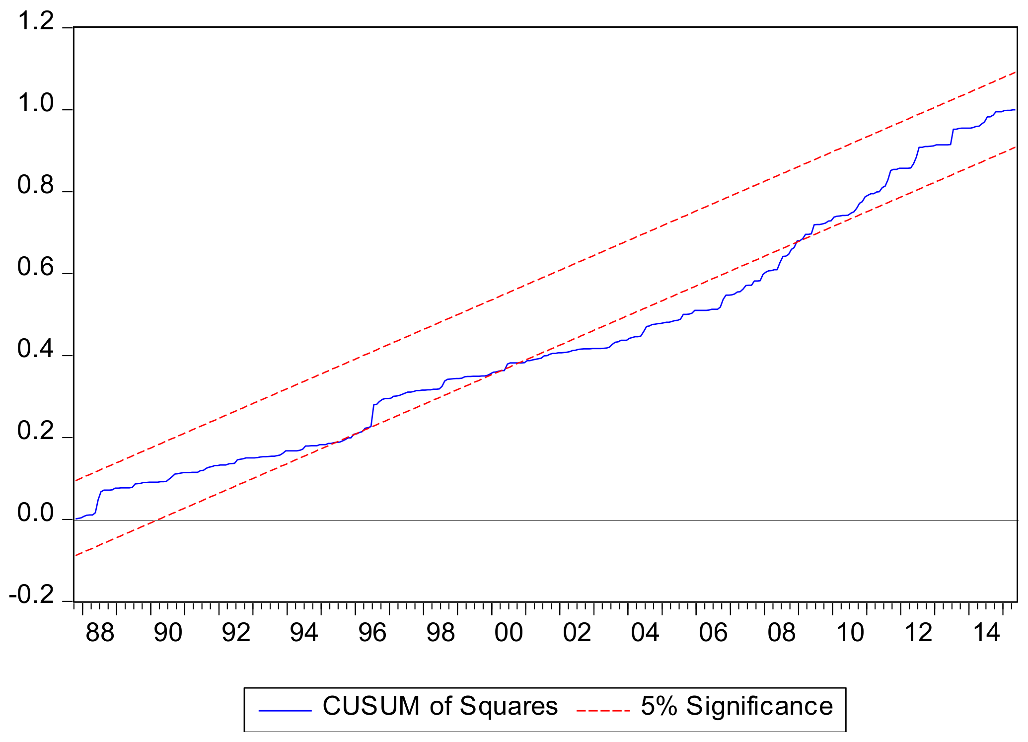
Regarding the last step in our analysis, the parameter stability of the estimated model is conducted with the assistance of the CUSUM of squared residual test.
Evidently, based on
Figure 4, the graph of the corn–crude oil prices remains partially between the lines, a result indicating limited stability of the estimated coefficients for the period studied.
On the other hand, for the case of soybean crude oil prices relationship as illustrated in
Figure 5, the CUSUM test of squared residuals confirms parameter stability.
Limited parameter stability is validated for the estimated model according to
Figure 5. The findings based on our data indicate a long run relationship for both bivariate relationships, though in the short run no relationship is validated. This is an expected result given that the interaction between energy and agricultural market has evolved in the long run and not in the short run. This result is in line with that of Natanelov et al. [
8], while the policies under the condition of the assumption of the long-run presence of a certain degree of linkage between energy markets and the market of food products that substitutes for other food products used as energy feedstock, and between food products used as energy feedstock and their substitutes for food exhibiting strong seasonality in production, would need to be flexible to be effective. The periodical shocks in the supply and demand of these agricultural commodities should be taken into consideration given that they may have a severe impact on the market interlinkages between different production periods.
The study of this relationship is important due also to the changes in biofuels industry. To be more specific, global biofuel production has been growing for the decade 2005–2015 with result that in the year 2014 ethanol production reached about 114 billion liters and biodiesel production reached about 30 billion liters [
31]. The implementation of biofuel policies in global terms can expand the use of biofuels leading to a reduction in greenhouse gas emissions, along with limitation in the dependency on fossil fuel.
Though the interlinkages with the agricultural markets have led to high food prices, the simultaneous increase in feedstock prices has been harmful for biofuel competitiveness in the liquid fuels market, necessitating the need for subsidization and other protectionist policies. The solution to this problem is the promotion of second generation biofuels for which no food crops are used, since it will limit the competition for agricultural land and crops, reducing in turn the impact on agricultural prices. A final implication of our findings (the impact of energy prices on feedstock prices) can provide the food policy makers with a tool to forecast food prices and implement food policies with regard to the evolution of energy prices.

 and
and 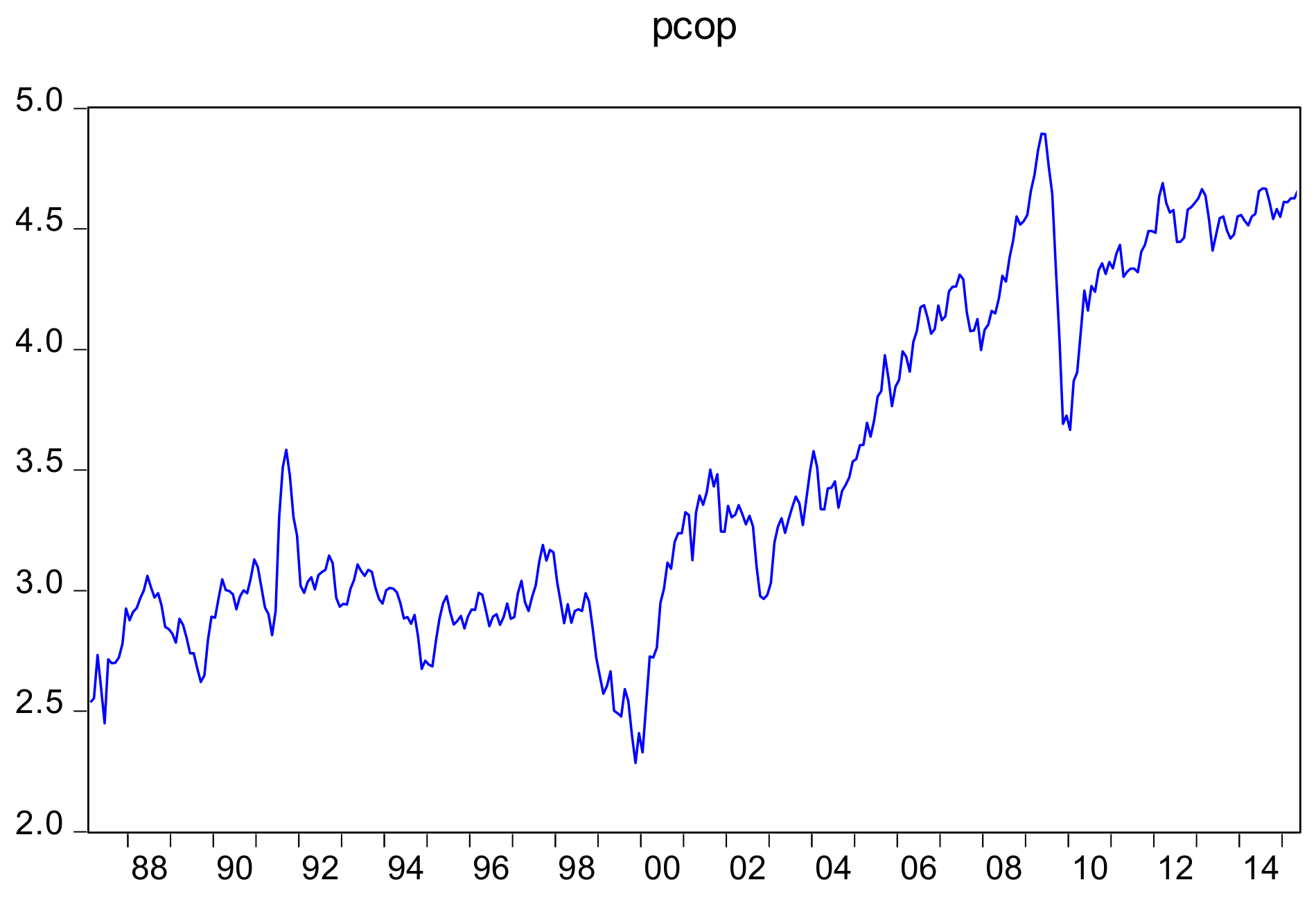


