Simulating and Predicting the Impacts of Light Rail Transit Systems on Urban Land Use by Using Cellular Automata: A Case Study of Dongguan, China

1
School of Geographical Sciences, Guangzhou University, Guangzhou 510006, China
2
Dongguan Geographic Information and Urban Planning Researching Center, Dongguan 523129, China
3
Baiyun District Planning and Resources Information Management Center, Guangzhou 510405, China
4
School of Geography and Planning, Guangdong Key Laboratory for Urbanization and Geo-simulation, Sun Yat-sen University, Guangzhou 510275, China
*
Author to whom correspondence should be addressed.
Sustainability 2018, 10(4), 1293; https://doi.org/10.3390/su10041293
Submission received: 24 March 2018
/
Revised: 20 April 2018
/
Accepted: 20 April 2018
/
Published: 23 April 2018
(This article belongs to the Section Sustainable Transportation)
Abstract
:The emergence of Light Rail Transit systems (LRTs) could exert considerable impacts on sustainable urban development. It is crucial to predict the potential land use changes since LRTs are being increasingly built throughout the world. While various land use and land cover change (LUCC) models have been developed during the past two decades, the basic assumption for LUCC prediction is the continuation of present trends in land use development. It is therefore unreasonable to predict potential urban land use changes associated with LRTs simply based on earlier trends because the impacts of LRT investment may vary greatly over time. To tackle this challenge, our study aims to share the experiences from previous lines with newly planned lines. Dongguan, whose government decided to build LRTs around 2008, was selected as the study area. First, we assessed the impacts of this city’s first LRT (Line R2) on three urban land use types (i.e., industrial development, commercial and residential development, and rural development) at different periods. The results indicate that Line R2 exerted a negative impact on industrial development and rural development, but a positive impact on commercial and residential development during the planning stage of this line. Second, such spatial impacts (the consequent land use changes) during this stage were simulated by using artificial neural network cellular automata. More importantly, we further predicted the potential impacts of Line R1, which is assumed to be a newly planned line, based on the above calibrated model and a traditional method respectively. The comparisons between them demonstrate the effectiveness of our method, which can easily take advantage of the experiences from other LRTs. The proposed method is expected to provide technical support for sustainable urban and transportation planning.
1. Introduction
In China, immoderate urban expansion has given rise to a series of social, ecological and environmental issues [1,2]. Numerous studies have indicated that the urban land area in this country exhibited an exponential growth pattern during the past two decades [3,4,5]. This unprecedented phenomenon is accompanied by massive rural-urban migration [6,7]. According to the National Population Census, the percentage of urban population in China grew from 36.22% to 49.68% between 2000 and 2010 [8]. As a consequence, this country has also witnessed an increase in private vehicle ownership and usage. Traffic congestion is gradually becoming one of the greatest obstacles to city development [9,10,11]. To alleviate these problems, Chinese governments have given a high priority to the investment in Light Rail Transit (LRT) systems [12,13]. For example, many LRTs have been put into operation in some large cities (e.g., Shanghai, Tianjin, Nanjing) over the last fifteen years [13,14,15].
The development of LRTs will inevitably exert substantial impacts on surrounding urban land use, both spatially and quantitatively [16,17,18,19,20,21,22]. For example, population relocation and economic development may be stimulated by the improved transport accessibility. It is crucial to simulate and predict the consequent spatio-temporal dynamics of land use if policy-makers decide to build a new line. However, previous studies mainly focused on the impacts of LRT investment on land and property values [23,24,25,26,27,28,29]. Some others have analyzed the impacts on labor market, crime rate, and public discourse [30,31,32,33,34]. Less effort has been made to simulate and particularly predict the potential urban land use changes associated with the development of LRTs. Urban landscape planning has many benefits in terms of the environment. Urban landscape planning means making decisions about the future situation of urban land [35]. In this case, it is necessary to predict how the land has changed over time and the effects of natural factors and human activities on the land [36]. In this way, successful and sustainable landscape planning studies can be achieved. Recently, Joshi et al. [37] simulated the impacts of LRT on urban development by using UrbanSim model; Basse [38] proposed a cellular automaton (CA) model for simulating the impacts of high-speed rail on land use dynamics; and Aljoufie et al. [39,40] developed a CA-based land use and transport interaction model.
Nevertheless, it remains a tough challenge to better predict potential spatial impacts of LRTs. While various land use and land cover change (LUCC) models have been developed for geo-simulation applications during the last twenty years [41,42,43,44,45,46,47,48,49], the basic assumption for LUCC prediction is the continuation of present trends and dynamics of land use change into the future [50,51]. Unfortunately, the impacts of LRT development will vary considerably over time [18,23], which adds more complexity to the evolution of land use. To better handle this problem, our study attempts to share the experiences from a previous line with newly planned lines by using an artificial neural network CA model, which has been widely employed for modeling multiple land use changes (e.g., [50,52,53]). Specifically, the model parameters calibrated based on previous lines could be reused to predict potential urban land use changes influenced by new lines. Dongguan is one of the biggest manufacturing bases in China. The investment in LRTs has become an urgent task for the local government due to a massive influx of population [54]. As a result, this city is an appropriate case through which we can evaluate the proposed method.
2. Methodology
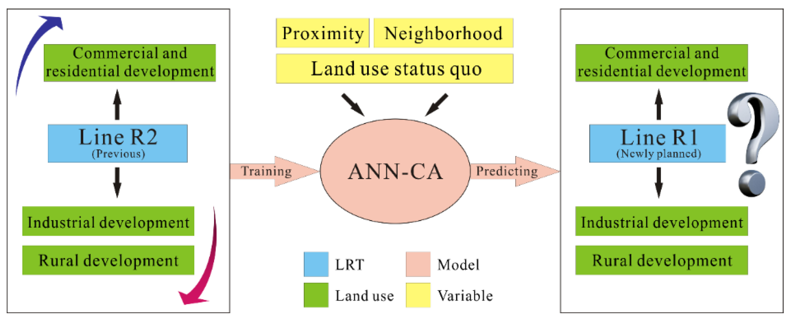
In this study, a methodology is developed to provide a modeling framework which can reuse the experiences from Dongguan’s first LRT (Line R2) for the analysis of a new LRT (Line R1). To do so, we will first assess the impacts of R2 on its surrounding urban land use over different periods with the support of buffer operations. Then, the spatial dynamics of land use within a 2 km two-sided buffer from 2008 to 2011 (the planning stage of R2) will be simulated by using an artificial neural network cellular automata model.
More importantly, the spatial impacts of Line R1 on its surrounding urban land use during the same stage can be predicted based on the experiences drawn from Line R2 (i.e., the above calibrated model). The flowchart of this study is illustrated in Figure 1.
2.1. Assessing the Impacts of LRTs on Surrounding Urban Land Use
The development of Light Rail Transit systems (LRTs) can be divided into four stages, namely the pre-planning, planning, construction, and operation stages [18,23,55]. Time series of remote sensing images are helpful for monitoring land use changes over different periods. However, it may be difficult to identify detailed urban land use types (e.g., industrial or commercial development) from the widely used Landsat Thematic Mapper (TM) images since the spatial resolution is only 30 m. Therefore, Système Probatoire d’Observation de la Terre (SPOT) images, which have a much finer resolution of 2.5 m, are used in this study. To assess the impacts of LRT development on surrounding urban land use, we also need to build a two-sided buffer because LRTs mainly exert impacts on land use within a certain proximity [23,24,26]. Previous studies related to the cases in Chinese cities have indicated that a 2 km buffer is quite suitable for quantifying the LRT impacts on land use [13,14,55]. Nevertheless, such impacts may vary significantly across regions, economic zones, and policy regime, and we should analyze the gradual transition of land use changes to better determine the buffer size. Although this study mainly focuses on the land use changes within a designated buffer, the applicability of the proposed modeling framework still remains unchanged if the buffer varies. Then, land use transition matrix will be used for land use change detection within the buffer, while the change trends of each land use type over different stages can be directly compared by using the following equation [56]:
where K denotes the rate of land use changes during a certain period, Ua and Ub denote the area of one land use type at the beginning and the end of the period respectively, and T denotes the length of the period (in years).
2.2. Modeling Land Use Changes by Artificial Neural Network Cellular Automata
The simulation and prediction of multiple land use changes are tough tasks given the complex non-linear relationships of land use conversion. To deal with this problem, Li and Yeh [50] proposed an artificial neural network cellular automaton (ANN-CA) model, which is an iterative integration of artificial neural network and CA. At each iteration, CA will simulate spatial dynamics of land use based on the land use conversion probabilities generated by the network. Since ANN-CA is a useful tool for modeling multiple land use changes [50], it is selected in our study to simulate and predict the spatio-temporal changes of industrial development, commercial and residential development, and rural development.
In general, an ANN consists of three layers, namely input, hidden, and output layers. The first layer contains m neurons that respectively represent m different spatial variables related to urban land use dynamics. The number of neurons in the hidden layer could be set as 2m/3 [50], while the output layer has n neurons. Each output neuron provides a conversion probability corresponding to one land use type. The network can be trained based on the well-known back propagation learning method [57]. The detailed procedures are introduced as follows [50]:
First, a study area should be represented by a two-dimensional matrix since CA are cell-based models. Each cell (i.e., matrix element) has m attribute values corresponding to m spatial variables. These site attributes, which will serve as the inputs to the first layer of an ANN, determine the direction of land use conversion. They can be formulated as follows:
where is the ith attribute value for cell k at time t, and T denotes transposition.
Then, the signals received by the hidden layer can be calculated by using the following equation:
where is the signal transmitted from cell k at time t to the hidden layer’s jth neuron, and is the parameter between the input and hidden layers. The hidden layer will subsequently make responses by using a sigmoidal function:
These responses will be delivered to the output layer as the land use conversion probabilities:
where is the conversion probability from the current land use type to type l for cell k at time t, and is the parameter between the hidden and output layers.
In addition, stochastic perturbation factor and geographical constraints should also be considered for achieving a more realistic modeling result [58]. Therefore, the above equation can be updated to a stochastic one:
where is a random number ranging from 0 to 1, is used to control the degree of randomness, and conk is a constraint value for cell k (e.g., the cells belonging to water bodies will remain unchanged).
The direction of land use conversion will be determined by using the following equation since each cell can only be converted to one certain land use type at a time:
where is the maximum conversion probability, and q is the corresponding land use type.
In general, only a small proportion of cells will change over a short period. Since CA model involves many iterations to determine if a cell should be converted or not, a threshold ranging from 0 to 1 can be used to control the rate of conversion so that the cells will change step by step. If the maximum conversion probability is less than the threshold, the cell will remain unchanged [50,59,60]. This procedure is represented as follows:
where denotes the land use type of cell k at time t, denotes the type of cell k at time (t + 1), and is a threshold value determined by the total number of urbanized cells derived from the last observed remote sensing images.
Lastly, confusion matrix and figure of merit (FoM) are used to evaluate the performance of the models. FoM, which focuses on the changes rather than all the cells, can be calculated by using the following equation [61]:
where A is the error caused by observed change simulated as persistence, B is the agreement brought about by observed change simulated as change, C is the error caused by observed change simulated as incorrect gaining category, and D is the error caused by observed persistence simulated as change.
3. Results
3.1. Study Area and Data
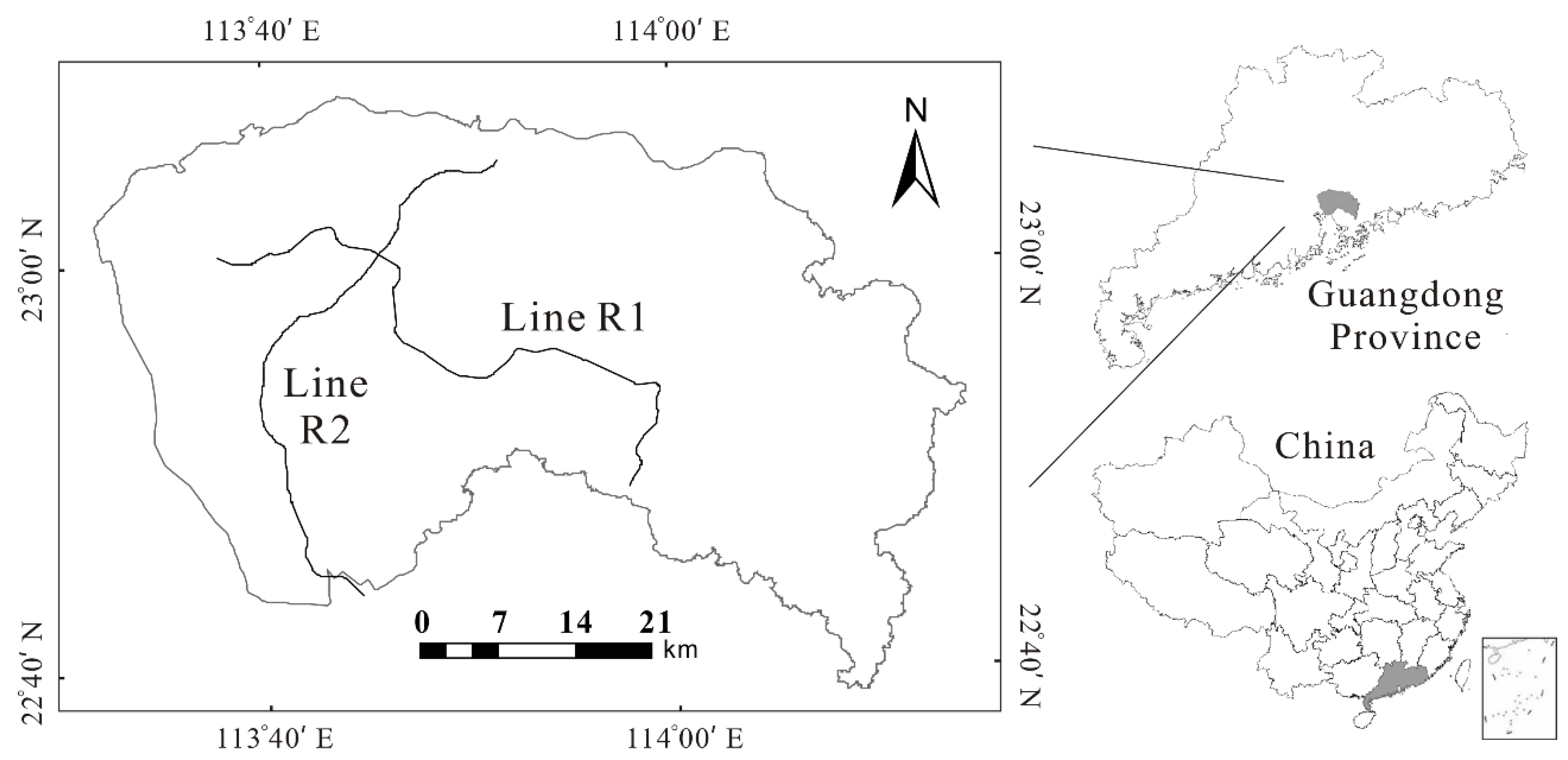
Dongguan is one of the biggest manufacturing bases in China (see Figure 2). This region consists of 4 districts and 28 towns with a total area of about 2465 km2. Although the rapid pace of urbanization in Dongguan has slowed down, it still suffers from a number of “side effects”, such as overpopulation and poor transport accessibility. To alleviate these problems, the People’s Government of Dongguan Municipality decided to build LRTs around 2008. Therefore, it has become an urgent task to assess, simulate, and predict the consequent spatio-temporal dynamics of urban land use.
Land cover is one of the most important data used to demonstrate the effects of land use changes, especially human activities [62]. Production of land use maps can be done by using different methods on satellite images. Some studies have produced land cover maps of the controlled classification technique over Landsat satellite imagery [63,64]. By using land cover maps, the changes in urban development and green areas over time could be evaluated [65]. In this study, we obtained time series of SPOT images in 2006, 2008, 2011, 2013, as well as the blueprints of two LRTs (Line R2 and R1) in Dongguan. Since neither of them has been put into operation when this study began, the three time intervals, 2006–2008, 2008–2011, 2011–2013, respectively correspond to the pre-planning, planning, and construction stages of the LRTs [18,23]. In other words, this study focuses only on the land use changes for these three stages. We visually interpreted all the SPOT images, and then double-checked the results based on Quickbird images and field investigation. The final results include five categories: industrial development, commercial and residential development, rural development, water body, and other land use types. Water bodies are assumed to be constant during the simulation and prediction procedures [66,67,68]. In addition, all the results were resampled to a spatial resolution of 28.5 m for saving computational cost.
3.2. Assessing the Impacts of Line R2 on Its Surrounding Urban Land Use
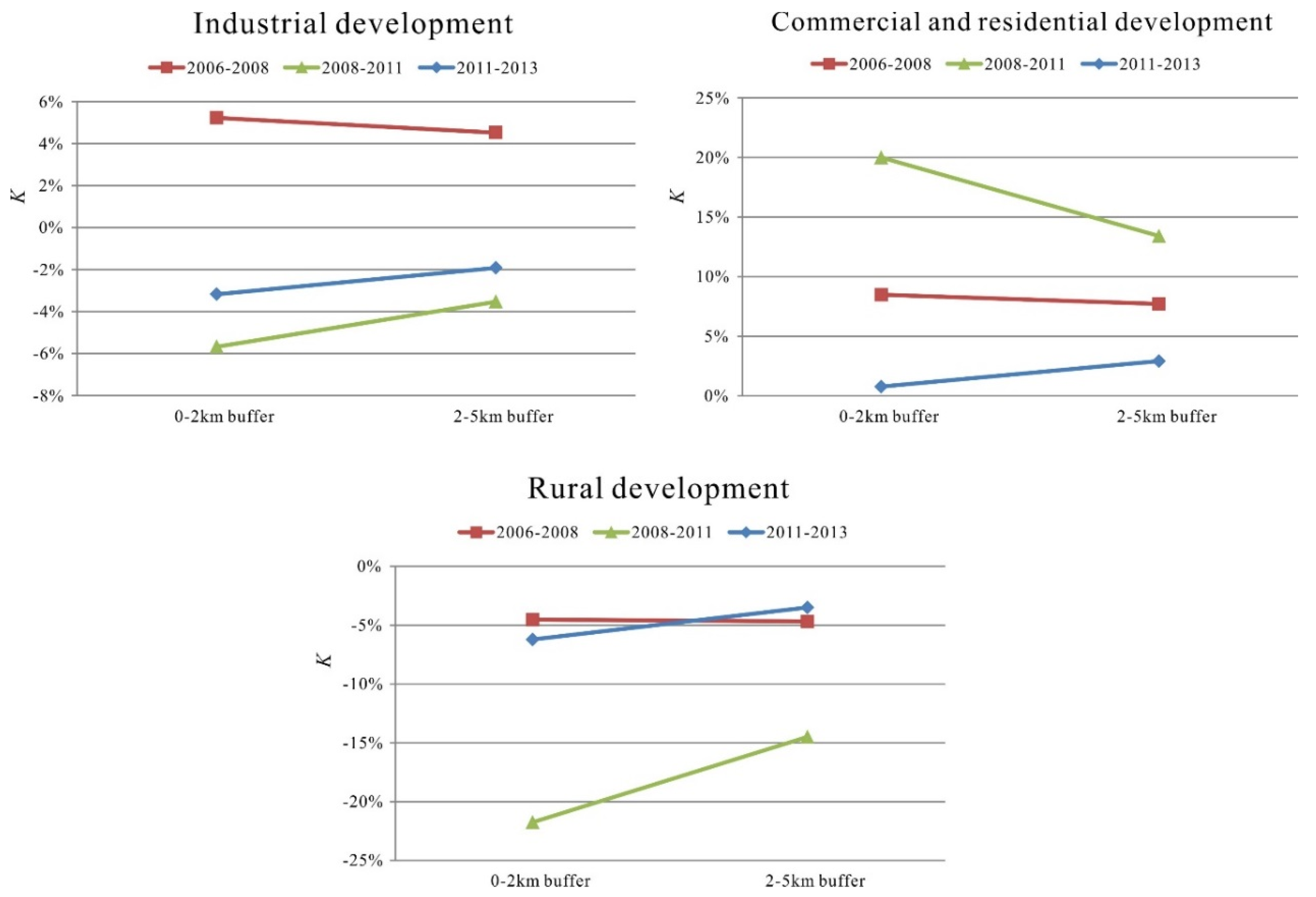
We built a two-sided multi-ring buffer at the interval of 0.5 km for LRT to assess its impacts on surrounding urban land use. The results presented in Figure 3 and Figure 4 indicate that the LRT mainly exerted substantial impacts within the first three or four buffers (i.e., 0–1.5/2 km). The values of “K” (see Equation (1) for the definition) for “0–2 km buffer” and “2–5 km buffer” are quite close at first (during 2006–2008). However, these values become significantly different after the planning of the LRT project. In other words, “K” will become irregular when the buffer size is greater than 1.5/2 km during 2008–2013. Therefore, we just concentrated on the land use changes within the 2 km buffer.
The land use transition matrices at different time intervals are summarized in Table 1. It is found that all three urban land use types changed relatively slightly before the proposition of the line. However, a large amount of industrial development and rural development has been converted to commercial and residential development during the planning stage of R2. Therefore, the area of commercial and residential development exhibited an obvious upward trend. The results indicate that the impacts of LRT investment on urban land use will vary considerably over time. It is unreasonable if we predict potential land use changes associated with a newly planned line simply based on the change trend during the pre-planning stage.
More importantly, we can conclude from Figure 5 that the urban land use changes observed in the whole city were much steadier than the changes within the buffer. In other words, the irregular land use changes within the buffer were mainly driven by the development of LRT since Dongguan was already in a stable period of urbanization. Therefore, the land use change information at the city level cannot be used to predict potential impacts of LRT, either.
3.3. Simulating the Spatial Impacts of Line R2 on Its Surrounding Urban Land Use
The spatial impacts of Line R2 on its surrounding urban land use during the planning stage can be simulated by the well-known ANN-CA. This model was calibrated based on the observed land use maps in 2008 and 2011. The changes in urban development over time can be evaluated by using these land use maps. Since land use change is mainly due to human activities and natural factors, twelve spatial variables (normalized into the range [0, 1]) were adopted in light of previous studies [41,50,69]. A detailed description of them is provided in Table 2. In this study, multinomial logistic regression was employed to analyze the influences and relative importance of these different spatial variables. We adopted the Statistical Package for the Social Sciences (IBM SPSS version 23, Armonk, NY, USA) package for performing the regression. The estimated weights and associated statistics for the variables are displayed in Table S1 (see Supplementary Materials). A positive (or negative) weight means that the variable positively (or negatively) correlates with the land use conversion probability. For example, the conversion probability to CRD will increase as the distance from the cell to the nearest LRT station decreases. By contrast, the conversion probability to RD will decrease in this situation. A higher weight generally implies a stronger influence. Besides, the p-values for these weights are almost all less than 0.05, which indicates that this analysis is statistically significant at the 5% level, and these spatial variables could well explain the urban land use changes in this study. It should also be noted that the following procedures are the same if other variables are used.
Moreover, we analyzed the land use’s proportional changes that would result from a one percent increase in each independent variable mentioned above, while other variables were held constant [70,71]. These results (response elasticities) shown in Table 3 could reflect how land use would respond to the changes in different variables. We found that the “Distance from a cell to the nearest LRT station” is the most influential spatial variable that drives urban land use changes in the study area. The change of this distance could substantially alter the land use proportions. For example, the area of CRD will decrease by about 1.51% when this distance increases by 1% (with response elasticity greater than 1). In addition, the distances to the socioeconomic centers and roadways have negative influences on the area of CRD. The most probable reason for this phenomenon is that those regions closer to the socioeconomic centers and roadways could offer more opportunities for employment and residence. On the contrary, the areas of ID and RD generally increase with the distances to the socioeconomic centers and roadways. The former is more responsive to “Distance to the nearest road”, while the latter is more responsive to “Distance to the nearest town center”. Lastly, we found that “Slope” exerts a negative influence on the areas of ID, CRD, and RD since steeper regions are usually unsuitable for any land use development. Based on the valuable information above, we can build the land use models in the next step.
In this study, the input layer of the network has twelve neurons that represent twelve spatial variables mentioned above. The hidden layer includes eight neurons, while four neurons are used in the output layer to represent four land use types. Each output neuron provides a conversion probability corresponding to one land use type. We used proportional stratified sampling method to separately select 8000 training and 4000 testing samples from the land use maps. Each sample contains a cell’s several attribute values (as listed in Table 2), and its final land use state. The former and the latter will serve as independent and dependent variables, respectively. Therefore, the training objective is to correctly predict the cell’s land use change (i.e., from initial to final land use state) based on the attribute values [50]. 30.21% of the cells changed over the calibration period. Then, the training samples were input into the MATLAB platform for training the ANN-CA, whereas the testing samples were used to check whether the model is overfitted or not. The training parameters in this study were decided through an empirical method, that is, we manually tuned the parameters until acceptable results were obtained. As a result, the learning rate, training epoch, and training goal were set as 0.01, 5000, 0.01, respectively. Finally, the training and testing accuracies are 77.59% and 74.18%.
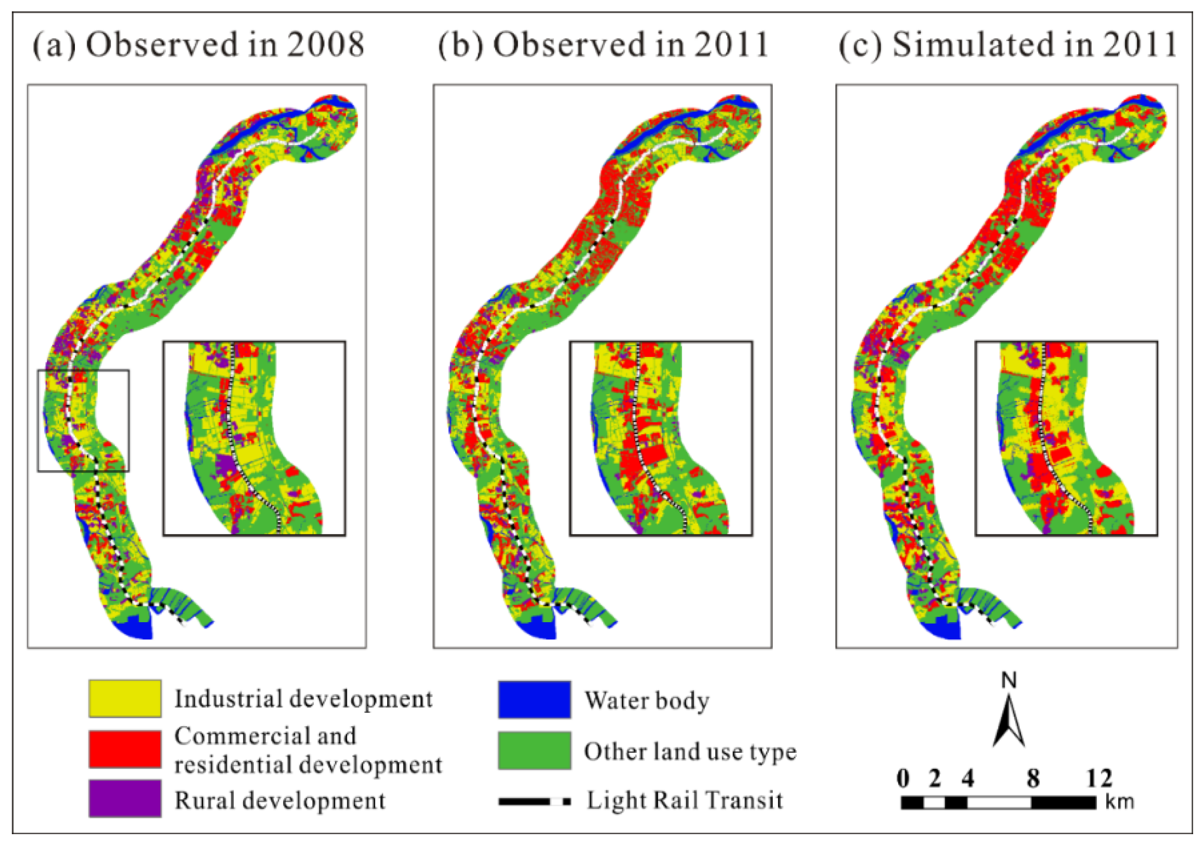
After training the ANN-CA model, we can simulate the spatial dynamics of urban land use around Line R2 from 2008 to 2011. The simulation result was compared with the observed land use map to evaluate the performance of the model. As shown in Figure 6, the spatial patterns of the two maps are quite similar. In addition, confusion matrix and FoM (figure of merit) were employed to further quantify the simulation accuracy. Table 4 and Table 5 present the corresponding confusion matrix and the proportion of different urban land use types within the buffer. Similarly, industrial development and rural development substantially became commercial and residential development in the simulation result. The overall accuracy and FoM value are 72.55% and 31.62% respectively. All these results have demonstrated that the spatial land use changes influenced by LRT development can be well simulated by the calibrated ANN-CA. This model is reliable enough for prediction.
3.4. Predicting the Potential Impacts of Line R1 on Its Surrounding Urban Land Use
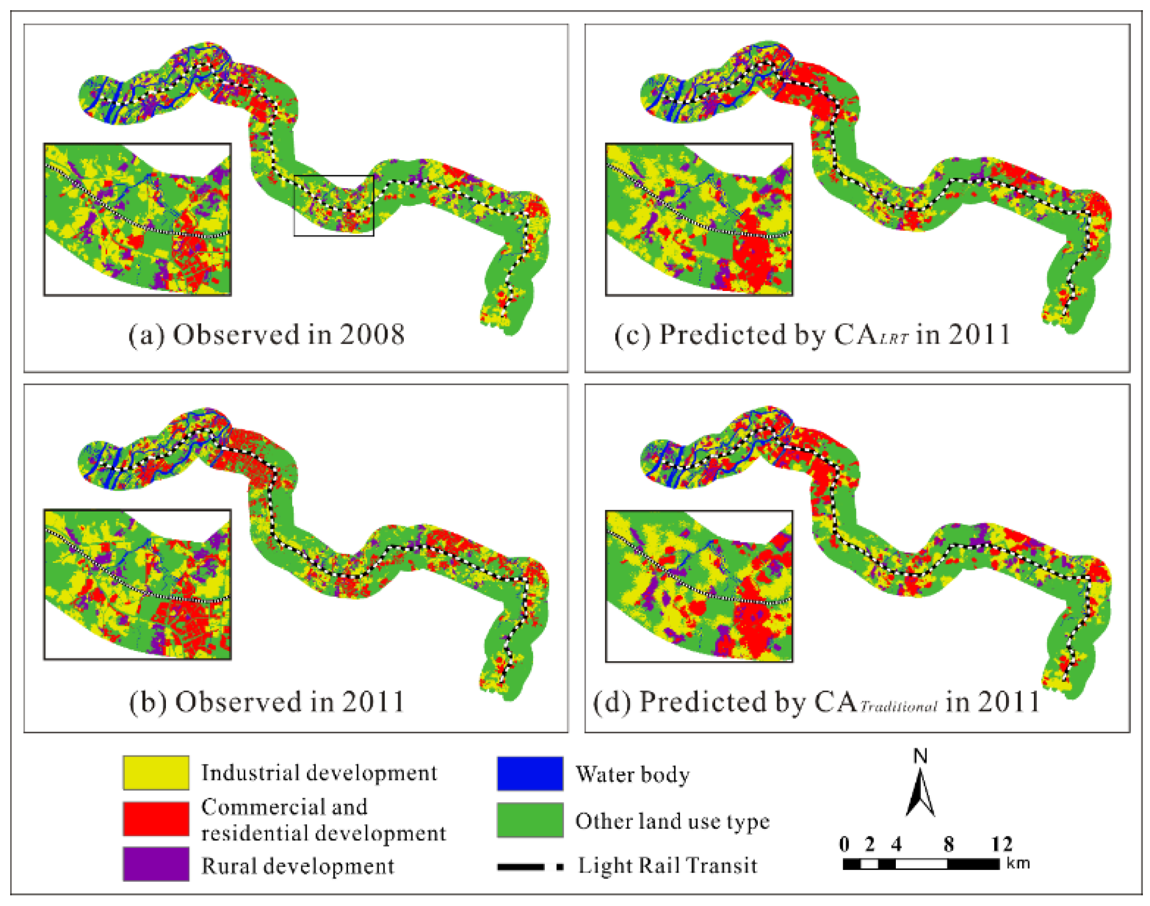
In this study, Line R1 is assumed to be a newly planned line. There are two methods that can be used to predict the potential impacts of R1 on its surrounding urban land use. The first one, which we call “CALRT”, builds on the above calibrated ANN-CA. The other one is a traditional way for LUCC prediction by continuing the preceding change trend of R1 itself (CATraditional hereafter). Specifically, the spatial dynamics of land use from 2008 to 2011 were predicted according to the change information during 2006–2008. The model training procedures are the same as those described in the above subsection. Figure 7 displays a visual comparison between the two prediction results, Table 6 presents the corresponding confusion matrices, and Table 7 shows the proportion of different urban land use types within the buffer.
The cell-based overall accuracies for CALRT and CATraditional are 69.23% and 67.06%, while their FoM are 17.79% and 15.07%. In addition to spatial dynamics, it is found that the quantitative change trend during the planning stage of R1 can also be well predicted by CALRT. With respect to the prediction result by CATraditional, however, the area of industrial development slightly increased, which is contrary to the observed pattern. All these comparisons indicate that our proposed method is more suitable than the traditional method as the former can take the information about the LRT project into consideration.
4. Discussion
The relative responsiveness values of urban land use changes to different independent variables are important in future LRT project identification and land use optimization. Policy-makers need to thoroughly understand how different land uses would change (both spatially and quantitatively) after the planning of LRT projects [72,73]. For example, when a local government decides to construct new LRTs in the near future, our proposed method (CALRT) could be employed to pick out some feasible routes through a pre-assessment of different alternatives. In addition, if policy-makers would like to maintain a sustainable intensity of land use and a balanced distribution of development and population, then the relative responsiveness values should be even more carefully taken into consideration during the planning stage. This valuable information could assist policy-makers in balancing the needs and interests of LRT projects appropriately. For example, LRT projects could be constructed in under-developed or less accessible regions to promote urban and economic development since a shorter distance to LRT stations will generally lead to an increase of the CRD area. By contrast, improving traffic efficiency is the primary purpose of LRT projects in some over-concentrated commercial districts. In this situation, LRT stations could be placed at a certain walking distance from those regions. A collaborative decision-making is still necessary for fashioning the final LRT plans. Compared with the traditional LUCC prediction method (i.e., CATraditional), CALRT may be much more helpful under a changing environment. Besides, urban planners or policy-makers may not only care about a land use model’s cell-based accuracy, but also want to gain more knowledge from previous planning and development experiences through the model. These advantages of CALRT are fundamental to city development since previous studies have indicated that a reasonable transportation network could not only improve transport accessibility, but also contribute to land use reallocation, urban renewal, etc. [73,74]. On the contrary, the investment in LRTs may contribute little to urban development or transport accessibility if the routes are not properly arranged.
In this study, the proposed method was applied to a specific problem and specific region, but it has the potential to be expanded into a broader scale in future studies since these phenomena are not uncommon throughout the world. For example, a city’s potential land use dynamics may be predicted based on the experience from other cities with similar land use change patterns. To do so, we should first analyze the various factors that contribute to land use changes in that case (e.g., how do these factors influence land use changes). If these different regions share similar change patterns, then the proposed method could be applied to the project settings (e.g., model parameter estimation) as well as land use prediction. Although the proposed method shows promise in urban and transportation planning, some aspects still need to be strengthened and explored in the future given the complex relationships between land use and transportation. For example, we should test the effectiveness of our method over different planning stages. Although the two regions in this study share similar land use change pattern, we may need to measure the similarity between different regions/periods in future studies. Besides, Line R1 is assumed to be a newly planned line in this study. We need to test whether our method still works well on truly new lines. In addition, this study only demonstrates that the experiences of LRT impacts can be reused by other lines within the same city (Dongguan). It would also be interesting to see whether those experiences can be generalized for other regions.
5. Conclusions
The emergence of LRTs will inevitably exert great impacts on sustainable urban development, both spatially and quantitatively. It is important to assess, simulate, and particularly predict the potential land use changes if policy-makers decide to build a new line. By analyzing the first LRT of Dongguan (Line R2), this study indicates that such impacts will vary substantially at different stages of the line. For example, the area of commercial and residential development increased during the planning stage, whereas the area of industrial development, and rural development decreased at the same time. By contrast, the urban land use just slightly changed before the proposition of the line. What’s worse, the urban land use changes within the buffer were much more irregular than the changes observed in the whole city. These phenomena pose great problems for land use change prediction since most previous studies assumed that present trends and dynamics of land use change will continue into the future.
To deal with the challenges, our study suggests applying the experiences from Line R2 to the analysis of Line R1 (another LRT in Dongguan) with the help of an ANN-CA model. We first simulated the spatial land use changes within a buffer of R2 from 2008 to 2011 (the planning stage of R2). More importantly, the impacts of R1 on its surrounding urban land use during the same stage were predicted by using two methods. The first one is called CALRT, which takes full advantage of the above land use change information from R2. The other one, CATraditional, is a classical way for LUCC prediction by continuing the preceding change trend of R1 itself. The experiments have demonstrated that our method (CALRT) is more suitable than CATraditional in terms of both visual and quantitative comparisons. For example, the cell-based overall accuracies of the two prediction results are 69.23% and 67.06%, respectively. Compared with CATraditional, the prediction result by CALRT is more close to the observed pattern. The main reason is that the information about the LRT projects can be reasonably considered in CALRT. Our method is expected to provide technical support for sustainable urban and transportation planning.
Supplementary Materials
The following are available online at https://www.mdpi.com/2071-1050/10/4/1293/s1, Table S1: The estimated weights and associated statistics for different spatial variables.
Acknowledgments
This study was supported by the Key National Natural Science Foundation of China (Grant No. 41531176). We thank the academic editor and two anonymous reviewers for their useful comments and suggestions that greatly improved this paper.
Author Contributions
Jinyao Lin conceived and designed the experiments; Tongli Chen and Qiazi Han made substantial contributions to the design, data processing, and analysis; Jinyao Lin wrote the paper; All authors had read and approved the manuscript.
Conflicts of Interest
The authors declare no conflict of interest.
References
- He, C.; Liu, Z.; Tian, J.; Ma, Q. Urban expansion dynamics and natural habitat loss in China: A multiscale landscape perspective. Glob. Chang. Biol. 2014, 20, 2886–2902. [Google Scholar] [CrossRef] [PubMed]
- Liu, X.; Liang, X.; Li, X.; Xu, X.; Ou, J.; Chen, Y.; Li, S.; Wang, S.; Pei, F. A future land use simulation model (FLUS) for simulating multiple land use scenarios by coupling human and natural effects. Landsc. Urban Plan. 2017, 168, 94–116. [Google Scholar] [CrossRef]
- Lin, J.; Liu, X.; Li, K.; Li, X. A maximum entropy method to extract urban land by combining MODIS reflectance, MODIS NDVI, and DMSP-OLS data. Int. J. Remote Sens. 2014, 35, 6708–6727. [Google Scholar] [CrossRef]
- Wang, L.; Li, C.; Ying, Q.; Cheng, X.; Wang, X.; Li, X.; Hu, L.; Liang, L.; Yu, L.; Huang, H.; et al. China’s urban expansion from 1990 to 2010 determined with satellite remote sensing. Chin. Sci. Bull. 2012, 57, 2802–2812. [Google Scholar] [CrossRef]
- Deng, X.; Huang, J.; Rozelle, S.; Uchida, E. Growth, population and industrialization, and urban land expansion of China. J. Urban Econ. 2008, 63, 96–115. [Google Scholar] [CrossRef]
- Zhang, K.H.; Song, S. Rural-urban migration and urbanization in China: Evidence from time-series and cross-section analyses. China Econ. Rev. 2003, 14, 386–400. [Google Scholar] [CrossRef]
- Chan, K.W.; Zhang, L. The Hukou System and Rural-Urban Migration in China: Processes and Changes. China Q. 1999, 160, 818–855. [Google Scholar] [CrossRef]
- National Bureau of Statistics of China. The 2010 Population Census of the People’s Republic of China; China Statistics Press: Beijing, China, 2011.
- Pucher, J.; Peng, Z.; Mittal, N.; Zhu, Y.; Korattyswaroopam, N. Urban transport trends and policies in China and India: Impacts of rapid economic growth. Transp. Rev. 2007, 27, 379–410. [Google Scholar] [CrossRef]
- Shen, Q. Urban transportation in Shanghai, China: Problems and planning implications. Int. J. Urban Reg. Res. 1997, 21, 589–606. [Google Scholar] [CrossRef]
- Cervero, R.; Dai, D. BRT TOD: Leveraging transit oriented development with bus rapid transit investments. Transp. Policy 2014, 36, 127–138. [Google Scholar] [CrossRef]
- Chang, D.T. A new era for public transport development in China. China Environ. Ser. 1999, 3, 22–27. [Google Scholar]
- Wang, X.; Xu, J.; Li, Y. Potential influences of rail transportation construction to land use differentiation in Nanjing. Hum. Geogr. 2005, 20, 112–116. [Google Scholar]
- Zhou, J.; Xu, J. The corridor effects of rail transporation on urban land using. Urban Mass Transit 2002, 5, 77–81. [Google Scholar]
- Li, H.; Peng, J.; Liu, W.; Huang, Z. Stationary charging station design for sustainable urban rail systems: A case study at Zhuzhou Electric Locomotive Co., China. Sustainability 2015, 7, 465–481. [Google Scholar] [CrossRef]
- Pacheco-Raguz, J.F. Assessing the impacts of Light Rail Transit on urban land in Manila. J. Transp. Land Use 2010, 3, 113–138. [Google Scholar] [CrossRef]
- Cervero, R.; Landis, J. Twenty years of the bay area rapid transit system: Land use and development impacts. Transp. Res. Part A Policy Pract. 1997, 31, 309–333. [Google Scholar] [CrossRef]
- Golub, A.; Guhathakurta, S.; Sollapuram, B. Spatial and temporal capitalization effects of light rail in phoenix from conception, planning, and construction to operation. J. Plan. Educ. Res. 2012, 32, 415–429. [Google Scholar] [CrossRef]
- Wegener, M. Land-use transport interaction models. In Handbook of Regional Science; Fischer, M.M., Nijkamp, P., Eds.; Springer: Berlin/Heidelberg, Germany, 2014; pp. 741–758. [Google Scholar]
- Acheampong, R.A.; Silva, E.A. Land use-transport interaction modeling: A review of the literature and future research directions. J. Transp. Land Use 2015, 8, 11–38. [Google Scholar] [CrossRef]
- Jiao, L.; Shen, L.; Shuai, C.; Tan, Y.; He, B. Measuring crowdedness between adjacent stations in an urban metro system: A Chinese case study. Sustainability 2017, 9, 2325. [Google Scholar] [CrossRef]
- Cervero, R. Linking urban transport and land use in developing countries. J. Transp. Land Use 2013, 6, 7–24. [Google Scholar] [CrossRef]
- Yan, S.; Delmelle, E.; Duncan, M. The impact of a new light rail system on single-family property values in Charlotte, North Carolina. J. Transp. Land Use 2012, 5, 60–67. [Google Scholar]
- Bowes, D.R.; Ihlanfeldt, K.R. Identifying the impacts of rail transit stations on residential property values. J. Urban Econ. 2001, 50, 1–25. [Google Scholar] [CrossRef]
- Cervero, R.; Duncan, M. Benefits of proximity to rail on housing markets: Experiences in Santa Clara County. J. Public Transp. 2002, 5, 1–18. [Google Scholar]
- Debrezion, G.; Pels, E.; Rietveld, P. The impact of railway stations on residential and commercial property value: A meta-analysis. J. Real Estate Financ. Econ. 2007, 35, 161–180. [Google Scholar] [CrossRef] [Green Version]
- Mokadi, E.; Mitsova, D.; Wang, X. Projecting the impacts of a proposed streetcar system on the urban core land redevelopment: The case of Cincinnati, Ohio. Cities 2013, 35, 136–146. [Google Scholar] [CrossRef]
- Zhang, X.; Liu, X.; Hang, J.; Yao, D.; Shi, G. Do urban rail transit facilities affect housing prices? Evidence from China. Sustainability 2016, 8, 380. [Google Scholar] [CrossRef]
- Cervero, R. Traffic impacts of variable pricing on the San Francisco-Oakland Bay Bridge, California. Transp. Res. Record J. Transp. Res. Board 2012, 2278, 145–152. [Google Scholar] [CrossRef]
- Fan, Y.; Guthrie, A.; Levinson, D. Impact of light rail implementation on labor market accessibility: A transportation equity perspective. J. Transp. Land Use 2012, 5, 28–39. [Google Scholar] [CrossRef]
- Liggett, R.; Loukaitou-Sideris, A.; Iseki, H. Journeys to crime: Assessing the effects of a light rail line on crime in the neighborhoods. Univ. Calif. Transp. Center 2003, 6, 1–23. [Google Scholar] [CrossRef]
- Nolte, A.; Yacobi, H. Politics, infrastructure and representation: The case of Jerusalem’s light rail. Cities 2015, 43, 28–36. [Google Scholar] [CrossRef]
- Farber, S.; Fu, L. Dynamic public transit accessibility using travel time cubes: Comparing the effects of infrastructure (dis)investments over time. Comput. Environ. Urban Syst. 2017, 62, 30–40. [Google Scholar] [CrossRef]
- Mejia-Dorantes, L.; Paez, A.; Vassallo, J.M. Transportation infrastructure impacts on firm location: The effect of a new metro line in the suburbs of Madrid. J. Transp. Geogr. 2012, 22, 236–250. [Google Scholar] [CrossRef]
- Liu, Y.; Luo, T.; Liu, Z.; Kong, X.; Li, J.; Tan, R. A comparative analysis of urban and rural construction land use change and driving forces: Implications for urban–rural coordination development in Wuhan, Central China. Habitat Int. 2015, 47, 113–125. [Google Scholar] [CrossRef]
- He, J.; Liu, Y.; Yu, Y.; Tang, W.; Xiang, W.; Liu, D. A counterfactual scenario simulation approach for assessing the impact of farmland preservation policies on urban sprawl and food security in a major grain-producing area of China. Appl. Geogr. 2013, 37, 127–138. [Google Scholar] [CrossRef]
- Joshi, H.; Guhathakurta, S.; Konjevod, G.; Crittenden, J.; Li, K. Simulating the effect of light rail on urban growth in phoenix: An application of the UrbanSim modeling environment. J. Urban Technol. 2006, 13, 91–111. [Google Scholar] [CrossRef]
- Basse, R.M. A constrained cellular automata model to simulate the potential effects of high-speed train stations on land-use dynamics in trans-border regions. J. Transp. Geogr. 2013, 32, 23–37. [Google Scholar] [CrossRef]
- Aljoufie, M. Toward integrated land use and transport planning in fast-growing cities: The case of Jeddah, Saudi Arabia. Habitat Int. 2014, 41, 205–215. [Google Scholar] [CrossRef]
- Aljoufie, M.; Zuidgeest, M.; Brussel, M.; Vliet, J.V.; Maarseveen, M.V. A cellular automata-based land use and transport interaction model applied to Jeddah, Saudi Arabia. Landsc. Urban Plan. 2013, 112, 89–99. [Google Scholar] [CrossRef]
- Basse, R.M.; Omrani, H.; Charif, O.; Gerber, P.; Bódis, K. Land use changes modelling using advanced methods: Cellular automata and artificial neural networks. The spatial and explicit representation of land cover dynamics at the cross-border region scale. Appl. Geogr. 2014, 53, 160–171. [Google Scholar] [CrossRef]
- Li, X.; Chen, G.; Liu, X.; Liang, X.; Wang, S.; Chen, Y.; Pei, F.; Xu, X. A new global land-use and land-cover change product at a 1-km resolution for 2010 to 2100 based on human-environment interactions. Ann. Am. Assoc. Geogr. 2017, 107, 1040–1059. [Google Scholar] [CrossRef]
- Aljoufie, M.; Zuidgeest, M.; Brussel, M.; Maarseveen, M.V. Spatial–temporal analysis of urban growth and transportation in Jeddah City, Saudi Arabia. Cities 2013, 31, 57–68. [Google Scholar] [CrossRef]
- Liu, Y.; He, Q.; Tan, R.; Liu, Y.; Yin, C. Modeling different urban growth patterns based on the evolution of urban form: A case study from Huangpi, Central China. Appl. Geogr. 2016, 66, 109–118. [Google Scholar] [CrossRef]
- Pinto, N.; Antunes, A.P.; Roca, J. Applicability and calibration of an irregular cellular automata model for land use change. Comput. Environ. Urban Syst. 2017, 65, 93–102. [Google Scholar] [CrossRef]
- Rienow, A.; Goetzke, R. Supporting sleuth—Enhancing a cellular automaton with support vector machines for urban growth modeling. Comput. Environ. Urban Syst. 2015, 49, 66–81. [Google Scholar] [CrossRef]
- Shafizadeh-Moghadam, H.; Asghari, A.; Tayyebi, A.; Taleai, M. Coupling machine learning, tree-based and statistical models with cellular automata to simulate urban growth. Comput. Environ. Urban Syst. 2017, 64, 297–308. [Google Scholar] [CrossRef]
- Pijanowski, B.C.; Tayyebi, A.; Delavar, M.R.; Yazdanpanah, M.J. Urban expansion simulation using geospatial information system and artificial neural networks. Int. J. Environ. Res. 2010, 3, 493–502. [Google Scholar]
- Tayyebi, A.; Pijanowski, B.C.; Linderman, M.; Gratton, C. Comparing three global parametric and local non-parametric models to simulate land use change in diverse areas of the world. Environ. Model. Softw. 2014, 59, 202–221. [Google Scholar] [CrossRef]
- Li, X.; Yeh, A.G.O. Neural-network-based cellular automata for simulating multiple land use changes using GIS. Int. J. Geogr. Inf. Sci. 2002, 16, 323–343. [Google Scholar] [CrossRef]
- Liu, Y.; Hu, Y.; Long, S.; Liu, L.; Liu, X. Analysis of the Effectiveness of Urban Land-Use-Change Models Based on the Measurement of Spatio-Temporal, Dynamic Urban Growth: A Cellular Automata Case Study. Sustainability 2017, 9, 796. [Google Scholar] [CrossRef]
- Omrani, H.; Tayyebi, A.; Pijanowski, B. Integrating the multi-label land-use concept and cellular automata with the artificial neural network-based land transformation model: An integrated ML-CA-LTM modeling framework. GISci. Remote Sens. 2017, 54, 283–304. [Google Scholar] [CrossRef]
- Pijanowski, B.C.; Tayyebi, A.; Doucette, J.; Pekin, B.K.; Braun, D.; Plourde, J. A big data urban growth simulation at a national scale: Configuring the GIS and neural network based land transformation model to run in a high performance computing (HPC) environment. Environ. Model. Softw. 2014, 51, 250–268. [Google Scholar] [CrossRef]
- Li, S.-M.; Siu, Y.-M. A comparative study of permanent and temporary migration in China: The case of Dongguan and Meizhou, Guangdong Province. Int. J. Popul. Geogr. 1997, 3, 63–82. [Google Scholar] [CrossRef]
- Li, S.; Liu, X.; Li, Z.; Wu, Z.; Yan, Z.; Chen, Y.; Gao, F. Spatial and temporal dynamics of urban expansion along the Guangzhou–Foshan inter-city rail transit corridor, China. Sustainability 2018, 10, 593. [Google Scholar] [CrossRef]
- Wang, X.; Bao, Y. Study on the methods of land use dynamic change research. Prog. Geogr. 1999, 18, 81–87. [Google Scholar]
- Rumelhart, D.E.; Hinton, G.E.; Williams, R.J. Learning representations by back-propagating errors. Nature 1986, 323, 533–536. [Google Scholar] [CrossRef]
- White, R.; Engelen, G. Cellular automata and fractal urban form: A cellular modelling approach to the evolution of urban land-use patterns. Environ. Plan. A 1993, 25, 1175–1199. [Google Scholar] [CrossRef]
- Lin, J.; Li, X. Simulating urban growth in a metropolitan area based on weighted urban flows by using web search engine. Int. J. Geogr. Inf. Sci. 2015, 29, 1721–1736. [Google Scholar] [CrossRef]
- Liu, X.; Li, X.; Shi, X.; Wu, S.; Liu, T. Simulating complex urban development using kernel-based non-linear cellular automata. Ecol. Model. 2008, 211, 169–181. [Google Scholar] [CrossRef]
- Pontius, R.G., Jr.; Boersma, W.; Castella, J.-C.; Clarke, K.; de Nijs, T.; Dietzel, C.; Duan, Z.; Fotsing, E.; Goldstein, N.; Kok, K. Comparing the input, output, and validation maps for several models of land change. Ann. Reg. Sci. 2008, 42, 11–37. [Google Scholar] [CrossRef]
- Naeem, S.; Cao, C.; Fatima, K.; Najmuddin, O.; Acharya, B. Landscape greening policies-based land use/land cover simulation for Beijing and Islamabad—An implication of sustainable urban ecosystems. Sustainability 2018, 10, 1049. [Google Scholar] [CrossRef]
- He, C.; Gao, B.; Huang, Q.; Ma, Q.; Dou, Y. Environmental degradation in the urban areas of China: Evidence from multi-source remote sensing data. Remote Sens. Environ. 2017, 193, 65–75. [Google Scholar] [CrossRef]
- Hassan, M.; Southworth, J. Analyzing land cover change and urban growth trajectories of the mega-urban region of Dhaka using remotely sensed data and an ensemble classifier. Sustainability 2018, 10, 10. [Google Scholar] [CrossRef]
- Lin, J.; Li, X. Conflict resolution in the zoning of eco-protected areas in fast-growing regions based on game theory. J. Environ. Manag. 2016, 170, 177–185. [Google Scholar] [CrossRef] [PubMed]
- Lin, J.; Li, X. Knowledge transfer for large-scale urban growth modeling based on formal concept analysis. Trans. GIS 2016, 20, 684–700. [Google Scholar] [CrossRef]
- Liu, X.; Li, X.; Liu, L.; He, J.; Ai, B. A bottom-up approach to discover transition rules of cellular automata using ant intelligence. Int. J. Geogr. Inf. Sci. 2008, 22, 1247–1269. [Google Scholar] [CrossRef]
- Chen, Y.; Li, X.; Liu, X.; Ai, B.; Li, S. Capturing the varying effects of driving forces over time for the simulation of urban growth by using survival analysis and cellular automata. Landsc. Urban Plan. 2016, 152, 59–71. [Google Scholar] [CrossRef]
- Liu, X.; Ma, L.; Li, X.; Ai, B.; Li, S.; He, Z. Simulating urban growth by integrating landscape expansion index (LEI) and cellular automata. Int. J. Geogr. Inf. Sci. 2014, 28, 148–163. [Google Scholar] [CrossRef]
- Hardie, I.; Parks, P.; Gottleib, P.; Wear, D. Responsiveness of rural and urban land uses to land rent determinants in the U.S. South. Land Econ. 2000, 76, 659–673. [Google Scholar] [CrossRef]
- Pryce, G. Construction elasticities and land availability: A two-stage least-squares model of housing supply using the variable elasticity approach. Urban Stud. 1999, 36, 2283–2304. [Google Scholar] [CrossRef]
- Ustaoglu, E.; Williams, B.; Murphy, E. Integrating CBA and land-use development scenarios: Evaluation of planned rail investments in the greater Dublin Area, Ireland. Case Stud. Transp. Policy 2016, 4, 104–121. [Google Scholar] [CrossRef]
- Ratner, K.A.; Goetz, A.R. The reshaping of land use and urban form in Denver through transit-oriented development. Cities 2013, 30, 31–46. [Google Scholar] [CrossRef]
- Priemus, H.; Konings, R. Light rail in urban regions: What Dutch policymakers could learn from experiences in France, Germany and Japan. J. Transp. Geogr. 2001, 9, 187–198. [Google Scholar] [CrossRef]
Figure 1.
Flowchart for predicting the spatial impacts of Light Rail Transits on urban land use.

Figure 2.
Location of the study area.

Figure 3.
Land use change rate within different buffers over different periods.
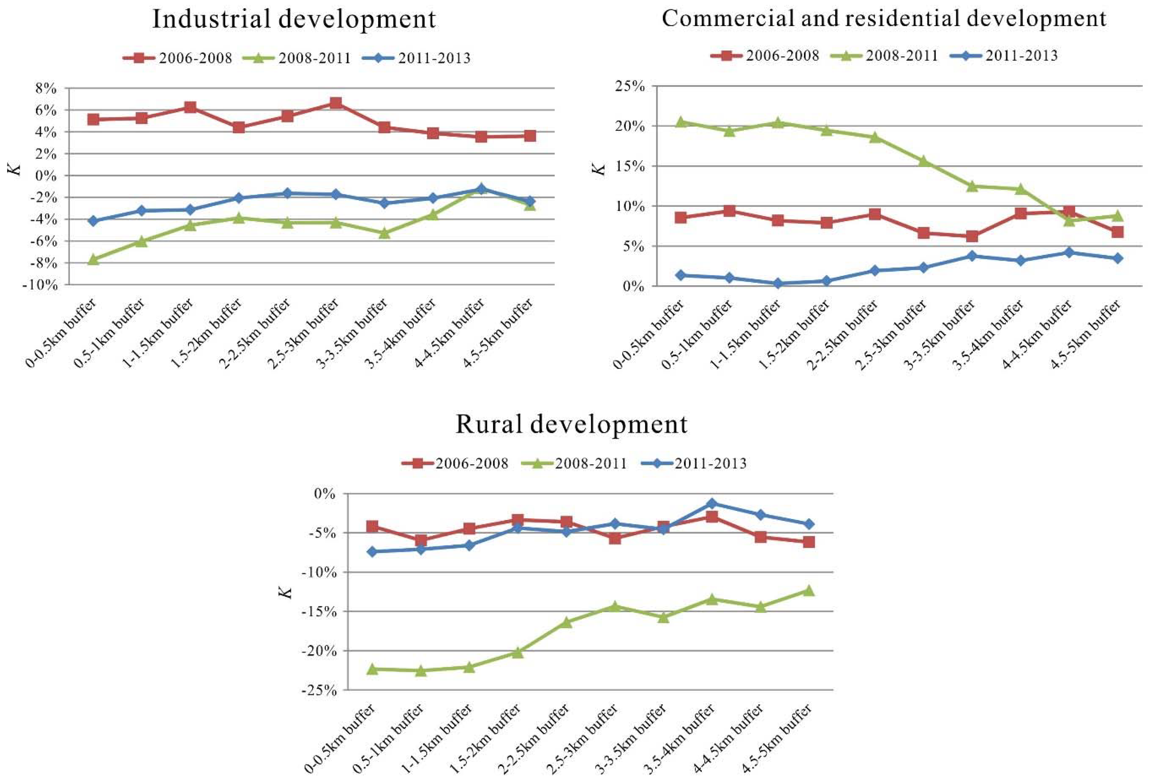
Figure 4.
Comparison of land use change rate between “0–2 km buffer” and “2–5 km buffer”.

Figure 5.
Comparison of urban land use change pattern between “2 km buffer of Line R2” and “Dongguan”.
Figure 5.
Comparison of urban land use change pattern between “2 km buffer of Line R2” and “Dongguan”.
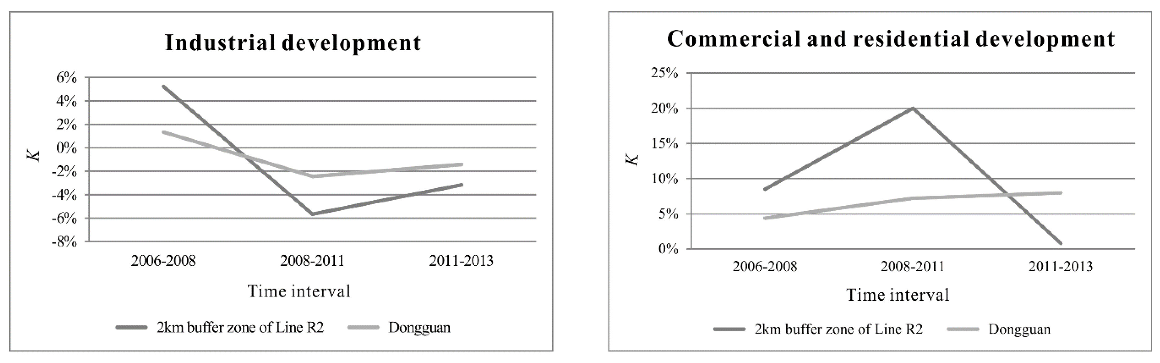
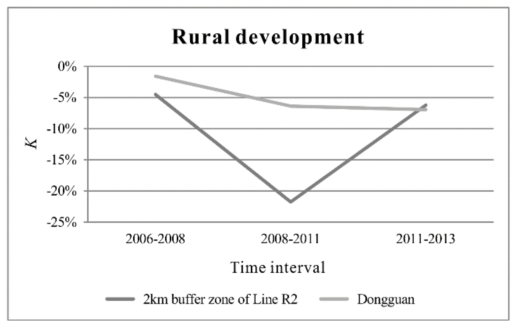
Figure 6.
Simulation of urban land use changes within a 2 km buffer of Line R2: (a) observed in 2008; (b) observed in 2011; and (c) simulated in 2011.
Figure 6.
Simulation of urban land use changes within a 2 km buffer of Line R2: (a) observed in 2008; (b) observed in 2011; and (c) simulated in 2011.

Figure 7.
Prediction of urban land use changes within a 2 km buffer of Line R1: (a) observed in 2008; (b) observed in 2011; (c) predicted by CALRT in 2011; and (d) predicted by CATraditional in 2011.
Figure 7.
Prediction of urban land use changes within a 2 km buffer of Line R1: (a) observed in 2008; (b) observed in 2011; (c) predicted by CALRT in 2011; and (d) predicted by CATraditional in 2011.


Table 1.
Land use transition matrices within a 2 km buffer of Line R2 (in km2).
| Land Use Type | 2008 (Observed) | |||||
|---|---|---|---|---|---|---|
| ID | CRD | RD | OLU | Total | ||
| 2006 (Observed) | ID | 46.91 | 0.27 | 0.11 | 0.43 | 47.72 |
| CRD | 0.42 | 27.58 | 0.10 | 0.57 | 28.66 | |
| RD | 0.34 | 1.89 | 19.47 | 0.22 | 21.91 | |
| OLU | 5.04 | 3.79 | 0.25 | 96.97 | 106.06 | |
| Total | 52.70 | 33.52 | 19.93 | 98.19 | 204.34 | |
| 2011 (Observed) | ||||||
| 2008 (Observed) | ID | 32.67 | 10.99 | 0.39 | 8.65 | 52.70 |
| CRD | 1.83 | 23.42 | 0.58 | 7.70 | 33.52 | |
| RD | 0.85 | 11.92 | 4.98 | 2.18 | 19.93 | |
| OLU | 8.38 | 7.32 | 0.95 | 81.54 | 98.19 | |
| Total | 43.73 | 53.64 | 6.90 | 100.07 | 204.34 | |
| 2013 (Observed) | ||||||
| 2011 (Observed) | ID | 38.68 | 0.68 | 0.17 | 4.20 | 43.73 |
| CRD | 0.21 | 49.98 | 0.08 | 3.37 | 53.64 | |
| RD | 0.10 | 0.56 | 5.62 | 0.62 | 6.90 | |
| OLU | 1.96 | 3.27 | 0.17 | 94.67 | 100.07 | |
| Total | 40.95 | 54.48 | 6.04 | 102.86 | 204.34 | |
Notes (the same below): ID denotes industrial development, CRD denotes commercial and residential development, RD denotes rural development, and OLU denotes other land use types.
Table 2.
Spatial variables used for simulating and predicting urban land use changes.
| Spatial Variable | Acquisition Method |
|---|---|
| Distance from a cell to the city center | Euclidean Distance function in ArcGIS |
| Distance from a cell to the nearest town center | |
| Distance from a cell to the nearest LRT station | |
| Distance from a cell to the nearest highway | |
| Distance from a cell to the nearest railway | |
| Distance from a cell to the nearest road | |
| Area of industrial development within a cell’s 3 × 3 Moore neighborhood | Focal Statistics function in ArcGIS |
| Area of commercial and residential development within a cell’s 3 × 3 Moore neighborhood | |
| Area of rural development within a cell’s 3 × 3 Moore neighborhood | |
| Area of other land use types within a cell’s 3 × 3 Moore neighborhood | |
| Current land use type | Remote sensing image classification |
| Slope | Derived from DEM |
Table 3.
Relative responsiveness of land use changes to different spatial variables.
| City Center | Town Center | LRT Station | Highway | Railway | Road | Slope | |
|---|---|---|---|---|---|---|---|
| ID | 0.40% | 0.17% | 0.42% | 0.19% | 0.38% | −1.15% | −0.58% |
| CRD | −0.69% | −1.28% | −1.51% | −0.35% | −0.20% | −0.61% | −0.33% |
| RD | 0.64% | 1.20% | 1.28% | −0.32% | 0.72% | 0.56% | −0.24% |
| OLU | 0.11% | 0.51% | 0.50% | 0.16% | −0.18% | 0.90% | 0.54% |
Table 4.
Confusion matrix for simulating urban land use changes within a 2 km buffer of Line R2 (in km2).
Table 4.
Confusion matrix for simulating urban land use changes within a 2 km buffer of Line R2 (in km2).
| Land Use Type | 2011 (Simulated) | ||||||
|---|---|---|---|---|---|---|---|
| ID | CRD | RD | OLU | Total | Omission Error | ||
| 2011 (Observed) | ID | 31.81 | 3.98 | 0.96 | 6.97 | 43.73 | 27.26% |
| CRD | 5.61 | 36.73 | 4.64 | 6.66 | 53.64 | 31.52% | |
| RD | 0.48 | 1.22 | 4.25 | 0.95 | 6.90 | 38.41% | |
| OLU | 10.08 | 11.88 | 2.64 | 75.45 | 100.07 | 24.60% | |
| Total | 47.98 | 53.82 | 12.50 | 90.04 | 204.34 | ||
| Commission Error | 33.70% | 31.75% | 66.00% | 16.20% | |||
Table 5.
Proportion of different urban land use types within a 2 km buffer of Line R2 in 2008 and 2011.
Table 5.
Proportion of different urban land use types within a 2 km buffer of Line R2 in 2008 and 2011.
| Land Use Type | 2008 (Observed) | 2011 (Observed) | 2011 (Simulated) | |||
|---|---|---|---|---|---|---|
| Area/km2 | Percent/% | Area/km2 | Percent/% | Area/km2 | Percent/% | |
| Industrial development | 52.70 | 25.79 | 43.73 | 21.40 | 47.98 | 23.48 |
| Commercial and residential development | 33.52 | 16.41 | 53.64 | 26.25 | 53.82 | 26.34 |
| Rural development | 19.93 | 9.75 | 6.90 | 3.38 | 12.50 | 6.12 |
| Other land use | 98.19 | 48.05 | 100.07 | 48.97 | 90.04 | 44.06 |
Table 6.
Confusion matrices for predicting urban land use changes within a 2 km buffer of Line R1 (in km2).
Table 6.
Confusion matrices for predicting urban land use changes within a 2 km buffer of Line R1 (in km2).
| Land Use Type | 2011 (Observed) | ||||||
|---|---|---|---|---|---|---|---|
| ID | CRD | RD | OLU | Total | Commission Error | ||
| 2011 (Predicted by CALRT) | ID | 28.52 | 4.04 | 0.84 | 16.54 | 49.93 | 42.88% |
| CRD | 4.97 | 26.07 | 1.10 | 13.47 | 45.61 | 42.84% | |
| RD | 0.92 | 4.77 | 3.72 | 3.03 | 12.44 | 70.10% | |
| OLU | 12.30 | 10.21 | 2.47 | 109.63 | 134.61 | 18.56% | |
| Total | 46.71 | 45.09 | 8.13 | 142.67 | 242.60 | ||
| Omission Error | 38.94% | 42.18% | 54.24% | 23.16% | |||
| 2011 (Predicted by CATraditional) | ID | 28.23 | 9.80 | 0.77 | 18.56 | 57.37 | 50.79% |
| CRD | 5.72 | 24.86 | 2.62 | 12.12 | 45.32 | 45.15% | |
| RD | 1.54 | 4.17 | 3.27 | 5.66 | 14.63 | 77.65% | |
| OLU | 11.21 | 6.26 | 1.47 | 106.34 | 125.28 | 15.12% | |
| Total | 46.71 | 45.09 | 8.13 | 142.67 | 242.60 | ||
| Omission Error | 39.56% | 44.87% | 59.78% | 25.46% | |||
Table 7.
Proportion of different urban land use types within a 2 km buffer of Line R1 in 2008 and 2011.
Table 7.
Proportion of different urban land use types within a 2 km buffer of Line R1 in 2008 and 2011.
| Land Use Type | 2008 (Observed) | 2011 (Observed) | 2011 (Predicted by CALRT) | 2011 (Predicted by CATraditional) | ||||
|---|---|---|---|---|---|---|---|---|
| Area/km2 | Percent/% | Area/km2 | Percent/% | Area/km2 | Percent/% | Area/km2 | Percent/% | |
| Industrial development | 55.52 | 22.89 | 46.71 | 19.25 | 49.93 | 20.58 | 57.37 | 23.65 |
| Commercial and residential development | 25.21 | 10.39 | 45.09 | 18.59 | 45.61 | 18.80 | 45.32 | 18.68 |
| Rural development | 18.98 | 7.83 | 8.13 | 3.35 | 12.44 | 5.13 | 14.63 | 6.03 |
| Other land use | 142.88 | 58.89 | 142.67 | 58.81 | 134.61 | 55.49 | 125.28 | 51.64 |
© 2018 by the authors. Licensee MDPI, Basel, Switzerland. This article is an open access article distributed under the terms and conditions of the Creative Commons Attribution (CC BY) license (http://creativecommons.org/licenses/by/4.0/).
Share and Cite
MDPI and ACS Style
Lin, J.; Chen, T.; Han, Q. Simulating and Predicting the Impacts of Light Rail Transit Systems on Urban Land Use by Using Cellular Automata: A Case Study of Dongguan, China. Sustainability 2018, 10, 1293. https://doi.org/10.3390/su10041293
AMA Style
Lin J, Chen T, Han Q. Simulating and Predicting the Impacts of Light Rail Transit Systems on Urban Land Use by Using Cellular Automata: A Case Study of Dongguan, China. Sustainability. 2018; 10(4):1293. https://doi.org/10.3390/su10041293
Chicago/Turabian StyleLin, Jinyao, Tongli Chen, and Qiazi Han. 2018. "Simulating and Predicting the Impacts of Light Rail Transit Systems on Urban Land Use by Using Cellular Automata: A Case Study of Dongguan, China" Sustainability 10, no. 4: 1293. https://doi.org/10.3390/su10041293
Note that from the first issue of 2016, this journal uses article numbers instead of page numbers. See further details here.