Article

Assessment of the Ecosystem Service Function of Sandy Lands at Different Times Following Aerial Seeding of an Endemic Species

1
School of Ecology and Environment, Inner Mongolia University, Hohhot 010021, China
2
Inner Mongolia Academy of Forestry Sciences, Hohhot 010010, China
3
College of Grassland, Resources and Environment, Inner Mongolia Agriculture University, Hohhot 010020, China
*
Authors to whom correspondence should be addressed.
Sustainability 2018, 10(4), 902; https://doi.org/10.3390/su10040902
Submission received: 2 February 2018 / Revised: 4 March 2018 / Accepted: 19 March 2018 / Published: 21 March 2018

Abstract

:
Desertification is a global and pressing environmental problem in the course of environmental changes, and considerable efforts have been made to restore these degraded ecosystems. Aerial seeding has been widely used to accelerate ecological restoration around the world. However, few efforts have been made to assess the ecosystem service function after aerial seeding has occurred. In this study, we analyzed variations in the ecosystem service function after varying periods of elapsed time after aerial seeding of Hedysarum laeve Maxim. (14a, 30a and 38a) in the Mu Us Sandy Land, China. We also assessed the carbon sequestration ability, biodiversity, soil properties, wind-break and sand-fixation ability on a typical windward slope. We found that the overall assessment value of ecosystem services had generally increased with the elapsed time after aerial seeding. Additionally, the assessment values increased as the slope position moved downwards. Moreover, we observed a gradual replacement of H. laeve by Artemisia ordosica Krasch and grass species with the increase in elapsed years after aerial seeding, indicating a positive succession towards locally native vegetation. Compared with the local natural vegetation, our results suggest that the practice of aerial seeding stimulated vegetation restoration without the need for follow-up field interventions, and the practice of aerial seeding might fit more ecosystems with similar vegetation degradation problems.

1. Introduction

Desertification is a global environmental problem, and the expansion of desertified land has threatened the sustainable development of human society [1]. It is generally agreed that restoration of the degraded vegetation can efficiently curb desertification. Restoration of the degraded vegetation will improve the ecosystem services [2,3,4]. Natural vegetation recovery can form a more rational and stable structure [5] and is a simple way of restoring vegetation [6]. However, in harsh environments with very few seeds, such as sandy areas, natural regeneration and subsequent forest succession may take much longer time [7,8]. To overcome this issue, aerial seeding is commonly applied to promote vegetation recovery and thus, shorten the time required for ecosystem restoration. Aerial seeding uses the plane as platform, broadcasts the tree (grass) seed on the proper ground to make the seeds germinate, with the help of natural rainfall and optimum temperature, due to the characteristics of forest’s natural renewal ability, and with such methods the forest resources could sequentially expand and the forest vegetation increase. Aerial seeding has been widely used around the world [9,10,11,12,13]. Nevertheless, aerial seeding as a means of vegetation recovery, and its effectiveness on the restoration of ecosystem service function, has been rarely examined [9].
Some recovery plans illustrate the benefits of implementing biodiversity and providing ecosystem services in practice [14], while other examples indicate that restoration will not automatically enhance both biodiversity and services [15,16]. Both positive and negative outcomes of the practice of vegetation restoration by aerial seeding were also reported. For instance, Greipsson et al. [10] found aerial seeding of Festuca rubra L. in Iceland did not create a lasting coverage and facilitate rapid succession, F. rubra disappeared in 10 years after aerial seeding. At the same time, he also found that, with the increasing years after aerial seeding, mosses, plant litter and native forbs started to increase. These studies demonstrate that vegetation restoration is a complicated process resulting from the behavior of component populations and species [17]. Therefore, a systematic assessment of the ecosystem services after the seeding is highly necessary. Studying the spatiotemporal changes of ecosystem service function of a particular vegetation type will help guide the relative authorizes to make their restoration effort in a more efficient way at landscape to regional scale.
Here, we synthesized a unique dataset composed of census data of plant communities and soil samples from landscapes after varying periods of elapsed time after aerial seeding (14a, 30a and 38a), control and the local natural vegetation in the Mu Us Sandy Land. Mu Us Sandy Land, one of the four main sandy lands in China, is among the areas undergoing current desertification [18]. To effectively curb desertification and improve the local ecological and living conditions, aerial seeding has become the primary means of vegetation restoration used to combat desertification and is prominently used in this region. In this region, the seeding species is Hedysarum leave Maxim., which is an endemic shrub species, accounting for approximately one-quarter of the total area of artificial shrubbery in this region [19]. Till now, there is a nearly 40 year history of aerial seeding in this region (since 1978a), which is an ideal research area. We assessed the spatio-temporal changes of ecosystem service function of all sample plots by using the analytic hierarchy process (AHP), including carbon sequestration ability, biodiversity, soil properties, wind-break and sand-fixation ability on the typical windward slope. We wanted to test the hypotheses that aerial seeding of H. laeve would stimulate the succession of degraded ecosystem towards local natural vegetation and the ecosystem service will be restored. Given that the ecosystem services are supplied at various spatial scales, which are also critical in ecosystem management [20]. We further analyzed the ecosystem services by slope positions to test the hypothesis that the restoration performance would be varying between slope positions due to the microhabitat differences.

2. Materials and Methods
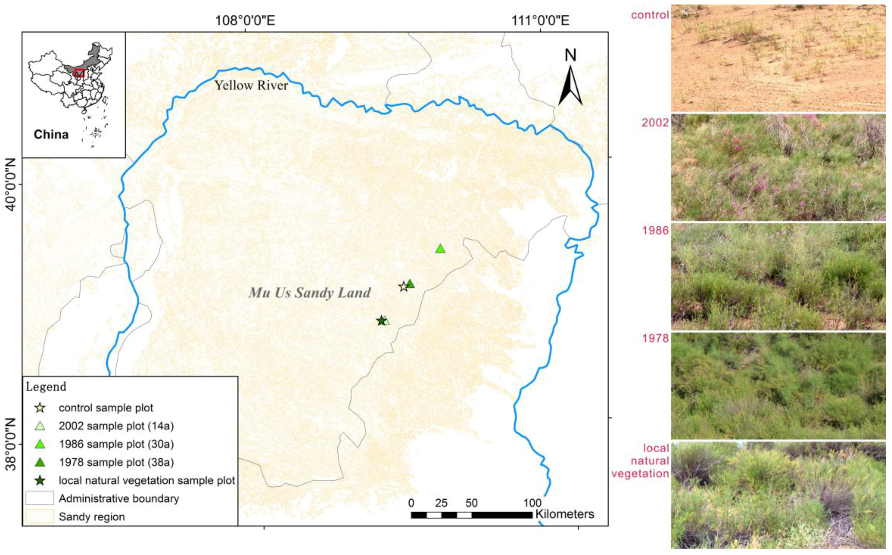
2.1. Study Area

The study was conducted in the hinterland of the Mu Us Sandy Land (37°27′30′′ N–39°22′30′′ N, 107°20′ E–111°30′ E), in Wushen County and Yinjinhuoluo County, Inner Mongolia, China. The altitude ranges from 1200 m to 1600 m in the study area. The annual average temperature is 6.0–8.5 °C, annual rainfall is 250–440 mm, and most of it falls in August. The zonal vegetation in the region is a part of the Eurasian steppe; because of the sand matrix and special climate conditions, semi-fixed and fixed sand dunes are widely distributed. Common shrub species in the research region include Artemisia ordosica Krasch, Salix cheilophila Schneid., H. laeve, Caragana intermedia Kuang et H. C. Fu and Sabina vulgaris Ant. [21].

2.2. Sample Plot Setup and Data Collection

The samples investigated included aerial seeding in 2002, 1986 and 1978, control and local natural vegetation, and all data on community characteristics and soil samples were collected in August and September 2015, that is to say, aerial seeding in 2002, 1986 and 1978 represented 14a, 30a and 38a after aerial seeding, respectively. Because the windward slope has a shallower slope and well-preserved vegetation, the survey was carried out on the windward slope. The sample plots are shown in Table 1, and the geographic location and photos of the sample plots are shown in Figure 1.

2.2.1. Plant Community Investigation

The data were collected along the slope, from the bottom to the middle slope to the top, with four replicates for each slope position. Specifically, a quadrat of 5 m × 5 m was used for shrub plots. Within each quadrat, we recorded the species name, the crown width and height of each individual, the numbers of dead and living branches, the ground diameter of each individual and the aboveground biomass of each individual (i.e., the weight of the plant after being dried at 75 °C). A herb quadrat of 1 m × 1 m was used for each herb quadrat. The species name, the coverage height and the number of each species were recorded, and the aboveground biomass of each species was determined after being dried at 65 °C. The habitat characteristics, such as latitude and longitude, altitude, and soil type, were also recorded.

2.2.2. Soil Sampling and Laboratory Analyses

The soil was sampled in every shrub quadrat at depths of 0–20 cm and 20–40 cm. In the laboratory, soil samples were air-dried. After drying, coarse gravel, rubble, and biotic residuals were carefully picked out and discarded. Soil organic matter (SOM) was analyzed using the potassium permanganate volume method, total nitrogen (TN) was analyzed with the Kjeldahl procedure, soil available phosphorus (SAP) was measured by the 0.5 M NaHCO3 method, and soil available potassium (SAK) was tested by flame photometry (ISSCAS 1978) [22].

2.2.3. Long-Term Monitoring of Soil Moisture

A time-domain reflectometry (TDR) measurement tube (2 m) was buried in every shrub quadrat in May 2015. Then, we measured soil moistures at depth layers of 0–20 cm, 20–40 cm, 40–60 cm, 60–80 cm, 80–100 cm, 100–120 cm, 120–140 cm, 140–160 cm and 160–180 cm separately, using the TRIME-PICO-BT (It’s a soil moisture collection module.) portable soil water quick-test device, in August and November 2015, and April, June, September and November 2016. Soil water data were measured using the PICO-BT portable soil water quick-test device at each soil depth with three replicates.

2.2.4. Long-Term Monitoring of Wind Erosion

The wind erosion spile was buried in May 2015 in every shrub quadrat. We measured wind erosion spile height in November 2015 and November 2016 and calculated the differences to represent the wind erosion conditions.

2.3. Assessment Method

In this study, considering that the basic goal of sand vegetation restoration is the improvement of its ecosystem service function, so we used analytic hierarchy process (AHP) to build ecosystem service function assessment system referring to “Specifications for assessment of forest ecosystem services in China” [23], which included a total target layer (A layer), five criteria layers (B layer), and 10 index layers (C layer) (Table 2).
We used the bar graph to analyze the difference of each index, and we also determined the combined weight of each index for the overall assessment [24,25]. Firstly, we conducted the consultation from relevant experts (In this study, 30 questionnaires were issued. The research area of consulting experts included soil erosion and desertification control, ecology, forest cultivation and management, and their professional title included professor, associate professor and assistant researcher, and so on. Specific questionnaire items included the importance of the five criteria layers, and the importance of the 10 index layers in their respective criteria layer, “1” represented the most important, “2” represented secondarily important, and so on.), used 1~9 scaling method as importance quantitative judgment between assessment factors, and formed a judgment matrix. Secondly, according to the judgment matrix, the relative weight vector of each factors at the same level was calculated by using the root method, and the relative importance weight vector (combined weight) to the criteria layers of all indices was calculated too (Table 2). Finally, we carried out the consistency check of judgment matrix, in other words, we calculated consistency index (CI) and found the appropriate mean random index (RI), and then obtained consistency ratio (CR) = CI/RI. When CR < 0.1, we generally consider the judgment matrix to be of satisfactory consistency, while when CR ≥ 0.1, we need to adjust the judgment matrix until we are satisfied. Under the general situation, the first order and second order matrix is always consistent and CR equals to 0. In this study, for the criterion layer, we found CI = 0, RI = 1.12, and CR = 0 < 0.1, so the judgment matrix had satisfactory consistency.
In this study, as illustrated in Table 2, apparently wind-break and sand-fixation combination weight is the largest (0.42), biodiversity is second (0.25), that is to say, consulting experts believed that windbreak and sand-fixation efficiency and biodiversity are the most important functions in sandy land ecosystem service function assessment system.

2.4. Data Analysis

2.4.1. Data Preparation

According to Table 2, we calculated the aboveground biomass per unit area of shrub (ABS) and herb (ABH) using Equations (1) and (2), respectively, and calculated importance values (IVs) and the various relevant diversity indices, including richness index (R), Simpson index (D), and Shannon–Wiener index (H), using Equations (3)–(6), respectively.
A B S = ( b i o m a s s s ) / 25
A B H = b i o m a s s h
I V s = ( R e l a t i v e   d e n s i t y + R e l a t i v e   f r e q u e n c y + R e l a t i v e   c o v e r a g e ) / 3
R = S
D = 1 P i 2
H = P i lg P i
In Equation (1), b i o m a s s s (g·m−2) is aboveground biomass of each shrub individual, s is the number of individuals of the shrub, and in Equation (2), b i o m a s s h (g·m−2) is the aboveground biomass of each herb individual, h is the number of species of the herb. The relative density of this species is equal to the abundance of this species divided by the total abundance of all the species, the relative frequency and relative coverage of this species were calculated in the same way, IVs have a range 0–1. S is the number of species within 1 m2, P i = n i / N , n i is the number of individuals of each species, i is the species i , and N is the total individual number of all species.

2.4.2. Un-Dimensioned of Data and Calculated the Final Assessment Value

Because all the data had different dimensions, the dimensionless method was applied to all data before assessment. Positive and negative indices were calculated using Equations (7) and (8), respectively. The final assessment value ( Y k ) was obtained using Equation (9).
X k j = X k j / X max × 100 ( X k j X max )
X k j = X min / X k j × 100 ( X k j X min )
Y k = j = 1 m w j X k j
Here, k is the sample plot k ; j is the ecosystem services function index j ; X is the values of the 10 indices in any sample plot; X k j is a measuring value of the ecosystem services function index j in the sample plot k ; X max is the maximum value of an ecosystem services function index; X min is the minimum value of an ecosystem services function index; X k j is a dimensionless value of the ecosystem services function index j in the sample plot k ; Y k is the final assessment value of the sample plot k ; w j is the combined weight of the ecosystem services function index j (Table 2); and m is the number of the ecosystem services function index (equal to 10).

2.4.3. Statistical Analysis

The assessment indices were analyzed in Microsoft Excel 2007 (Microsoft Corporation, Redmond, WA, USA). And to assess how service indices changed with the increase in years since aerial seeding, we conducted one-way ANOVA analysis, used least-significant-difference (LSD) tests to determine which values had significant differences, and believed that the value was significantly different at P < 0.05. We also calculated Pearson correlation coefficients to test for relationships between the ecosystem function service indices. All statistical analysis was conducted using SPSS 19.0 (SPSS Inc., Chicago, IL, USA).

3. Results

3.1. Community Species Importance Values Change

With the increase in aerial seeding duration, the importance value of H. laeve decreased from 0.9502 (14a) to 0.6255 (30a), and finally, to 0.4994 (38a), while the importance value of A. ordosica increased from 0.0498 (14a) to 0.3745 (30a), and finally, to 0.5006 (38a) (Table 3), succession after aerial seeding was moving in the direction towards native vegetation (A. ordosica community, Table 3). Contrasted with control, vegetation restoration was evident, and control had not even shrub. Moreover, with the increase in aerial seeding duration, the grass species that appeared in the herb layer, such as Poa sphondylodes (30a) and Leymus chinensis (38a), were signs of a more stable community, resembling to the local natural vegetation.

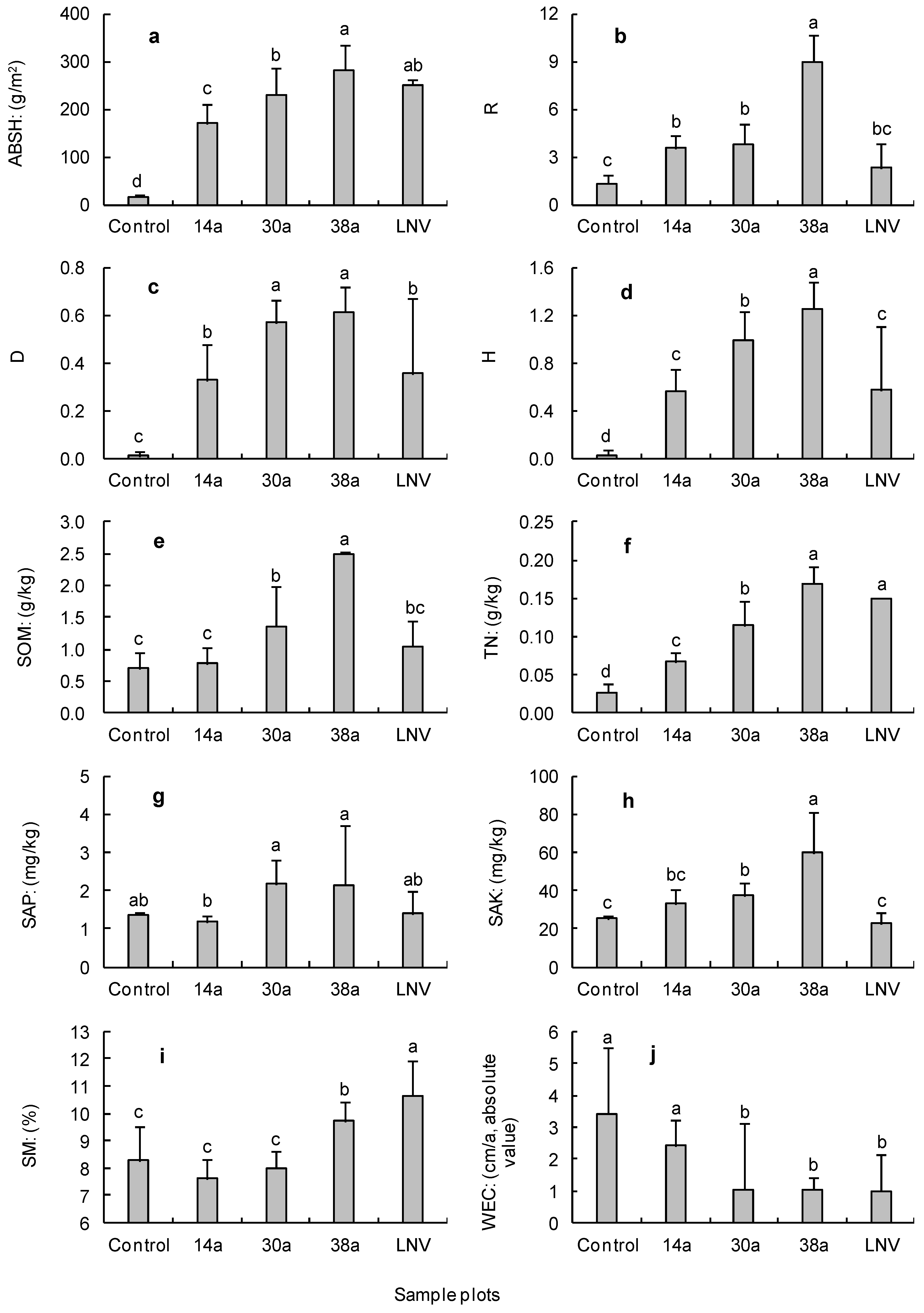
3.2. Ecosystem Services Function Change

As illustrated in Figure 2, all indicators except wind erosion spile height change (WEC) mainly significantly increased with the increase in aerial seeding duration, WEC was the only negative indicator (implying that bigger is worse), in other words, all indicators were moving in the better direction. All indicators except WEC of control were the lowest. In addition, the values of R, D, H, SOM and SAK were significantly higher in 38a than in the local natural vegetation (p < 0.05) (Figure 2b–e,h), the values of SM was significantly lower, while the values of aboveground biomass per unit area of shrub (ABS) + aboveground biomass per unit area of herb (ABH) (ABSH), TN, SAP and WEC were not significantly different (Figure 2a,f,g,j).
When evaluating the ecosystem services function, we can see that the earlier the aerial seeding was conducted, the higher the assessment values were for H. laeve shrubs; the values were 49.02, 82.91 and 96.86 for plots in 14a, 30a and 38a, respectively (Table 4). And as we can see, the assessment value of control was the lowest, only for 29.76, and the values in 38a plots were higher than in the local natural vegetation (81.28).

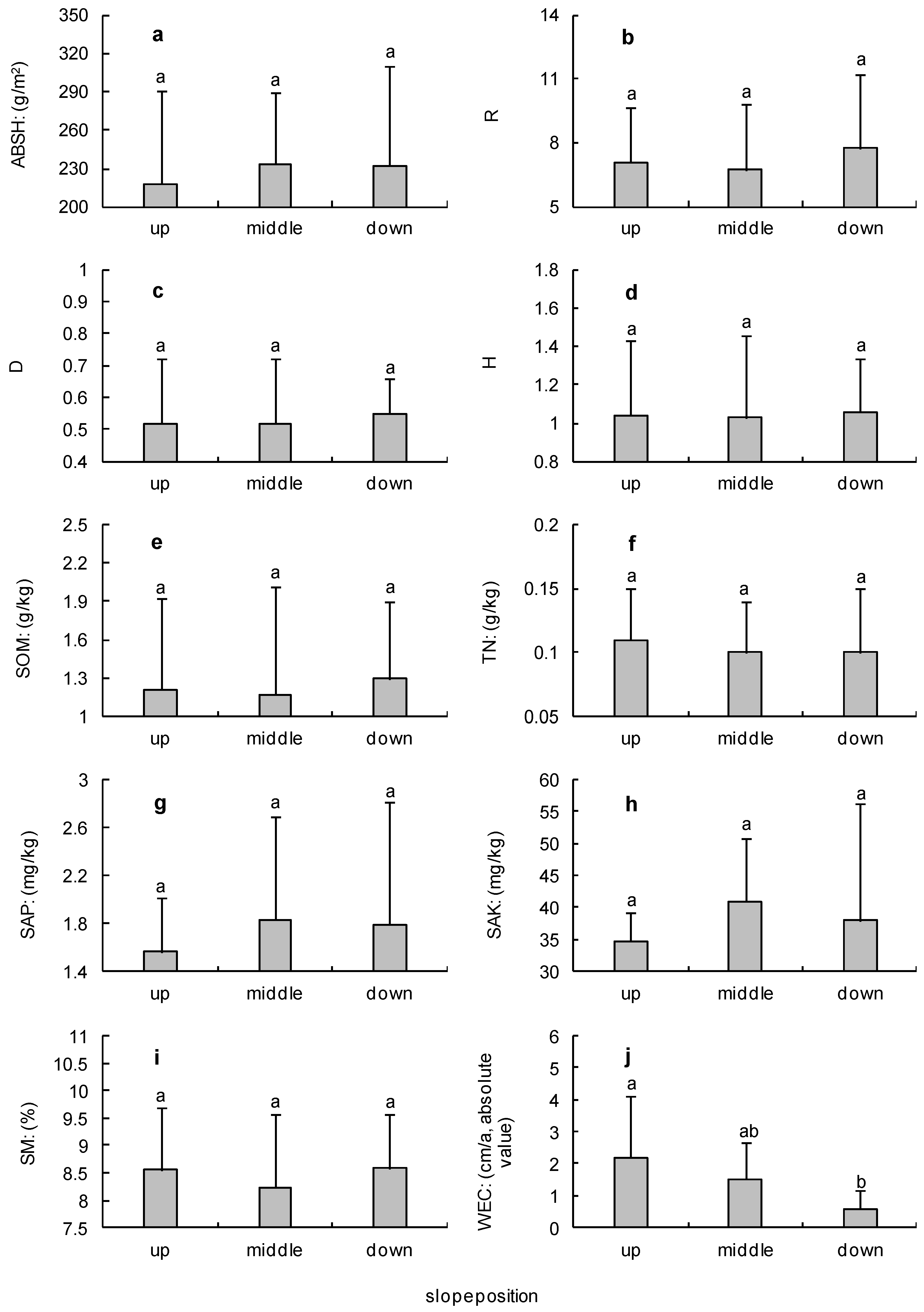
3.3. Ecosystem Service Function at Different Slope Positions

As illustrated in Figure 3, all indicators except WEC mainly increased as the slope position decreased, WEC was the only negative indicator (implying that bigger is worse), in other words, all indicators were moving in the better direction as the slope position decreased. However, the values of ABSH, R, D, H, SOM, TN, SAP, SAK and SM were not significantly different among down-slope, middle-slope and up-slope (Figure 3a–i); only the WEC value was significantly lower at down-slope than at middle-slope (p < 0.05) and was significantly lower at middle-slope than at up-slope (p < 0.05) (Figure 3j). In other words, wind-break and sand-fixation benefits increased as the slope position moved downwards.
The assessment values of H. laeve shrubs increased from 66.90 at the upper end to 99.67 at the lower end of the slope (Table 5).

3.4. Relationships between the Service Indices

There were positive significant correlations between ABSH and R, D, H, SOM, SAK, and SM, between R and D, H, SOM, SAP, SAK, and SM, between D and H, SOM, TN, SAP, and SM, and between H and SOM, TN, SAP, SAK, and SM, but there were negative significant correlations between H and WEC (Table 6). In addition, positive significant correlations were also found between SOM and SAP, SOM and SAK, TN and SM, and SAP and SAK. It was observed that the various relevant diversity indices (R, D, H) were all positively correlated with ABSH, SOM, SAP and SM.

4. Discussion

Ascertaining the direction of vegetation restoration is very important to evaluate whether it is successful. Basically, the native vegetation is one of the key factors which are used to evaluate the success of a restoration [26]. In this study, we revealed a trend of H. laeve being replaced by A. ordosica (Table 3), which is known as the native vegetation [27]. In addition, previous studies had found that increase in nutrient supply enhanced sexual reproduction, but reduced clonal reproduction [28]. In this study, the soil nutrients were increased with the increase in aerial seeding duration (Figure 2e–h), and H. laeve mainly relies on clonal reproduction for population expansion, while A. ordosica relies on sexual reproduction [21], so this could be one of the reasons of H. laeve being replaced by A. ordosica. As time went after the seeding, ecosystem services of H. laeve shrubs increased with the increase in elapsed time since aerial seeding (Figure 2, Table 4), the various relevant diversity indices (R, D, and H) all significantly increased also (Figure 2b–d), and some species, especially grass species, appeared in the herbaceous layer (Table 3). Most important of all, all indicators of aerial seeding were significantly better than the control, and 38a sample plot was even better than the local natural vegetation. Furthermore, without human influence, the control sample was still in the initial stage of succession, the desertification was still under serious conditions (Figure 2j), and there were only two species in the herb layer and even no species in the shrub layer (Table 3). Obviously, aerial seeding of H. laeve was successful and had stimulated succession in Mu Us Sandy Land. Similar results had also been obtained in Australia [29], United States [12,13], Iceland [10] and Canada [30].
Among many other potential reasons for the successful implication of aerial seedling, we want to demonstrate the usage of endemic species, which are well acclimated to the local environment conditions. Besides, using local species can avoid the loss of native species and bring about the threat of invasion when non-native trees are being used [31]. For instance, Cao et al. [16] found that China’s Grain for Green Project, in which non-native trees had been planted in large quantities, had accelerated water shortages and had a negative impact on local biodiversity. Therefore, our results support our first hypothesis that aerial seeding of endemic species can stimulate vegetation succession to local vegetation climax, especially in the adverse environmental conditions, where soil seed banks were scarce.
In this study, as illustrated in Figure 3 and Table 5, the overall values of ecosystem services increased as the slope position decreased, despite the fact that most single index values showed no significant differences (Figure 3). This must be related to the low elevation of the slope not enough to make a significant difference, so our second hypothesis is not true. Compared with mountainous regions [32,33], sandy land as a relatively flat terrain, the relatively smooth topography, however, it can still regulate the hydrothermal processes [34,35]. As we know, water is the most important limiting factor in arid environment, which can promote crust and vegetation growth especially in desert and sandy land [34]. Gamfeldt et al. [36] also indicated that higher levels of multiple ecosystem services were found in forests with more tree species. Thus, the lower end of the slope provides higher levels of ecosystem services, possibly due to the higher biodiversity and soil moisture found down-slope (Figure 3). Similar results were also found on the loess plateau (to the south of our study area) of China [37]. In addition, we explored the relationship between biodiversity and other indices. Isbell et al. [38] confirmed that high plant diversity was needed to maintain ecosystem services. Balvanera et al. [39] also believed that biodiversity generally had a positive impact on ecosystem services. We saw similar results in the aerial seeding of H. laeve in Mu Us Sandy Land, China (Table 6). These could be also the reason that ecosystem services assessment values in 38a sample plot were significantly better than the local natural vegetation (Table 4), because 38a sample plot had higher diversity indices (Figure 2b–d). Therefore, our results are credible in the study area. Given that the relationship between biodiversity and ecosystem functioning has long been topic of concern [40,41,42], there are still many uncertainties due to the complexity of the relationship [15,41,42].
This study has significant practical implications. Our results indicated that the practice of aerial seeding had stimulated vegetation restoration in the Mu Us Sandy Land, China, and indicated positive succession was occurring towards locally native vegetation. Therefore, we propose that aerial seeding of endemic species be generalized to more ecosystems with vegetation degradation problems, where soil seed banks were scarce.

5. Conclusions

To assess the ecosystem service function after different aerial seeding time (14a, 30a, 38a) in Mu Us Sandy Land, we calculated ecosystem service function metrics, including the carbon sequestration ability, biodiversity, physical and chemical properties of soil, and wind-break and sand-fixation on a typical windward slope. The main conclusions are as follows: (1) ecosystem services mainly increased with the number of elapsed years after aerial seeding, and therefore there is no need for human intervention after aerial seeding occurs in the future; (2) the overall assessment values of ecosystem services increased as the slope position moved downwards, despite the fact that most single index values showed no significant differences among the slope positions; and (3) the importance value of H. laeve decreased with increasing years after aerial seeding, while the importance value of A. ordosica increased, indicating that H. laeve was being replaced by A. ordosica, indicating that the vegetation was undergoing a continuous succession towards native climax of vegetation.

Acknowledgments

The research was supported by Special Scientific Research Fund of Forestry Public Welfare Profession of China (201304206), Inner Mongolia Science & Technology Plan of China (201601061), The Natural Science Foundation of Inner Mongolia Autonomous Region of China (2017MS0373 and 2014MS0313).

Author Contributions

Lei Zhang, Xiaojiang Wang and Jie Yang conceived and designed the experiments; Lei Zhang, Guangyu Hong, Zhuofan Li, Xiaowei Gao, Yongzhi Wu and Pingping Wang performed the experiments; Lei Zhang, Guangyu Hong and Zhuofan Li analyzed the data; Xiaojiang Wang and Jie Yang contributed reagents/materials/analysis tools; Lei Zhang wrote the paper.

Conflicts of Interest

The authors declare no conflict of interest.

References

  1. Thomas, D.S.G. Science and the desertification debate. J. Arid Environ. 1997, 37, 599–608. [Google Scholar] [CrossRef]
  2. Bai, Y.F.; Huang, J.H.; Zheng, S.X.; Pan, Q.M.; Zhang, L.X.; Zhou, H.K.; Xu, H.L.; Li, Y.L.; Ma, J. Drivers and regulating mechanisms of grassland and desert ecosystem services. Chin. J. Plant Ecol. 2014, 38, 93–102. (In Chinese) [Google Scholar]
  3. Daily, G.C. Nature’s Services: Societal Dependence on Natural Ecosystems; Island Press: Washington, DC, USA, 1997; ISBN 1-55963-475-8. [Google Scholar]
  4. Balick, M.J.; Elisabetsky, E.; Laird, S.A. Medicinal Resources of the Tropical Forest: Biodiversity and Its Importance to Human Health; Columbia Univ. Press: New York, NY, USA, 1996. [Google Scholar]
  5. Tripathi, K.P.; Singh, B. Species diversity and vegetation structure across various strata in natural and plantation forests in Katerniaghat Wildlife Sanctuary, North India. Trop. Ecol. 2009, 50, 191–200. [Google Scholar]
  6. Shono, K.; Cadaweng, E.A.; Durst, P.B. Application of assisted natural regeneration to restore degraded tropical forestlands. Restor. Ecol. 2007, 15, 620–626. [Google Scholar] [CrossRef]
  7. Orians, G.H.; Pfeiffer, E.W. Ecological effects of the war in Vietnam. Science 1970, 168, 544–554. [Google Scholar] [CrossRef] [PubMed]
  8. Aide, T.M.; Zimmerman, J.K.; Herrera, L.; Rosario, M.; Serrano, M. Forest recovery in abandoned tropical pastures in Puerto Rico. For. Ecol. Manag. 1995, 77, 77–86. [Google Scholar] [CrossRef]
  9. Xiao, X.; Wei, X.H.; Liu, Y.Q.; Ouyang, X.Z.; Li, Q.L.; Ning, J.K. Aerial seeding: An effective forest restoration method in highly degraded forest landscapes of sub-tropic regions. Forests 2015, 6, 1748–1762. [Google Scholar] [CrossRef]
  10. Greipsson, S.; El-Mayas, H. Large-scale reclamation of barren lands in Iceland by aerial seeding. Land Degrad. Dev. 1999, 10, 185–193. [Google Scholar] [CrossRef]
  11. Narita, K.; Wada, N. Ecological significance of the aerial seed pool of a desert lignified annual, Blepharis sindica (Acanthaceae). Plant Ecol. 1998, 135, 177–184. [Google Scholar] [CrossRef]
  12. Davies, K.W.; Bates, J.D.; Madsen, M.D.; Nafus, A.M. Restoration of mountain big sagebrush steppe following prescribed burning to control western juniper. Environ. Manag. 2014, 53, 1015–1022. [Google Scholar] [CrossRef] [PubMed]
  13. Pyke, D.A.; Wirth, T.A.; Beyers, J.L. Does seeding after wildfires in rangelands reduce erosion or invasive species? Restor. Ecol. 2013, 21, 415–421. [Google Scholar] [CrossRef]
  14. Clements, W.H.; Vieira, N.K.M.; Church, S.E. Quantifying restoration success and recovery in a metal-polluted stream: A 17-year assessment of physicochemical and biological responses. J. Appl. Ecol. 2010, 47, 899–910. [Google Scholar] [CrossRef]
  15. Bullock, J.M.; Aronson, J.; Newton, A.C.; Pywell, R.F.; Reybenayas, J.M. Restoration of ecosystem services and biodiversity: Conflicts and opportunities. Trends Ecol. Evol. 2011, 26, 541–549. [Google Scholar] [CrossRef] [PubMed]
  16. Cao, S.X.; Chen, L.; Yu, X.X. Impact of China’s Grain for Green Project on the landscape of vulnerable arid and semi-arid agricultural regions: A case study in northern Shaanxi Province. J. Appl. Ecol. 2009, 46, 536–543. [Google Scholar] [CrossRef]
  17. Chazdon, R.L. Beyond deforestation: Restoring forests and ecosystem services on degraded lands. Science 2008, 320, 1458–1460. [Google Scholar] [CrossRef] [PubMed]
  18. Zhang, X.S. Principles and optimal models for development of Maowusu sandy grassland. Acta Ecol. Sin. 1994, 18, 1–16. (In Chinese) [Google Scholar]
  19. Tiemuer, B.; Tana; Hasi, M.; Huang, S.R. The development current situation and future development advice of the shrubbery in Wushen country. Prot. For. Sci. Technol. 2014, 124, 75–76. (In Chinese) [Google Scholar]
  20. Hein, L.; van Koppenb, K.; de Groot, R.S.D.; van Ierland, E.C. Spatial scales, stakeholders and the valuation of ecosystem services. Ecol. Econ. 2006, 57, 209–228. [Google Scholar] [CrossRef]
  21. Liu, F.H.; Ye, X.H.; Yu, F.H.; Dong, M. Clonal integration modifies responses of Hedysarum Laeve to local sand burial in Mu Us Sandland. Chin. J. Plant Ecol. 2006, 30, 278–285. (In Chinese) [Google Scholar]
  22. Xie, Y.Z.; Qiu, K.Y.; Xu, D.M.; Shi, X.F.; Qi, T.Y.; Richard, P. Spatial heterogeneity of soil and vegetation characteristics and soil-vegetation relationships along an ecotone in southern Mu Us Sandy Land, China. J. Soil Sediment 2015, 15, 1584–1601. [Google Scholar] [CrossRef]
  23. Wang, B.; Yang, F.W.; Guo, H.; Li, S.N.; Wang, Y.; Ma, X.Q.; Yu, X.X.; Lu, S.W.; Wang, H.W.; Wei, W.J. Specifications for Assessment of Forest Ecosystem Services in China; LY/T1721-2008; Standards Press of China: Beijing, China, 2008. (In Chinese) [Google Scholar]
  24. Ramanathan, R. A note on the use of the analytic hierarchy process for environmental impact assessment. J. Environ. Manag. 2001, 63, 27–35. [Google Scholar] [CrossRef] [PubMed]
  25. Nekooee, Z.; Karami, M.; Fakhari, I. Assessment and prioritization of urban tourist attractions based on analytical hierarchy process (AHP) (a case study of Birjand, Iran). Ecography 2011, 35, 65–72. [Google Scholar]
  26. Wilcox, J.C.; Healy, M.T.; Zedler, J.B. Restoring native vegetation to an urban wet meadow dominated by reed canarygrass (Phalaris arundinacea L.) in Wisconsin. Nat. Area J. 2015, 27, 354–365. [Google Scholar] [CrossRef]
  27. Shen, W.S. Successional Stage and rate of the aerial seeding vegetation in the Maowusu Sandyland. Sci. Silvae Sin. 1999, 35, 103–108. (In Chinese) [Google Scholar] [CrossRef]
  28. Zhu, Y.J.; Alaten, B.; Dong, M.; Huang, Z.Y. Effects of increasing water or nutrient supplies on reproduction trade-offs in the natural populations of clonal plant, Hedysarum laeve. Chin. J. Plant Ecol. 2007, 31, 658–664. (In Chinese) [Google Scholar]
  29. Bassett, O.D.; Prior, L.D.; Slijkerman, C.M.; Jamieson, D.; Bowman, D.M.J.S. Aerial sowing stopped the loss of alpine ash (Eucalyptus delegatensis) forests burnt by three short-interval fires in the Alpine National Park, Victoria, Australia. For. Ecol. Manag. 2015, 342, 39–48. [Google Scholar] [CrossRef]
  30. McLaughlin, B.E.; Crowder, A.A. The distribution of Agrostis gigantea and Poa pratensis in relation to some environmental factors on a mine-tailings area at Copper Cliff, Ontario. Can. J. Bot. 1988, 66, 2317–2322. [Google Scholar] [CrossRef]
  31. Nehring, S.; Hesse, K.J. Invasive alien plants in marine protected areas: The Spartina anglica affair in the European Wadden Sea. Biol. Invasions 2008, 10, 937–950. [Google Scholar] [CrossRef]
  32. Del Barrio, G.; Alvera, B.; Puigdefabregas, J.; Diez, C. Response of high mountain landscape to topographic variables: Central Pyrenees. Landsc. Ecol. 1997, 12, 95–115. [Google Scholar] [CrossRef]
  33. Tatian, M.; Arzani, H.; Reihan, M.K.; Bahmanyar, M.A.; Jalilvand, H. Effect of soil and physiographic factors on ecological plant groups in the eastern Elborz mountain rangeland of Iran. Grassl. Sci. 2010, 56, 77–86. [Google Scholar] [CrossRef]
  34. Kidron, G.J. Differential water distribution over dune slopes as affected by slope position and microbiotic crust, Negev Desert, Israel. Hydrol. Process 1999, 13, 1665–1682. [Google Scholar] [CrossRef]
  35. Nagamatsu, D.; Hirabuki, Y.; Mochida, Y. Influence of micro-landforms on forest structure, tree death and recruitment in a Japanese temperate mixed forest. Ecol. Res. 2003, 18, 533–547. [Google Scholar] [CrossRef]
  36. Gamfeldt, L.; Snäll, T.; Bagchi, R.; Jonsson, M.; Gustafsson, L.; Kjellander, P.; Ruiz-Jaen, M.C.; Fröberg, M.; Stendahl, J.; Philipson, C.D.; et al. Higher levels of multiple ecosystem services are found in forests with more tree species. Nat. Commun. 2011, 4, 1–8. [Google Scholar] [CrossRef] [PubMed] [Green Version]
  37. Feng, Q.; Zhao, W.W.; Fu, B.J.; Ding, J.Y.; Wang, S. Ecosystem service trade-offs and their influencing factors: A case study in the Loess Plateau of China. Sci. Total Environ. 2017, 607–608, 1250–1263. [Google Scholar] [CrossRef] [PubMed]
  38. Isbell, F.; Calcagno, V.; Hector, A.; Connolly, J.; Harpole, W.S.; Reich, P.B.; Scherer-Lorenzen, M.; Schmid, B.; Tilman, D.; van Ruijven, J.; et al. High plant diversity is needed to maintain ecosystem services. Nature 2011, 477, 199–202. [Google Scholar] [CrossRef] [PubMed] [Green Version]
  39. Balvanera, P.; Pfisterer, A.B.; Buchmann, N.; He, J.S.; Nakashizuka, T.; Raffaelli, D.; Schmid, B. Quantifying the evidence for biodiversity effects on ecosystem functioning and services. Ecol. Lett. 2006, 9, 1146–1156. [Google Scholar] [CrossRef] [PubMed] [Green Version]
  40. Bu, W.S.; Zang, R.G.; Ding, Y. Field observed relationships between biodiversity and ecosystem functioning during secondary succession in a tropical lowland rainforest. Acta Oecol. 2014, 55, 1–7. [Google Scholar] [CrossRef]
  41. Mace, G.M.; Norris, K.; Fitter, A.H. Biodiversity and ecosystem services: A multilayered relationship. Trends Ecol. Evol. 2012, 27, 19–26. [Google Scholar] [CrossRef] [PubMed]
  42. Luck, G.W.; Daily, G.C.; Ehrlich, P.R. Population diversity and ecosystem services. Trends Ecol. Evol. 2003, 18, 331–336. [Google Scholar] [CrossRef]
Figure 1. The geographic location and photos of the sample plots.
Sustainability 10 00902 g001
Figure 2. (a) Changes of ABSH (Aboveground biomass per unit area of shrub (ABS) + Aboveground biomass per unit area of herb (ABH)) of the sample plots; (b) Changes of R (Richness index) of the sample plots; (c) Changes of D (Simpson index) of the sample plots; (d) Changes of H (Shannon–Wiener index) of the sample plots; (e) Changes of SOM (Soil organic matter) of the sample plots; (f) Changes of TN (Total nitrogen) of the sample plots; (g) Changes of SAP (Soil available phosphorus) of the sample plots; (h) Changes of SAK (Soil available potassium) of the sample plots; (i) Changes of SM (Soil moisture) of the sample plots; (j) Changes of WEC (Wind erosion spile height change) of the sample plots; LNV means local natural vegetation.
Sustainability 10 00902 g002
Figure 3. (a) Changes of ABSH (Aboveground biomass per unit area of shrub (ABS) + Aboveground biomass per unit area of herb (ABH)) at different slope positions for H. laeve shrubs; (b) Changes of R (Richness index) at different slope positions for H. laeve shrubs; (c) Changes of D (Simpson index) at different slope positions for H. laeve shrubs; (d) Changes of H (Shannon–Wiener index) at different slope positions for H. laeve shrubs; (e) Changes of SOM (Soil organic matter) at different slope positions for H. laeve shrubs; (f) Changes of TN (Total nitrogen) at different slope positions for H. laeve shrubs; (g) Changes of SAP (Soil available phosphorus) at different slope positions for H. laeve shrubs; (h) Changes of SAK (Soil available potassium) at different slope positions for H. laeve shrubs; (i) Changes of SM (Soil moisture) at different slope positions for H. laeve shrubs; (j) Changes of WEC (Wind erosion spile height change) at different slope positions for H. laeve shrubs.
Sustainability 10 00902 g003
Table 1. Basic conditions of sample plots in Mu Us Sandy Land, China.
Sample PlotGeographical Position (Latitude and Longitude)Altitude (m)Aerial Seeding SpeciesSite Types before Aerial SeedingSeeding Density (kg/hm2)Area (hm2)
Elapsed time after aerial seeding (a)
14 (in 2002)N:38°51′
E:109°15′
1309H. laeveMoving and semi-moving sandy land8–9667
30 (in 1986)N:39°23′
E:109°50′
1329H. laeveMoving and semi-moving sandy land8–9333
38 (in 1978)N:39°08′
E:109°31′
1350H. laeveMoving and semi-moving sandy land8–9667
Others
ControlN:39°07′
E:109°27′
1391Not ImplementedMoving and semi-moving sandy land in 1978//
Local natural vegetationN:38°52′
E:109°13′
1306Not ImplementedAlways been A. ordosica community//
Table 2. Ecosystem service function assessment system.
Total Target LayerCriteria LayerWeightIndex LayerWeightCombined WeightIndex Attribute
A
Ecosystem service function assessment
B1 Carbon sequestration ability0.08C1 Aboveground biomass per unit area of shrub (ABS) + Aboveground biomass per unit area of herb (ABH) (ABSH)1.000.0833positive
B2 Biodiversity0.25C2 Richness index (R)0.330.0833positive
C3 Simpson index (D)0.330.0833positive
C4 Shannon–Wiener index (H)0.330.0833positive
B3 Soil fertility0.08C5 Soil organic matter (SOM)0.500.0417positive
C6 Total nitrogen (TN)0.250.0208positive
C7 Soil available phosphorus (SAP)0.130.0104positive
C8 Soil available potassium (SAK)0.130.0104positive
B4 Water conservation functions0.17C9 Soil moisture (SM)1.000.1667positive
B5 Wind-break and sand-fixation0.42C10 Wind erosion spile height change (WEC)1.000.4167negative
“Positive” means that the bigger the better, and “negative” means that the bigger the worse. The values of weight and combined weight are the result of the expert survey.
Table 3. Plant species importance values (IVs) of sample plots in Mu Us Sandy Land, China.
SpeciesControlElapsed Time after Aerial Seeding (a)Local Natural Vegetation
143038
Shrub layer
H. laeve Maxim.-0.9502 0.6255 0.4994 -
A. ordosica Krasch-0.0498 0.3745 0.5006 1.0000
Herb layer
Bassia dasyphylla (Fisch. et Mey.) O. Kuntze0.0858 0.4644 0.0449 0.0245 -
Corispermum mongolicum Iljin0.9142 0.3471 0.1849 -0.5620
Ixeridium graminifolium (Ledeb.) Tzvel.-0.1123 0.0105 0.0431 0.0569
Setaria viridis (L.) Beauv.-0.0319 0.2553 --
Incarvillea sinensis Lam.-0.0177 ---
Cynanchum thesioides (Freyn) K. Schum.-0.0098 -0.0077 0.0813
Sonchus brachyotus DC.-0.0091 ---
Heteropappus altaicus (Willd.) Novopokr.-0.0078 -0.0409 -
Euphorbia humifusa Willd. ex Schlecht.--0.1557 --
Chenopodium aristatum L.--0.1444 --
Chenopodium glaucum L.--0.1364 0.0084 -
Euphorbia esula L.--0.0449 0.0388 -
Silene jenisseensis Willd.--0.0101 0.0222 -
Poa sphondylodes Trin.--0.0130 --
Artemisia hedinii Ostenf. et Pauls.---0.0188 -
Eragrostis minor Host---0.0448 0.0569
Allium mongolicum Regel---0.0374 -
Leontopodium leontopodioides (Willd. ) Beauv.---0.0215 -
Leymus chinensis (Trin.) Tzvel.---0.5117 0.2429
Tribulus terrester L.---0.0060 -
Cynanchum hancockianum (Maxim.) Al. Iljinski---0.0398 -
Artemisia sphaerocephala Krasch.---0.0191 -
Inula salsoloides (Turcz. ) Ostenf.---0.0263 -
Thalictrum petaloideum L.---0.0691 -
Salsola collina Pall.---0.0200 -
Table 4. Ecosystem services function dimensionless values and assessment results of sample plots in Mu Us Sandy Land, China.
Index ControlElapsed Time after Aerial Seeding (a)Local Natural Vegetation
143038
C1 ABSH6.27 60.50 81.69 100.00 89.23
C2 R14.81 39.81 42.59 100.00 25.93
C3 D1.87 53.74 92.95 100.00 58.31
C4 H2.34 45.10 79.25 100.00 45.95
C5 SOM27.96 31.03 54.23 100.00 41.93
C6 TN15.99 39.99 67.74 100.00 88.43
C7 SAP63.83 54.74 100.00 99.17 64.83
C8 SAK42.11 54.94 62.49 100.00 38.14
C9 SM77.49 71.52 75.15 91.27 100.00
C10 WEC29.13 41.38 96.77 96.00 100.00
Assessment Value (Xi)29.76 49.02 82.91 96.86 81.28
Table 5. Dimensionless values and assessment results of ecosystem service function at different slope positions in Mu Us Sandy Land, China.
Index Slope Positions
UpMiddleDown
C1 ABSH 93.49 100.00 99.62
C2 R91.35 87.10 100.00
C3 D94.55 94.55 100.00
C4 H98.11 97.17 100.00
C5 SOM93.80 90.70 100.00
C6 TN100.00 90.91 90.91
C7 SAP85.25 100.00 97.81
C8 SAK84.75 100.00 92.75
C9 SM99.65 96.04 100.00
C10 WEC26.61 37.91 100.00
Assessment Value (Xi)66.90 71.11 99.67
Table 6. Pearson correlation coefficients between the ecosystem function service indices in Mu Us Sandy Land, China.
ABSHRDHSOMTNSAPSAKSMWEC
ABSH1
R0.651 **1
D0.371 *0.387 *1
H0.441 **0.529 **0.959 **1
SOM0.429 *0.711 **0.532 **0.652 **1
TN0.1850.2580.599 **0.610 **0.2651
SAP0.3250.418 *0.479 *0.545 **0.506 **0.3911
SAK0.399 *0.676 **0.3340.423 *0.600 **0.2670.490 **1
SM0.439 **0.667 **0.471 **0.524 **0.3760.406*0.0950.121
WEC−0.273−0.321−0.215−0.342 *−0.277−0.178−0.353−0.269−0.1731
* P < 0.05, ** P < 0.01 (two-tailed). ABSH (Aboveground biomass per unit area of shrub (ABS) + Aboveground biomass per unit area of herb (ABH)), R (Richness index), D (Simpson index), H (Shannon–Wiener index), SOM (Soil organic matter), TN (Total nitrogen), SAP (Soil available phosphorus), SAK (Soil available potassium), SM (Soil moisture), WEC (Wind erosion spile height change).

