Forecasting of Energy-Related CO₂ Emissions in China Based on GM(1,1) and Least Squares Support Vector Machine Optimized by Modified Shuffled Frog Leaping Algorithm for Sustainability

Abstract

Presently, China is the largest CO₂ emitting country in the world, which accounts for 28% of the CO₂ emissions globally. China’s CO₂ emission reduction has a direct impact on global trends. Therefore, accurate forecasting of CO₂ emissions is crucial to China’s emission reduction policy formulating and global action on climate change. In order to forecast the CO₂ emissions in China accurately, considering population, the CO₂ emission forecasting model using GM(1,1) (Grey Model) and least squares support vector machine (LSSVM) optimized by the modified shuffled frog leaping algorithm (MSFLA) (MSFLA-LSSVM) is put forward in this paper. First of all, considering population, per capita GDP, urbanization rate, industrial structure, energy consumption structure, energy intensity, total coal consumption, carbon emission intensity, total imports and exports and other influencing factors of CO₂ emissions, the main driving factors are screened according to the sorting of grey correlation degrees to realize feature dimension reduction. Then, the GM(1,1) model is used to forecast the main influencing factors of CO₂ emissions. Finally, taking the forecasting value of the CO₂ emissions influencing factors as the model input, the MSFLA-LSSVM model is adopted to forecast the CO₂ emissions in China from 2018 to 2025.

1. Introduction

With the continuous progress of human society and global industrialization, the consumption of fossil fuels is getting faster and faster, resulting in serious environmental problems, such as the greenhouse effect. CO₂ is one of the main gases that cause the greenhouse effect. Carbon capture and storage is the process of capturing and storing the CO₂ in industrial production by various means, such as cryogenic carbon capture [1,2], chemical absorption [3], oxyfuel combustion [4] and so on. Carbon capture technologies that result in significant reduction in energy-related CO₂ emissions, specifically from coal-fired power plants, can relieve the greenhouse effect. The economic efficiency and feasibility of these carbon capture technologies are affected by CO₂ emission forecasting. Presently, China is the largest CO₂ emitting country in the world, which accounts for 28% of the CO₂ emissions globally. China’s CO₂ emission reduction has a direct impact on global trends. Therefore, accurate forecasting of CO₂ emissions is crucial to China’s emission reduction policy formulating and global action on climate change.

Currently, scholars have put forward various models for CO₂ emission forecasting, such as multiple linear regression [5,6,7], system dynamics [8,9,10] and grey model [11,12]. Matjafri and Lim [13] proposed the forecasting model to predict the CO₂ emissions in Malaysia. They removed irrelevant data by the best subset method and built the prediction model of multi linear regression. Zhong [14] forecasted CO₂ emissions and energy demand with the system dynamics approach through mode analyzing of energy consumption and population and economic development and proposed suggestions for energy development. The grey forecasting model was used by Lin et al. [15] to estimate CO₂ emissions from 2010 to 2012 in Taiwan. The forecasting results showed that the mean residual error of the GM(1,1) was less than 10%, and CO₂ emissions in Taiwan over the next 3 years would increase.

Recently, with the continuous development of artificial intelligence technology, more and more intelligent forecasting models are applied to the field of prediction, which is also suitable for the forecasting of CO₂ emissions. The neural network model [16,17,18] and support vector machine [19,20] are two widely used artificial intelligence forecasting models. Gallo et al. [21] put forward the artificial neural network model which had a more flexible system to predict short-term CO₂ emissions instead of classical methods. Combined with the rough set and the grey system model and support vector machine, Zhou and Zhang [22] proposed the model to forecast the CO₂ emissions in China using the data of the population, gross domestic product (GDP) and total energy consumption.

Compared with the neural network algorithm, SVM has superior generalization, which can better refrain from the local optimum by parameter optimization. The least squares support vector machine (LSSVM) [23,24,25] is an improved algorithm based on equality constraint and least squares value function for standard SVM. LSSVM uses the quadratic loss function to transform the secondary optimization of SVM algorithm into the solution of linear equation, which has better convergence accuracy and a faster training speed. Therefore, LSSVM is used to forecast CO₂ emissions in this article. At present, for the parameter optimization of LSSVM, researchers have proposed various optimization algorithms, such as PSO (particle swarm optimization) [26,27], GA (genetic algorithm) [28,29], and ABC (artificial bee colony) [30,31,32]. Wang et al. [33] proposed a short-term load prediction model based on LSSVM optimized by improved parallel PSO to improve the accuracy of load forecasting. Wen et al. [34] proposed the LSSVM model with genetic algorithm to forecast landslide displacement and used a case study to prove that the GA-LSSVM model was effective for the prediction of landslide displacement. Mustaffa and Yusof [35] put forward the LSSVM model to forecast gold price, and the artificial bee colony intelligent technology was used to obtain the ideal value of parameters of LSSVM. Through empirical analysis, it was proved that the ABC-LSSVM model was a promising approach for financial forecasting. In this paper, shuffled frog leaping algorithm (SFLA) is used to realize the optimization of LSSVM. SFLA simulates the behavior of information exchange in each frog group for food searching. It is a new heuristic colony evolution algorithm, which has efficient calculated performance and excellent global search ability [36,37,38,39].

In this article, for forecasting the CO₂ emissions in China more accurately, a novel forecasting model is proposed based on the main driving factors of CO₂ emissions. The major innovations of this paper are as follows:

(1)

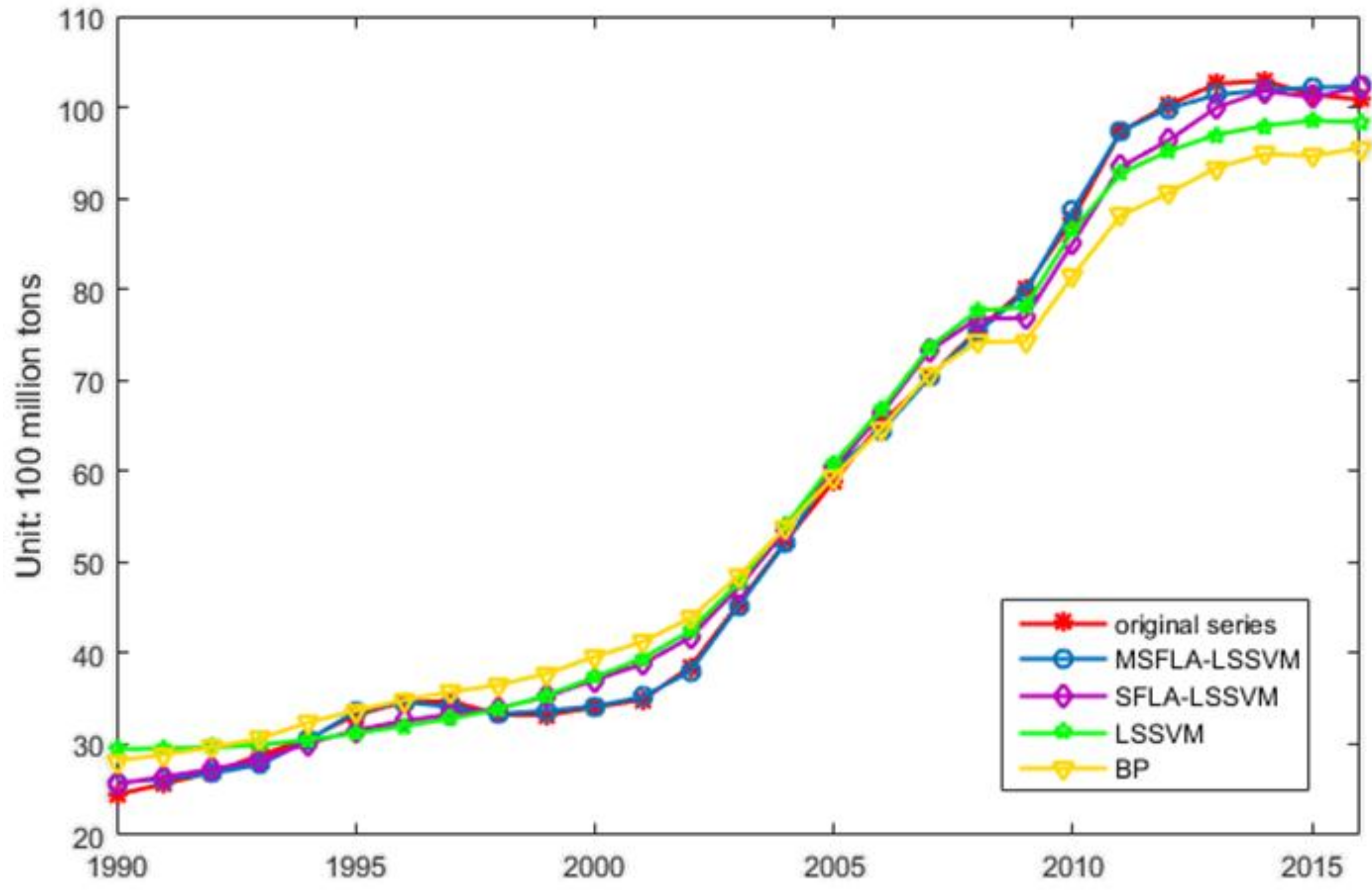
In this paper, the CO₂ emissions forecasting model based on GM(1,1) and LSSVM optimized by MSFLA (MSFLA-LSSVM) are put forward. First of all, the GM(1,1) model is used to forecast the main influencing factors of CO₂ emissions. Then, the MSFLA-LSSVM model is adopted to forecast the CO₂ emissions taking the forecasting value of the CO₂ emissions influencing factors as the model input. Finally, through empirical analysis, it is verified that the MSFLA-LSSVM model has strong generalization ability and robustness for CO₂ emission forecasting and the forecasting accuracy of MSFLA-LSSVM is better than that of SFLA-LSSVM, LSSVM and BP (back propagation) neural network models, which can achieve good forecasting results.

(2)

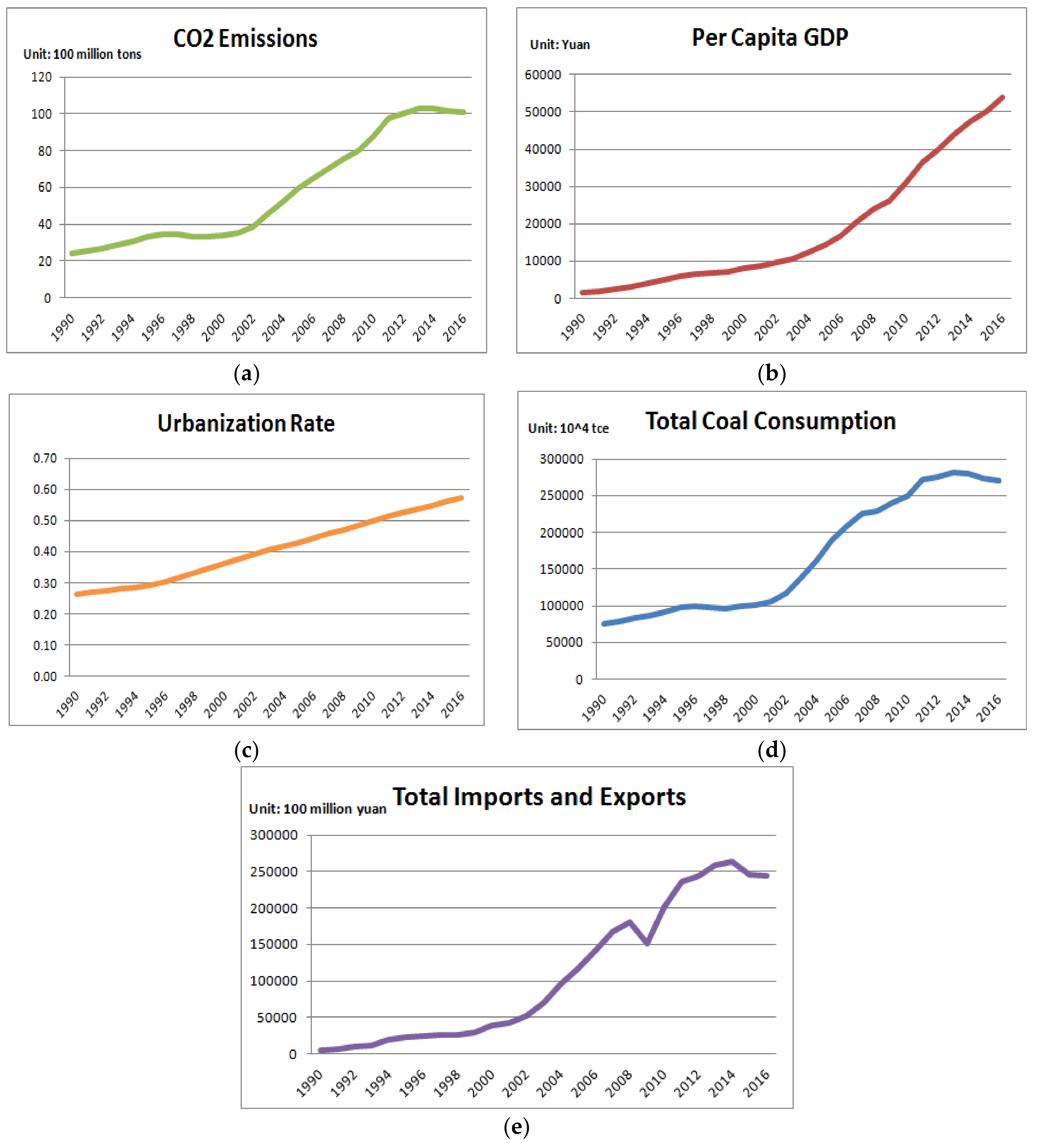
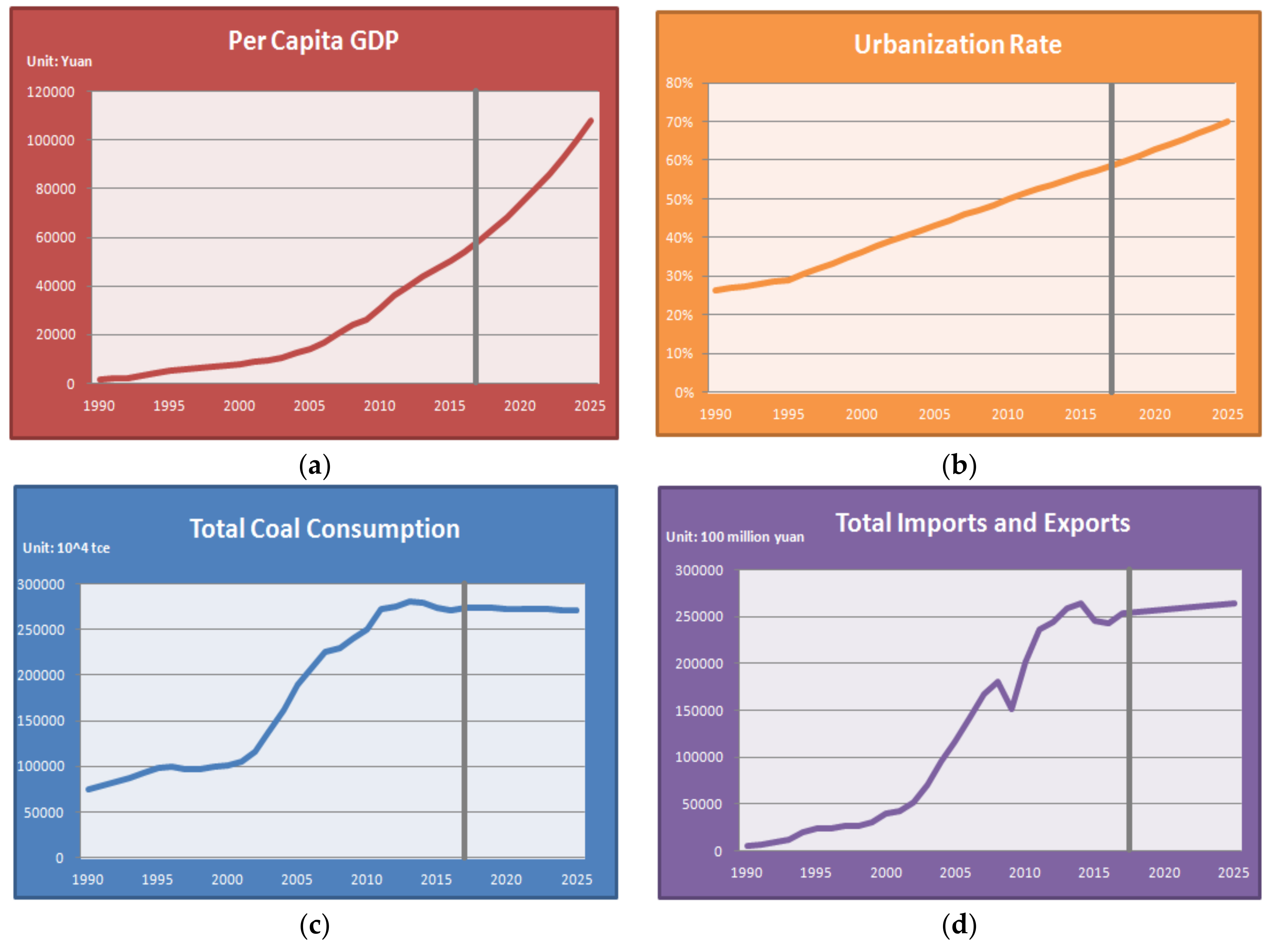
The forecasting accuracy of CO₂ emissions is affected by many factors. Considering population, per capita GDP, urbanization rate, industrial structure, energy consumption structure, energy intensity, total coal consumption, carbon emissions intensity, total imports and exports and other influencing factors of CO₂ emissions, the main driving factors of CO₂ emissions are screened as the model input according to the sorting of grey relational degrees to realize feature dimension reduction.

The main structure and contents of this article are as follows: the second section introduces the forecasting model of GM(1,1) and LSSVM optimized by MSFLA (MSFLA-LSSVM). The third section carries out empirical analysis to prove the practicality and validity of the proposed model for CO₂ emissions forecasting, and forecasts the CO₂ emissions in China from 2018 to 2025. The fourth section summarizes the full text.

2. The Forecasting Model

2.1. GM(1,1)

The model of GM(1,1) is the most commonly applied grey model, which consists of a first order differential equation containing only one variable. The model is simple to calculate and has obvious advantages for the forecasting of small sample data with irregular distribution [11,12]. The specific mathematical model of GM(1,1) is as follows:

Set $x^{(0)}$ as the original sequence:

$$x^{(0)}=\left[x^{(0)}(1),x^{(0)}(2),\cdots ,x^{(0)}(n)\right].$$

(1)

The accumulated generating operation of $x^{(0)}$ is made, and the sequence $x^{(1)}$ is obtained:

$$x^{(1)}=\left[x^{(1)}(1),x^{(1)}(2),\cdots ,x^{(1)}(n)\right].$$

(2)

where $x^{(1)}(k)={\displaystyle \sum _{i=1}^k{x}^{(0)}(i)}$, $k=1,2,\cdots ,n$. $x^{(1)}(k)$ satisfies the following first order linear differential equation model:

$$\frac{d{x}^{(1)}}{dt}+a{x}^{(1)}=u.$$

(3)

In the equation, $a$ and $u$ are parameters to be estimated. According to the definition of derivative:

$$\frac{d{x}^{(1)}}{dt}=\underset{\Delta t\to o}{\lim }\frac{x^{(1)}(t+\Delta t)-x^{(1)}(t)}{\Delta t}.$$

(4)

If expressed in the discrete form, the differential term can be written as:

$$\begin{array}{ll}\frac{\Delta x^{(1)}}{\Delta t}=\frac{x^{(1)}(k+1)-x^{(1)}(k)}{k+1-k}& =x^{(1)}(k+1)-x^{(1)}(k)\\ & ={\alpha }^{(1)}\left[x^{(1)}(k+1)\right]=x^{(0)}(k+1).\end{array}$$

(5)

where $x^{(1)}$ takes the mean of time $k$ and $k+1$, that is $\frac{1}{2}\left[x^{(1)}(k+1)+x^{(1)}(k)\right]$. Therefore, Equation (5) can be rewritten as:

$${\alpha }^{(1)}\left[x^{(1)}(k+1)\right]+\frac{1}{2}a\left[x^{(1)}(k+1)+x^{(1)}(k)\right]=u.$$

(6)

The following equation can be derived:

$$\begin{array}{l}k=1,x^{(0)}(2)+\frac{1}{2}a\left[x^{(1)}(1)+x^{(1)}(2)\right]=u,\\ k=2,x^{(0)}(3)+\frac{1}{2}a\left[x^{(1)}(2)+x^{(1)}(3)\right]=u,\\ \hfill ⋮\hfill \\ k=n-1,x^{(0)}(n)+\frac{1}{2}a\left[x^{(1)}(n)+x^{(1)}(n-1)\right]=u.\end{array}$$

(7)

The above results are expressed in matrix form:

$$\left(\begin{array}{c}{x}^{(0)}(2)\\ x^{(0)}(3)\\ ⋮\\ x^{(0)}(n)\end{array}\right)=\left(\begin{array}{cc}-\frac{1}{2}\left[x^{(1)}(1)+x^{(1)}(2)\right]& 1\\ -\frac{1}{2}\left[x^{(1)}(2)+x^{(1)}(3)\right]& 1\\ ⋮& ⋮\\ -\frac{1}{2}\left[x^{(1)}(n-1)+x^{(1)}(n)\right]& 1\end{array}\right)\left(\begin{array}{c}a\\ u\end{array}\right).$$

(8)

Equation (8) can be written as:

$$Y_n=BA,Y_n=\left(\begin{array}{c}{x}^{(0)}(2)\\ x^{(0)}(3)\\ ⋮\\ x^{(0)}(n)\end{array}\right),A=\left(\begin{array}{c}a\\ u\end{array}\right),B=\left(\begin{array}{cc}-\frac{1}{2}\left[x^{(1)}(1)+x^{(1)}(2)\right]& 1\\ -\frac{1}{2}\left[x^{(1)}(2)+x^{(1)}(3)\right]& 1\\ ⋮& ⋮\\ -\frac{1}{2}\left[x^{(1)}(n-1)+x^{(1)}(n)\right]& 1\end{array}\right).$$

(9)

$Y_n$ and $B$ are known quantities. $A$ is the parameter to be estimated. According to the least squares criterion, Equation (9) can be rewritten as:

$$Y_n=B\widehat{A}+E.$$

(10)

where $E$ is an error term. Let $\min {\Vert Y_n-B\widehat{A}\Vert }^2=\min {(Y_n-B\widehat{A})}^T(Y_n-B\widehat{A})$, the following equation can be obtained according to the matrix derivation equation:

$$\widehat{A}={(B^{T}B)}^{-1}{B}^{T}Yn=\left(\begin{array}{c}\widehat{a}\\ \widehat{u}\end{array}\right).$$

(11)

The parameters in the original differential equation are replaced by $\widehat{a}$ and $\widehat{u}$:

$$\frac{d{x}^{(1)}}{dt}+\widehat{a}{x}^{(1)}=\widehat{u}.$$

(12)

$x^{(1)}(t+1)$ can be solved by the above equation:

$$x^{(1)}(t+1)=\left[x^{(1)}(1)-\frac{\widehat{u}}{\widehat{a}}\right]e^{-\widehat{a}t}+\frac{\widehat{u}}{\widehat{a}}.$$

(13)

$x^{(1)}(1)=x^{(0)}(1)$ is known. Express Equation (13) as the discrete form and Equation (14) is obtained:

$$x^{(1)}(k+1)=\left[x^{(0)}(1)-\frac{\widehat{u}}{\widehat{a}}\right]e^{-\widehat{a}k}+\frac{\widehat{u}}{\widehat{a}}(k=0,1,2\cdots ).$$

(14)

Equations (13) and (14) are the time response functions of GM(1,1). The cumulative reduction of Equation (14) is made, and the gray forecasting model of the original sequence $x^{(0)}$ is obtained:

$$\begin{array}{ll}{\widehat{x}}^{(0)}(k+1)& ={\widehat{x}}^{(1)}(k+1)-{\widehat{x}}^{(1)}(k)\\ & =(1-e^{\widehat{a}})(x^{(0)}(1)-\frac{\widehat{u}}{\widehat{a}})e^{-\widehat{a}k}(k=0,1,2\cdots ).\end{array}$$

(15)

2.2. LSSVM

Let $N$ be the sample number and $m$ be the dimension of sample space. For training samples $(x_i,y_i),i=1,2,\cdots ,N$, there is a nonlinear mapping $\phi (x)$, which can map the samples to high dimensional linear space:

$$f(x)=\omega \phi (x)+b.$$

(16)

According to the principle of structural risk minimization, the above problem can be equivalent to quadratic programming problem as follows:

$$\begin{array}{l}\underset{\omega ,b,\epsilon }{\min }J(\omega ,\epsilon )=\frac{1}{2}{\omega }^T\omega +\frac{1}{2}\xi {\displaystyle \sum _{i=1}^N{\epsilon }_i^2}.\\ s.t.y_i=\omega \phi (x)+b+{\epsilon }_i,i=1,2,\cdots ,N.\end{array}$$

(17)

In the equation, $J(\omega ,\epsilon )$ is structural risk. $\xi$ is penalty coefficient. ${\epsilon }_i$ is allowable error and ${\omega }^T\omega$ controls the model generalization ability. The Lagrange method is adopted to solve the optimization problem of Equation (17). According to Karush–Kuhn–Tucker optimization conditions, the following can be obtained:

$$\left[\begin{array}{cc}0& 1_N^T\\ 1_N& \theta +\frac{1}{\xi }{I}_N\end{array}\right]\left[\begin{array}{c}b\\ a\end{array}\right]=\left[\begin{array}{c}0\\ y\end{array}\right].$$

(18)

In the equation, $y={\left[y_1,y_2,\cdots ,y_N\right]}^T$, $1_N={\left[1,1,\cdots ,1\right]}^T$, $1_N$ is unit matrix. The kernel function is defined according to the Mercer condition:

$$K(x_i,x_j)=\phi {(x_i)}^T\phi (x_j).$$

(19)

The output of the least squares support vector machine can be obtained:

$$f(x)={\displaystyle \sum _{i=1}^N{\alpha }_{i}K(x,x_i)}+b.$$

(20)

2.3. Modified Shuffled Frog Leaping Algorithm

2.3.1. SFLA

The mathematical modeling process of SFLA is as follows:

Generate frog populations $S$ randomly. The frog number in the population is $N$, $S=(X_1,X_2,\cdots ,X_N)$. If the dimension of the candidate solution $X_i$ is $t$, the $j$ candidate solution can be expressed as $X_j=(x_{j1},x_{j2},\cdots ,x_{jt}),0\le j\le N$. The fitness value $f(X_i)$ of each frog is calculated, and frog individuals (candidate solutions) are ranked in descending order according to fitness values. For population, the sub-populations number is $m$, the number of frogs in each sub-population is $K$, and $N=mK$ is satisfied. The first candidate solution is assigned to the first sub-population, the second candidate solution is assigned to the second sub-population, and so on. For each sub-population, the optimal and worst candidate solutions of sub-populations are recorded as $X_b$ and $X_{\omega }$ respectively, and the optimal candidate solution in the population is recorded as $X_m$. The sub-population search is to update $X_{\omega }$ of each sub-population. The update equation is as follows:

$$D=rand\cdot (X_b-X_{\omega }).$$

(21)

$$X_{new}=X_{\omega }+D.$$

(22)

$$D_{\min }\le D\le D_{\max }.$$

(23)

In the Equation (21), $rand$ is the random number in [0, 1]; $D_{\min }$ and $D_{\max }$ are the minimum and maximum distances that allow the frog to move respectively. If $X_{new}$ is better than $X_{\omega }$, replace $X_{\omega }$ with $X_{new}$, otherwise replace $X_b$ in Equation (21) with $X_m$. If the new solution is still not better than $X_{\omega }$, a random $X_{new}$ is needed to replace $X_{\omega }$.

Repeat the above steps until the maximum number of search times within the sub-population is reached. When solutions within all sub-populations are updated, sub-population division and sub-population search are carried out again. Repeat the whole process above until reaching the maximum number of iterations.

2.3.2. MSFLA

For SFLA, using the balance strategies of global information exchange and local depth search can avoid falling into local extremes in the early stage of evolution. However, it is easy to fall into local optimum in the later stage of evolution. In order to solve the above problem, this paper determines whether the population has a precocious convergence based on the idea of population fitness variance. The global optimum of the precocious convergent population is slightly perturbed so that it can jump out of the local optimum.

Define population fitness variance as follows:

$$u^2={{\displaystyle \sum _{i=1}^n\left(\frac{f_i-f_{avg}}{f}\right)}}^2.$$

(24)

In the equation, $u^2$ is population fitness variance of sub-population; $n$ is the number of sub-populations; $f_i$ is the fitness value of frog $i$; $f_{avg}$ is the average fitness value of the current population; $f$ is normalization factor and is calculated as follows:

$$f=\{\begin{array}{cc}\max \left|f_i-f_{avg}\right|& ,\max \left|f_i-f_{avg}\right|>1,\\ 1& ,\max \left|f_i-f_{avg}\right|\le 1.\end{array}$$

(25)

Let $L=\left|u_i^2-u_{i-1}^2\right|(i>1)$, when $L>a$, the population falls into the local optimal. Among them, $u_i^2$ is the fitness variance of $i$ generation sub-population, and $u_{i-1}^2$ is the fitness variance of $i-1$ generation sub-population.

When the population falls into local optimal, the global optimal solution of the population is slightly perturbed for jumping out of the local optimum. The perturbation equation is as follows:

$$X_m^{*}=X_m+X_{m}P(rand()-0.5).$$

(26)

In the equation, $X_m$ is the global optimal solution of the population, $P$ is perturbation coefficient, $rand()$ is the random number in [0, 1].

In this case, the range of $X_m^{*}$ is $(1-0.5P)X_m<X_m^{*}<(1+0.5P)X_m$. The range not only ensures that the algorithm is not distorted due to excessive perturbation, but also makes the current population jump out of the local optimum to some extent.

2.4. MSFLA-LSSVM

In this article, we choose RBF (radial basis function) as the kernel function of the LSSVM model. Parameters to be optimized in this model are regularization parameters and the kernel function width. MSFLA is used to optimize the above two parameters. The specific optimization process is as follows:

Step 1:

Collect and preprocess data;

Step 2:

Set parameters of the algorithm and initialize the population;

Step 3:

Calculate and sort fitness values of individuals, perform the sub-population division operation;

Step 4:

Determine the optimal solution, the worst solution and the global optimal solution of each sub-population. According to the update strategy, the worst frog individuals in sub-populations are updated repeatedly until the maximum of iterations of the sub-population is reached;

Step 5:

Calculate the population fitness variance and determine whether the algorithm is lost in the local optimum. If the population falls into the local optimum, perturb and update the global optimal solution;

Step 6:

Judge the termination condition of the algorithm. When the global maximum of iterations is reached, the calculation is terminated and the optimal solution is output; otherwise, mix all frog individuals and turn to Step 3;

Step 7:

The optimal solution is substituted into the LSSVM model for forecasting.

2.5. The Forecasting Model Based on GM(1,1) and Least Squares Support Vector Machine Optimized by Modified Shuffled Frog Leaping Algorithm

The forecasting accuracy of CO₂ emissions is affected by many factors. In order to forecast CO₂ emissions accurately, this paper takes population, per capita GDP, urbanization rate, industrial structure (second industry added value ratio), energy consumption structure, energy intensity, total coal consumption, carbon emissions intensity, total imports and exports as alternative inputs of the model. On this basis, the forecasting model using GM(1,1) and MSFLA-LSSVM is used to forecast CO₂ emissions. The steps are as follows:

(1) Data collection and pretreatment

Collect sample data containing CO₂ emissions, population, per capita GDP, urbanization rate, industrial structure, energy consumption structure, energy intensity, total coal consumption, carbon emissions intensity and total imports and exports. Then, nondimensional operation of the data is performed, and grey relational degrees between various influencing factors and CO₂ emissions are calculated. According to the sorting of grey relational degrees, input indexes of model are screened to realize feature dimension reduction.

(2) Influencing factors forecasting based on the GM(1,1) model

Based on the historical data collected, the GM(1,1) model is used to forecast influencing factors that have been screened out for CO₂ emissions.

(3) CO₂ emissions forecasting based on MSFLA-LSSVM

The forecasting values of influencing factors of CO₂ emissions are used as model inputs, and then the MSFLA-LSSVM model is used to forecast CO₂ emissions.

The flow of the forecasting model of GM(1,1) and MSFLA-LSSVM is shown in Figure 1:

3. Empirical Analysis

3.1. Screening of Influencing Factors for Model Input

In this paper, we use the proposed model to forecast CO₂ emissions in China. The data of the population, per capita GDP, urbanization rate, industrial structure, energy consumption structure, energy intensity, total coal consumption, carbon emissions intensity, total imports and exports and other influencing factors of CO₂ emissions from 1990 to 2016 in China are collected as the candidates for the model input (the data source is the World Bank Database and China Statistical Yearbook).

Because of the excessive influencing factors, we use the grey relational degree to screen the influencing factors for model input to realize feature dimension reduction. The calculation results of the grey relational degrees between the various influencing factors and the CO₂ emissions are shown in

Table 1. The calculation results of the grey relational degrees.

Influencing Factor	Grey Relational Degree
Population	0.7752
Per capita GDP	0.8218
Urbanization rate	0.8516
Industrial structure	0.7584
Energy consumption structure	0.7513
Energy intensity	0.6546
Total coal consumption	0.9631
Carbon emissions intensity	0.6517
Total imports and exports	0.8116

.

According to Table 1, we choose the four factors whose grey relational degree is greater than 0.8 as the CO₂ emissions forecasting model input. They are per capita GDP, urbanization rate, total coal consumption and total imports and exports. The model output is the CO₂ emissions.

The data of the CO₂ emissions, per capita GDP, urbanization rate, total coal consumption and total imports and exports from 1990 to 2016 in China are shown in Figure 2.

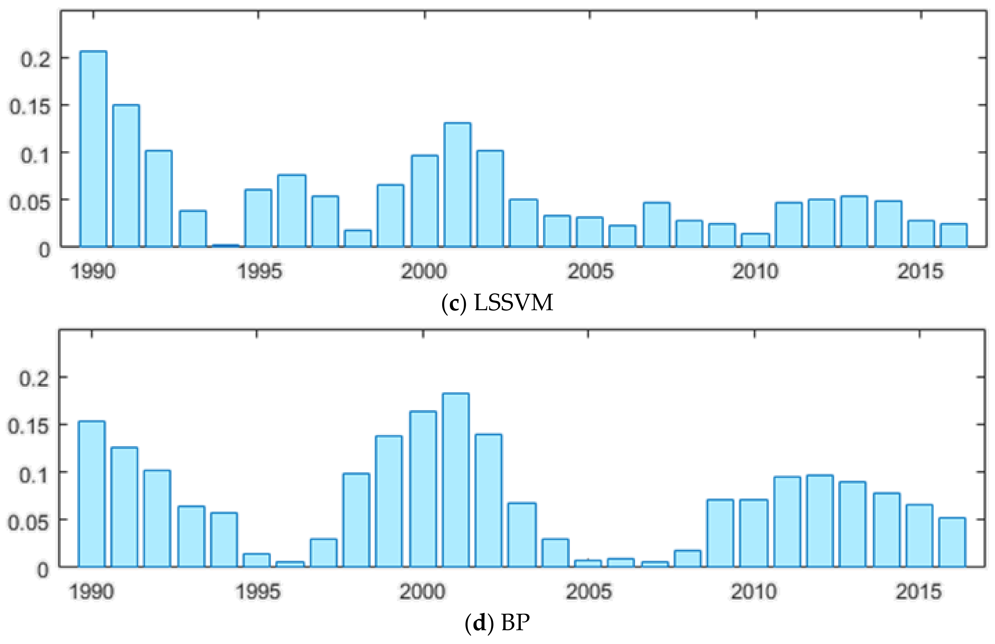
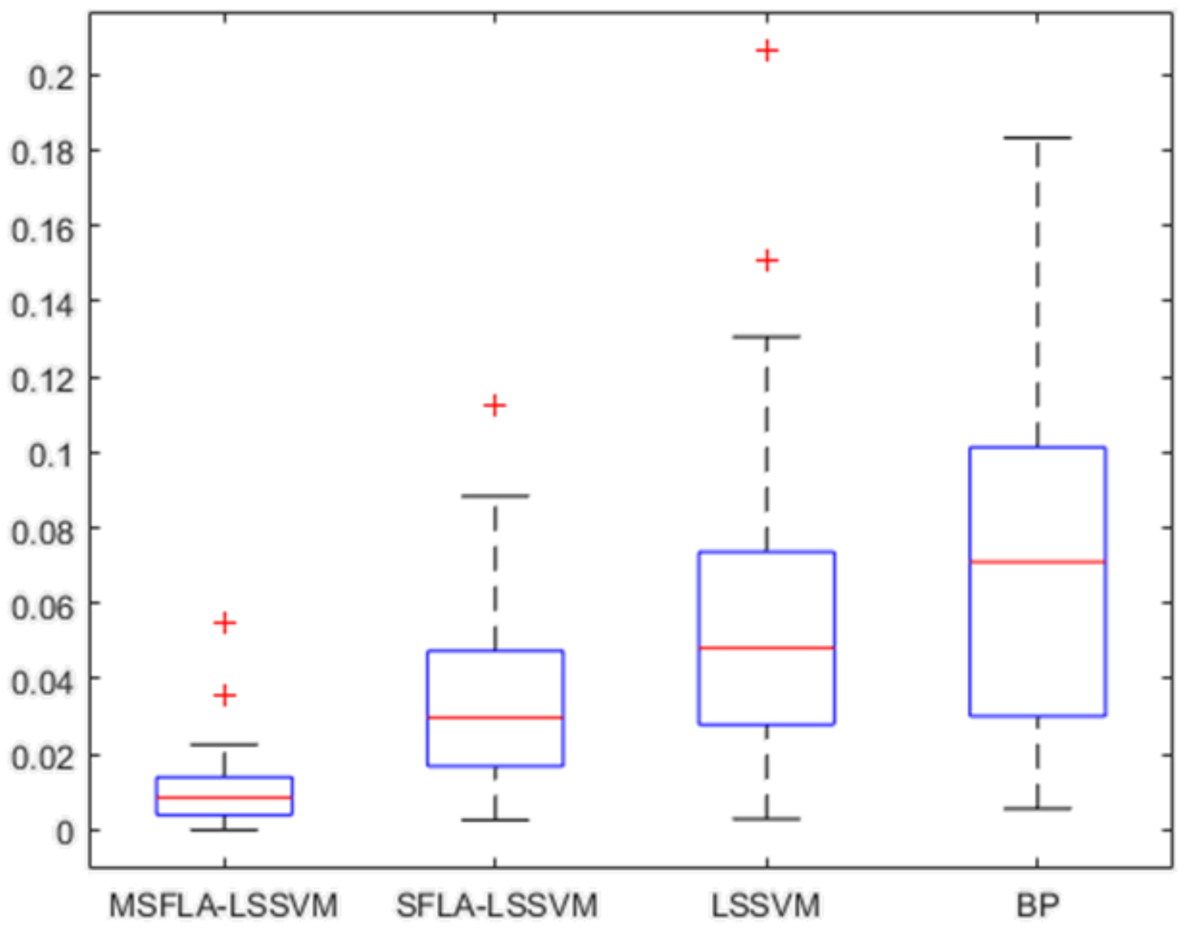
3.2. Forecasting Effect Test for MSFLA-LSSVM Model

We take the data from 1990 to 2009 as the training set, and the test set is the data from 2010 to 2016. The MSFLA-LSSVM model is used to forecast the CO₂ emissions. The model parameters settings are as follows: the frog population is 300; the sub-population is 30; the sub-population search number is 10; the regularization parameter search range of LSSVM is [0.1, 200] and the RBF kernel parameter is [0.01, 20]; the maximum number of iterations is 200. The forecasting results and the residuals are shown in Figure 3.

The relative error of each prediction point is shown in

Table 2. The relative error.

Year	Actual Value (100 Million Tons)	Forecasting Value (100 Million Tons)	RE (%)
1990	24.42	25.7652	5.4901
1991	25.66	26.1883	2.0751
1992	26.90	26.7878	0.4341
1993	28.79	27.7606	3.5654
1994	30.58	30.4319	0.4920
1995	33.20	33.5666	1.0954
1996	34.63	34.6415	0.0306
1997	34.70	34.0794	1.7745
1998	33.24	33.3170	0.2214
1999	33.18	33.6607	1.4469
2000	34.05	34.1477	0.2816
2001	34.88	35.1770	0.8640
2002	38.50	38.0218	1.2489
2003	45.40	45.1682	0.5197
2004	52.34	52.1643	0.3270
2005	58.97	60.3021	2.2597
2006	65.29	64.4434	1.3010
2007	70.31	70.3398	0.0452
2008	75.53	75.2229	0.4075
2009	80.01	79.6572	0.4411
2010	87.76	88.6834	1.0517
2011	97.34	97.3347	0.0007
2012	100.29	99.8869	0.3977
2013	102.58	101.3635	1.1859
2014	102.92	101.9012	0.9892
2015	101.38	102.1496	0.7591
2016	100.87	102.3212	1.4387

.

From Figure 3 and Table 2, it can be concluded that using the MSFLA-LSSVM model to forecast CO₂ emissions in China can obtain good forecasting results, and the forecasting curve has a good fitting degree with the actual curve.

In order to prove the validity and superiority of the MSFLA-LSSVM model further, three models (SFLA-LSSVM, LSSVM and BP neural network) are selected to make a comparison with the MSFLA-LSSVM model and study the prediction results of the same sample. The comparison results, the relative errors and the boxplot of relative errors are shown in Figure 4, Figure 5 and Figure 6, respectively.

Figure 4 shows the fitting degree between the CO₂ emissions curve forecasted by different models and the actual curve of CO₂ emissions. Figure 5 shows the relative errors of each model for CO₂ emission forecasting. The boxplot in Figure 6 shows the minimum, first quartile, the median, third quartile and the maximum of the relative errors in each model. From Figure 5 and Figure 6, it can be seen that the MSFLA-LSSVM model has the minimum relative error, followed by the SFLA-LSSVM model and the relative error of BP is maximum.

In order to evaluate the forecasting effect of each model more objectively, $MAPE$ (mean absolute percentage error), $RMSE$ (root mean square error) and $MAE$ (mean absolute error) are applied to compare the forecasting accuracy of each model. The calculation equations are shown as follows:

$$MAPE=\frac{1}{n}{\displaystyle \sum _{i=1}^n\left|\frac{{\widehat{y}}_i-y_i}{y_i}\right|}.$$

(27)

$$RMSE=\sqrt{\frac{1}{n}{\displaystyle \sum _{i=1}^n{({\widehat{y}}_i-y_i)}^2}}.$$

(28)

$$MAE=\frac{1}{n}{\displaystyle \sum _{i=1}^n\left|{\widehat{y}}_i-y_i\right|}.$$

(29)

where ${\widehat{y}}_i$ is the predicted value; $y_i$ is the actual value; $n$ is the sample size.

The calculation results of $MAPE$, $RMSE$ and $MAE$ for different models are shown in

Table 3. The calculation results.

Model	MAPE (%)	RMSE (100 Million Tons)	MAE (100 Million Tons)
MSFLA-LSSVM	1.1165	0.7013	0.5425
SFLA-LSSVM	3.7209	2.1616	1.8467
LSSVM	5.9740	3.1515	2.8041
BP	7.5416	4.9479	3.9981

.

From Table 2, it can be concluded that $MAPE$, $RMSE$ and $MAE$ of the MSFLA-LSSVM model is the smallest in all models, reaching 1.1165%, 0.7013, and 0.5425, respectively. Next is the SFLA-LSSVM model, the $MAPE$, $RMSE$ and $MAE$ are 3.7209%, 2.1616, and 1.8467, respectively. The $MAPE$, $RMSE$ and $MAE$ of BP model is the largest, reaching 7.5416%, 4.9479, and 3.9981 respectively. Besides this, the LSSVM model has a better forecasting effect than the BP model. In a word, the evaluation results of three indexes for four models are basically the same. And the prediction accuracy is ranked as follows: MSFLA-LSSVM > SFLA-LSSVM > LSSVM>BP. It can be concluded that the forecasting accuracy of MSFLA-LSSVM model is obviously higher than that of other models, and it is effective and practical for CO₂ emissions forecasting.

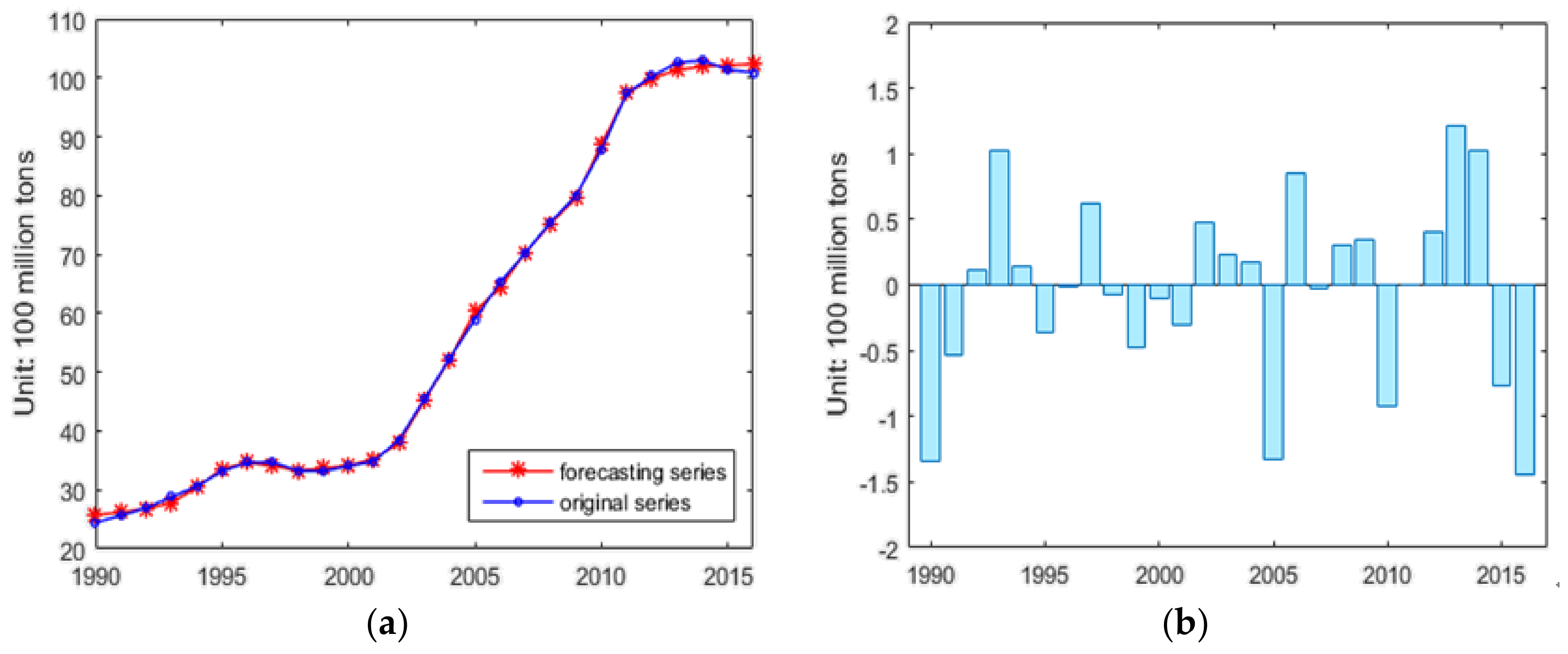
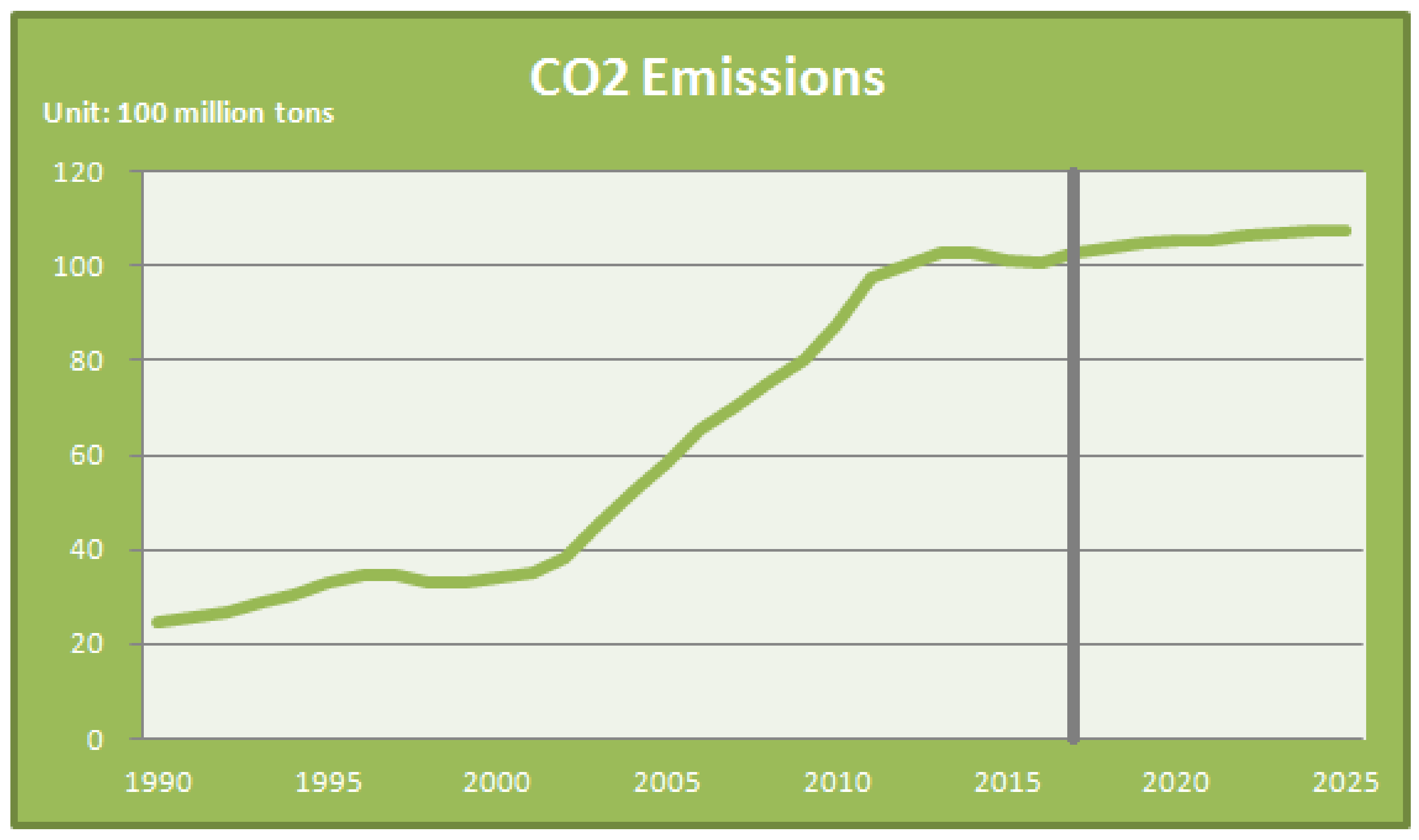
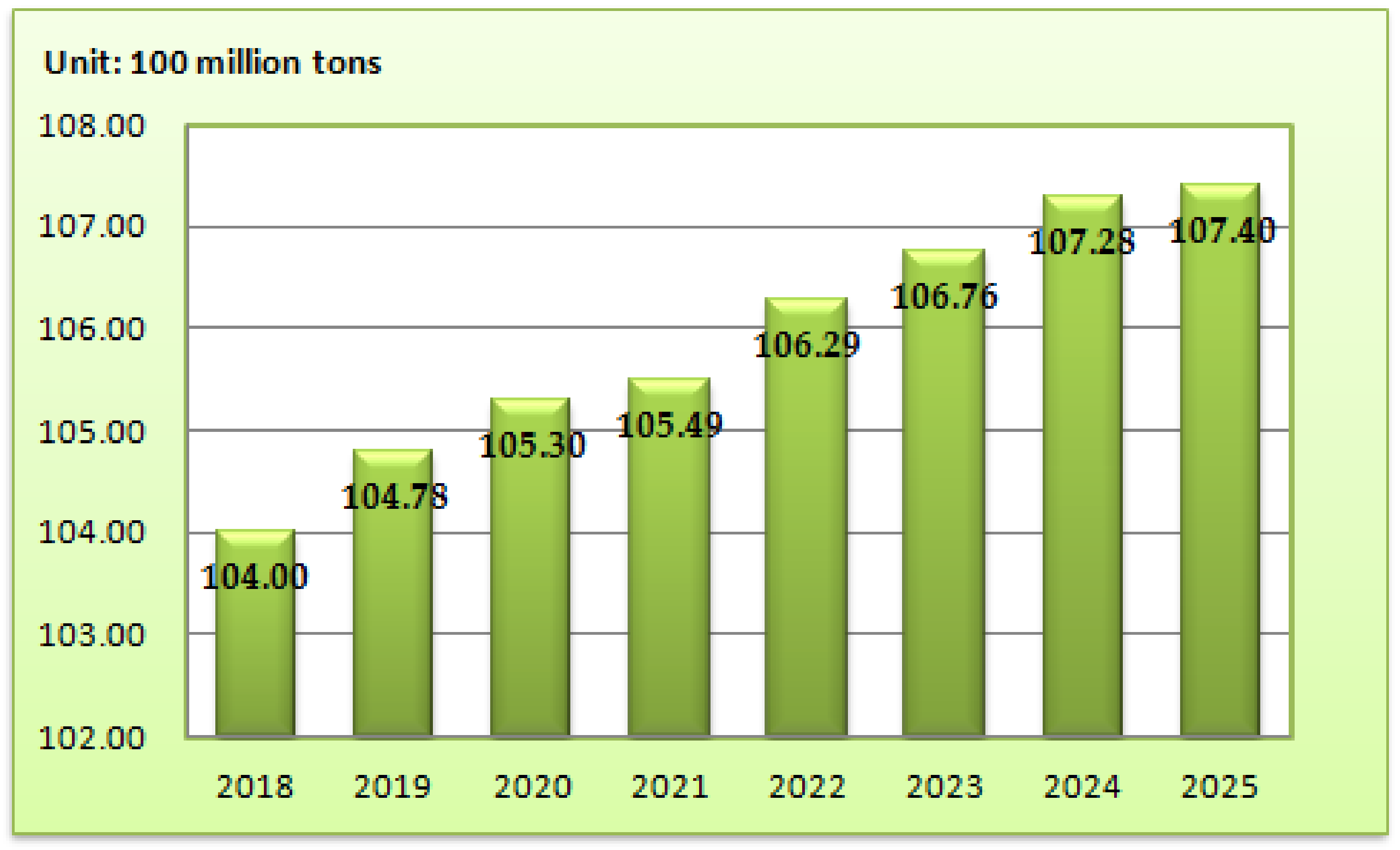
3.3. CO₂ Emissions Forecasting Based on GM(1,1) and MSFLA-LSSVM Model

Based on the collected historical data, we use GM(1,1) model to forecast CO₂ emissions influencing factors of per capita GDP, urbanization rate, total coal consumption and total imports and exports from 2018 to 2025 in China. Since the GM(1,1) model has a higher forecasting accuracy for small samples, we choose the data from 2010 to 2016 as the forecasting sample instead of the entirety of the data.

Before using the GM(1,1) model, we first do the dimensionless processing of the original data according to the Equation (30).

$$y_i=\frac{x_i-\min (x_i)}{\max (x_i)-\min (x_i)}.$$

(30)

Then, the GM(1,1) model is applied to forecast the per capita GDP, urbanization rate, total coal consumption and total imports and exports from 2018 to 2025 in China. The forecasting results are shown in Figure 7.

The predicted data above are used as the MSFLA-LSSVM model input to forecast the CO₂ emissions from 2018 to 2025 in China. The specific forecasting results are shown in Figure 8 and Figure 9.

As you can see in Figure 8 and Figure 9, China’s CO₂ emissions from 2018 to 2025 will take on a slow growth trend. China’s CO₂ emissions increased rapidly from 2002 to 2012. However, after 2012, the CO₂ emissions grew slowly and got into the platform period. With the strengthening of the policies on CO₂ emissions reduction in China, it is foreseeable that CO₂ emissions will be effectively controlled and the greenhouse effect will be relieved in the future.

4. Conclusions

In order to forecast CO₂ emissions in China accurately, considering population, the CO₂ emission forecasting model using GM(1,1) and LSSVM optimized by MSFLA (MSFLA-LSSVM) is put forward in this paper. First of all, considering population, per capita GDP, urbanization rate, industrial structure, energy consumption structure, energy intensity, total coal consumption, carbon emissions intensity, total imports and exports and other influencing factors of CO₂ emissions, the main driving factors are screened according to the sorting of grey correlation degrees to realize feature dimension reduction. Then, the GM(1,1) model is used to forecast the main influencing factors of CO₂ emissions. Finally, taking the forecasting value of the CO₂ emissions influencing factors as the model input, the MSFLA-LSSVM model is adopted to forecast the CO₂ emissions in China from 2018 to 2025.

According to the forecasting results of the CO₂ emissions from 2018 to 2025 in China, it can be seen that China’s CO₂ emissions will take on a slow growth trend in the next few years. With the strengthening of the policy on CO₂ emissions reduction in China, China’s CO₂ emissions will be effectively controlled in the future, and then the greenhouse effect will be relieved.

References

1. Safdarnejad, S.M.; Hedengren, J.D.; Baxter, L.L. Plant-level dynamic optimization of Cryogenic Carbon Capture with conventional and renewable power sources. Appl. Energy 2015, 149, 354–366. [Google Scholar] [CrossRef]
2. Safdarnejad, S.M.; Hedengren, J.D.; Baxter, L.L. Dynamic optimization of a hybrid system of energy-storing cryogenic carbon capture and a baseline power generation unit. Appl. Energy 2016, 172, 66–79. [Google Scholar] [CrossRef]
3. Gopan, A.; Kumfer, B.M.; Phillips, J.; Thimsen, D.; Smith, R.; Axelbaum, R.L. Process design and performance analysis of a Staged, Pressurized Oxy-Combustion (SPOC) power plant for carbon capture. Appl. Energy 2014, 125, 179–188. [Google Scholar] [CrossRef]
4. Cohen, S.M.; Rochelle, G.T.; Webber, M.E. Optimizing post-combustion CO2, capture in response to volatile electricity prices. Int. J. Greenh. Gas Control 2012, 8, 180–195. [Google Scholar] [CrossRef]
5. Ismail, Z.; Yahaya, A.; Shabri, A. Forecasting Gold Prices Using Multiple Linear Regression Method. Am. J. Appl. Sci. 2009, 6, 1509–1514. [Google Scholar] [CrossRef]
6. Liu, D.; Bai, X.; Meng, J. Multiple linear regression forecasting model of total food yield in China based on forward selection variables method. J. Northeast Agric. Univ. 2010, 41, 24–128. [Google Scholar]
7. Sehgal, V.; Tiwari, M.K.; Chatterjee, C. Wavelet Bootstrap Multiple Linear Regression Based Hybrid Modeling for Daily River Discharge Forecasting. Water Resour. Manag. 2014, 28, 2793–2811. [Google Scholar] [CrossRef]
8. Ming, Z.; Liu, D.; Kaiyan, D.; Song, X.; Yulong, L.; Haiyan, Z. Pre-integrated Forecasting Method Research of Urban Electricity Consumption Based on System Dynamics and Econometric Model. J. Appl. Sci. 2013, 13, 4732–4737. [Google Scholar] [CrossRef]
9. Dyson, B.; Chang, N.B. Forecasting municipal solid waste generation in a fast-growing urban region with system dynamics modeling. Waste Manag. 2005, 25, 669–679. [Google Scholar] [CrossRef]
10. Venkatesan, A.K.; Ahmad, S.; Johnson, W.; Batista, J.R. Systems dynamic model to forecast salinity load to the Colorado River due to urbanization within the Las Vegas Valley. Sci. Total Environ. 2011, 409, 2616–2625. [Google Scholar] [CrossRef]
11. Hsu, C.C.; Chen, C.Y. Applications of improved grey prediction model for power demand forecasting. Energy Convers. Manag. 2003, 44, 2241–2249. [Google Scholar] [CrossRef]
12. Lee, Y.S.; Tong, L.I. Forecasting energy consumption using a grey model improved by incorporating genetic programming. Energy Convers. Manag. 2011, 52, 147–152. [Google Scholar] [CrossRef]
13. Matjafri, M.Z.; Lim, H.S. Prediction models for CO2 emission in Malaysia using best subsets regression and multi-linear regression. SPIE Proc. 2015, 9638, 12. [Google Scholar] [CrossRef]
14. Zhong, Q. Prediction of energy consumption and CO2 emission by system dynamics approach. Chin. J. Eco-Agric. 2008, 16, 1043–1047. [Google Scholar] [CrossRef]
15. Lin, C.S.; Liou, F.M.; Huang, C.P. Grey forecasting model for CO2 emissions: A Taiwan study. Adv. Mater. Res. 2011, 88, 3816–3820. [Google Scholar] [CrossRef]
16. Huang, D.Z.; Gong, R.X.; Gong, S. Prediction of Wind Power by Chaos and BP Artificial Neural Networks Approach Based on Genetic Algorithm. J. Electr. Eng. Technol. 2015, 10, 41–46. [Google Scholar] [CrossRef]
17. Bin, H.; Zu, Y.X.; Zhang, C. A Forecasting Method of Short-Term Electric Power Load Based on BP Neural Network. Appl. Mech. Mater. 2014, 538, 247–250. [Google Scholar] [CrossRef]
18. Narayanakumar, S.; Raja, K. A BP Artificial Neural Network Model for Earthquake Magnitude Prediction in Himalayas, India. Circuits Syst. 2016, 7, 3456–3468. [Google Scholar] [CrossRef]
19. Yang, J.F.; Cheng, H.Z. Application of SVM to power system short-term load forecast. Electr. Power Autom. Equip. 2004, 24, 30–32. [Google Scholar]
20. Hong, W.C. Electric load forecasting by support vector model. Appl. Math. Model. 2009, 33, 2444–2454. [Google Scholar] [CrossRef]
21. Gallo, C.; Contò, F.; Fiore, M. A Neural Network Model for Forecasting CO2 Emission. AGRIS Econ. Inform. 2014, 6, 31. [Google Scholar]
22. Zhou, J.G.; Zhang, X.G. Projections about Chinese CO2 emissions based on rough sets and gray support vector machine. China Environ. Sci. 2013, 33, 2157–2163. [Google Scholar]
23. De Giorgi, M.G.; Malvoni, M.; Congedo, P.M. Comparison of strategies for multi-step ahead photovoltaic power forecasting models based on hybrid group method of data handling networks and least square support vector machine. Energy 2016, 107, 360–373. [Google Scholar] [CrossRef]
24. Li, X.; Wang, X.; Zheng, Y.H.; Li, L.X.; Zhou, L.D.; Sheng, X.K. Short-Term Wind Power Forecasting Based on Least-Square Support Vector Machine (LSSVM). Appl. Mech. Mater. 2013, 448, 1825–1828. [Google Scholar] [CrossRef]
25. Zhao, H.; Guo, S.; Zhao, H. Energy-Related CO2 Emissions Forecasting Using an Improved LSSVM Model Optimized by Whale Optimization Algorithm. Energies 2017, 10, 874. [Google Scholar] [CrossRef]
26. Yang, W.; Li, Q. Survey on Particle Swarm Optimization Algorithm. Eng. Sci. 2004, 6, 87–94. [Google Scholar]
27. Trelea, I.C. The particle swarm optimization algorithm: Convergence analysis and parameter selection. Inform. Process. Lett. 2016, 85, 317–325. [Google Scholar] [CrossRef]
28. Zwickl, D.J. Genetic algorithm approaches for the phylogenetic analysis of large biological sequence datasets under the maximum likelihood criterion. Diss. Theses Gradworks 2006, 3, 257–260. [Google Scholar]
29. Deb, K. An efficient constraint handling method for genetic algorithms. Comput. Meth. Appl. Mech. Eng. 2000, 186, 311–338. [Google Scholar] [CrossRef]
30. Karaboga, D.; Basturk, B. A powerful and efficient algorithm for numerical function optimization: Artificial bee colony (ABC) algorithm. J. Glob. Optim. 2007, 39, 459–471. [Google Scholar] [CrossRef]
31. Karaboga, D.; Basturk, B. On the performance of artificial bee colony (ABC) algorithm. Appl. Soft Comput. 2008, 8, 687–697. [Google Scholar] [CrossRef]
32. Akay, B.; Karaboga, D. A modified Artificial Bee Colony algorithm for real-parameter optimization. Inform. Sciences 2012, 192, 120–142. [Google Scholar] [CrossRef]
33. Wang, B.Y.; Wang, D.Y.; Zhang, S.M. A Short-Term Distributed Load Forecasting Algorithm Based on Spark and IPPSO_LSSVM. Appl. Mech. Mater. 2015, 713–715, 1385–1388. [Google Scholar]
34. Wen, T.; Tang, H.; Wang, Y.; Lin, C.Y.; Xiong, C.R. Landslide displacement prediction using the GA-LSSVM model and time series analysis: A case study of Three Gorges Reservoir, China. Nat. Hazard Earth Syst. Sci. 2017, 17, 2181–2198. [Google Scholar] [CrossRef]
35. Mustaffa, Z.; Yusof, Y. Optimizing LSSVM using ABC for non-volatile financial prediction. Aust. J. Basic Appl. Sci. 2011, 7, 549. [Google Scholar]
36. Eusuff, M.M.; Lansey, K.E. Optimization of Water Distribution Network Design Using the Shuffled Frog Leaping Algorithm. J. Water Resour. Plan. Manag. 2003, 129, 210–225. [Google Scholar] [CrossRef]
37. Eusuff, M.; Lansey, K.; Pasha, F. Shuffled frog-leaping algorithm: A memetic meta-heuristic for discrete optimization. Eng. Optim. 2006, 38, 129–154. [Google Scholar] [CrossRef]
38. Zhao, Z.; Xu, Q.; Jia, M. Improved shuffled frog leaping algorithm-based BP neural network and its application in bearing early fault diagnosis. Neural Comput. Appl. 2016, 27, 375–385. [Google Scholar] [CrossRef]
39. Pan, Q.K.; Wang, L.; Gao, L.; Li, J. An effective shuffled frog-leaping algorithm for lot-streaming flow shop scheduling problem. Int. J. Adv. Manuf. Technol. 2011, 52, 699–713. [Google Scholar] [CrossRef]
Figure 1. The flow of the forecasting model.
Sustainability 10 00958 g001
Figure 2. The sample data of the CO2 emissions and the selected influencing factors.
Sustainability 10 00958 g002
Figure 3. The forecasting result and residual error.
Sustainability 10 00958 g003
Figure 4. Comparison of forecasting results.
Sustainability 10 00958 g004
Figure 5. The relative errors of four models: (a) modified shuffled frog leaping algorithm (MSFLA)–least squares support vector machine (LSSVM); (b) shuffled frog leaping algorithm (SFLA)-LSSVM; (c) LSSVM; (d) BP (back propagation).
Sustainability 10 00958 g005aSustainability 10 00958 g005b
Figure 6. The boxplot for four models.
Sustainability 10 00958 g006
Figure 7. The forecasting results of per capita GDP, urbanization rate, total coal consumption and total imports and exports.
Sustainability 10 00958 g007
Figure 8. The forecasting results of CO2 emissions.
Sustainability 10 00958 g008
Figure 9. The forecasting results of CO2 emissions from 2018 to 2025 in China.
Sustainability 10 00958 g009