Spatial Spillover Effects of Environmental Pollution in China’s Central Plains Urban Agglomeration


1
School of Economics and Management, Beijing Forestry University, Beijing 100083, China
2
Faculty of Technology, Policy & Management, Delft University of Technology, Mekelweg 2, 2628 CD Delft, The Netherlands
3
School of International Relations and Public Affairs, Fudan University, Shanghai 200433, China
4
College of Economics and Management, China Agricultural University, Beijing 100083, China
*
Authors to whom correspondence should be addressed.
Sustainability 2018, 10(4), 994; https://doi.org/10.3390/su10040994
Submission received: 8 February 2018
/
Revised: 21 March 2018
/
Accepted: 26 March 2018
/
Published: 28 March 2018
(This article belongs to the Section Economic and Business Aspects of Sustainability)
Abstract
:Promoting the rise of Central China is one of the most important national strategies regarding the promotion of China’s economic development. However, the environmental issues in the central regions have become remarkably severe. It is therefore worthwhile exploring how economic development and environmental protection can be coordinated. Focusing on the 29 prefecture-level cities in the Central Plains Urban Agglomeration, the authors empirically analyze the relationship between the economy and the environment from 2004 to 2014. The combined methods of the spatial autocorrelation model, the environmental Kuznets curve, and the global spatial correlation test are systematically employed. The results show that: (1) a strong spatial correlation exists between industrial wastewater discharge, industrial sulfur dioxide, and dust emissions in the Central Plains Urban Agglomeration; (2) the relationship between the economy and the environment of this urban agglomeration reveals an inverted “U” curve, which confirms the classical environmental Kuznets curve hypothesis. Industrial dust emissions have surpassed the inflection point of the Kuznets curve, but its spatial spillover effect still remains strong. This is caused by an accumulation effect and a lag effect; (3) the proportion of the secondary industry and population has a strong positive effect on pollution discharge; investments in science and technology have a certain inhibitory effect on industrial sulfur dioxide emission. Moreover, an increase in the number of industrial enterprises has a negative effect on industrial wastewater emission. At the end, the authors put forward policy recommendations regarding the establishment of a joint supervisory department and unified environmental standards at the regional level to deal with the spillover effects of pollution.
1. Introduction
In 2016, China’s State Council approved the Development Plan for Central Plains Urban Agglomeration. Since then, Central Plains Urban Agglomeration (CPUA) has been officially enacted as a national-level urban agglomeration. According to the document, the Development Plan for the CPUA issued by the National Development and Reform Commission in December 2016, the CPUA is located in Central China, covering 30 prefecture-level cities in the provinces Henan, Shanxi, Hebei, Shandong, and Anhui (Figure 1). It has a total area of 287,000 km2 and an urbanization rate of about 50%. By the end of 2016, the CPUA had 158 million people and a per capita GDP of 3.51 million Yuan. Its GDP reached 5.56 trillion Yuan, ranking the fourth among China’s urban agglomerations, immediately behind Yangtze River Delta, Pearl River Delta, and Beijing–Tianjin–Hebei region. The central plains refers to the middle and lower reaches of the Yellow River, including the most parts of Henan Province, the southern part of Hebei Province, the southern part of Shanxi Province, the east of Shaanxi province, and the west of Shandong province. The CPUA is part of the central plains. As one of the most important economic growth poles, the CPUA is significant in boosting the rise of Central China and spreading economic development further to the central–western regions.
However, the price of rapid economic growth is environmental degradation and higher energy consumption. As an important industrial base in the central regions, the CPUA’s secondary industry accounts for over 50%, of which heavy industry is the main component. By the end of 2014, the “three industrial wastes” (i.e., industrial wastewater, industrial sulfur dioxide (SO2), and industrial dust) in the CPUA had reached 2019.28 million tons, including 2016.28 million tons of industrial wastewater, 1.6 million tons of industrial SO2, and 1.4 million tons of industrial dust. The wastewater and industrial SO2 are mainly emitted by the steel, coal, and manufacturing industries. The construction industry and mining industry generate the vast majority of the industrial dust. Consequently, the environmental problems in the CPUA are extremely serious [1]. As experience in the developed countries and regions tells, economic growth and environmental pollution generally have an inverted U-shaped relationship, which is also known as the environmental Kuznets curve (EKC) [2,3]. As economic growth rises, the physical environment begins to deteriorate. However, after the economy reaches a certain level, the pollution levels will gradually taper off or even decline, which is called “Pollution First, Treatment Later” [4]. The authors wonder whether the CPUA shows similar features in its development process. If so, it is important to recognize the patterns of industrialization and urbanization for developing customized regional policies.
There have been plentiful studies about the CPUA’s sustainable development, because the region plays a significant role in driving the economy of Central China as a whole. It determines whether the strategy of rising Central China can progress significantly [5,6]. Qiu et al. (2014) measured the CPUA’s level of development in terms of employment, industrial development, and land use. Their results have shown that the rapid population growth and industrial development were mainly derived from the secondary sector, while the tertiary industry remained relatively backward. Regarding its industrial structure, Feng and Han [7] have found that the proportion of the CPUA’s secondary industry in the total economy was higher than the national average (46.8%), and the proportion of its tertiary industry was far lower than the national average (43.1%). In sum, its industrial structure is open to being optimized. The gap in development among various cities in the CPUA is large. Tong et al. [8] provided evidence that due to urbanization and industrialization, biodiversity is under threat, and air and water pollution have worsened. Furthermore, Miao et al. [9] have analyzed the emergence of the CPUA, and discussed how the urban agglomeration and urban spatial network can be defined. They found that the urban agglomeration was not only a complex urban area system with multiple cities as its core, but also a high-density integrated network between towns. From the perspective of the coordinated development, Cui and Wang et al. [10,11] found that urbanization and ecological deterioration were not well coordinated across the CPUA region. In terms of the spatial linkages between cities in the CPUA, based on microblogging data, Wang and Deng [3] found that these linkages had a circle-layer character and a spatial imbalance. Three levels of spatial connection could be identified according to the size and the distance of these cities. All of these studies have given rise to concerns regarding the CPUA’s sustainable development, mainly due to its vital position in Central China’s economy and ecology. However, most of the literature uses either an industrial economics or an urban planning perspective. There has been little research on the spillover effects of pollution through spatial econometrics to integrate environmental, economic, and urbanization insights.
The goal of this contribution is to detect the spillover effects of the CPUA’s coordinated development in terms of economic growth and environmental deterioration. Besides, further analysis is conducted to uncover whether the CPUA reveals a typical EKC pattern. Research findings will shed light on synchronizing the development of the CPUA’s industrialization, urbanization, and environmental protection. The outline of this article is as follows. Section 2 reviews EKC theory in connection with regional development, and introduces the procedure that is used for collecting data and selecting variables. The application of EKC theory in spatial econometric models is demonstrated in Section 3. Section 4 presents the status quo of the CPUA’s environmental performance based on spatial distribution. Subsequently, our empirical results are presented based on the EKC and spatial autocorrelation (SAC) model. Section 5 discusses the obtained empirical results based on policy analysis. Conclusions are drawn, and policy recommendations are provided in Section 6.
2. Research Methodology and Data Collection
2.1. Environmental Kuznets Curve with Spatial Econometrics
The environmental Kuznets curve (EKC) is a key theory in connecting the environment and the economy. Its main point is that environmental quality will deteriorate in the early stages of economic development, but when the economic development reaches a certain level, it will improve after a while [4,12]. For example, some scholars use the EKC to study whether economic growth improves environmental quality [13]. Apergis and Ozturk [14] have examined the relationship between CO2 emissions and economic development in 14 Asian countries. They concluded that there was an inverted U-shaped relationship in line with the EKC theory. Regarding the applicability of the EKC to China, a series of empirical tests is required to analyze whether China’s economy and environment are consistent with the EKC hypothesis. This is due to the specific features of China’s economic models and resource consumption structure. For example, Brajer et al. [15] used China’s urban panel data to verify the relationship between economic growth and SO2 pollution. The results confirmed the existence of the EKC hypothesis in China, and found that technological progress was an important factor to mitigate environmental pollution. Yu-Ming et al. [16] used cross-sectional data of China’s 31 provinces to analyze the spatial correlation of provincial pollution through a spatial metrology model. Their results showed that three spatial dependence and spatial spillover effects were obvious in China’s provincial environmental pollution. Hao et al. [17] used provincial panel data and a spatial econometric model to analyze the EKC in terms of China’s energy and electricity consumption curve. They found that China’s energy and electricity consumption and per capita gross domestic product (GDP) presented an inverted N-type EKC. Ertugrul et al. [18] studied the relationship between per capita income and energy consumption in the major developing countries. The results showed that the EKC hypothesis applied best to the countries with fast economic growth, such as China. Dong et al. [19] used the panel data of 30 provinces in China from 1995~2014 to study the validity of the EKC hypothesis in CO2 emissions. The results showed that the EKC hypothesis can be verified in China’s central and eastern regions. They concluded that CO2 emissions were not related to the level of economic development, but were related to the regional energy consumption structure.
Moreover, many scholars have added a variety of control variables to empirical analyses of the relationship between economic growth and environmental pollution, such as industrial structure, foreign trade values, population size, energy consumption, research and development investments, and urbanization rates. Empirical tests with diverse variables can accurately reflect how the major factors influence environmental performance [14,20,21,22,23,24,25,26]. From the existing literature, one can learn that the combination of spatial econometrics and the EKC theory is growing increasingly popular for analyzing the dynamic relationship between the regional economy and environmental performance. Moreover, the spatial relationship among the cities in one urban agglomeration deserves more attention. Therefore, this paper will pair the EKC theory with spatial measurement methods to test the spatial spillover effects of the CPUA’s environmental pollution.
2.2. Data Collection and Variable Description
The research data are the panel data of 29 prefecture-level cities in the CPUA from 2004 to 2014, which were acquired from the China Urban Statistical Yearbook, China Environmental Statistical Yearbook, Statistical Yearbook of Henan Province, Statistical Yearbook of Shanxi Province, Statistical Yearbook of Hebei Province, Statistical Yearbook of Shandong Province, and Statistical Yearbook of Anhui Province. The original CPUA includes 30 prefecture-level cities in accordance with the document the Development Plan of the CPUA issued by the National Development and Reform Commission. Due to the lack of relevant data of Jiyuan city, we select the other 29 prefecture-level cities as sample areas.
Based on the literature and our previous work [25], we have selected per capita GDP as the independent variable to reflect economic growth, and three dependent variables in terms of environmental performance. Table 1 summarizes the descriptions of the variables. Environmental pollution is mainly emitted through industrial activities [26,27]; the authors have therefore selected the industrial wastewater discharge, industrial SO2 emission, and industrial dust emission levels of 29 prefecture-level cities in the CPUA. These pollution indices, especially the air pollution, are the representative hazardous emissions in the CPUA region due to coal mining and steel production. Currently, the CPUA is suffering from severe air pollution (PM 2.5), especially from SO2 and industrial dust. Furthermore, in order to improve the rigor of this research, five control variables have been selected, including: (1) the proportion of the secondary industry in GDP, (2) population size, (3) foreign investment volume, (4) investment in science and technology, and (5) the number of industrial enterprises with a designated size or above (according to the definition of the China National Bureau of Statistics, the industrial enterprises with a designated size or above refers to the industrial enterprises with an annual main business income of more than 20 million Yuan).
The proportion of the secondary industry in the GDP represents the scale and degree of industrial development. If this proportion is higher, in theory, the emission levels of industrial pollution are higher [22,28]. Moreover, the larger the population is, the greater the pressure on the physical environment, which is harmful to the ecological balance [21,24]. A larger scale of foreign capital investment in a region may indicate a higher level of openness in regions. Rapid industrial expansion will generate a corresponding increase in energy consumption [14,29]. In fact, the energy consumption in the CPUA region is mainly caused by coal burning, which generates high levels of industrial SO2 and dust. Technological investment represents the level of regional science and technology [15,18]. The higher the technological investment, the more effective the production mode. The number of industrial enterprises with a designated size or above can influence energy consumption. If this number is larger, it implies that the energy consumption increases, which generates more pollution [30,31]. In addition, Table 1 also demonstrates the expected direction and impact of the independent variables and control variables.
3. Application of the EKC Theory with Spatial Econometric Models
3.1. EKC Model
The traditional EKC hypothesis refers to the existence of a quadratic curve between economic growth and environmental pollution, and its benchmark model is:
In Equation (1), α0 is the constant term; β is the parameter to be estimated; ε is the random disturbance term; i is the city; and t is the year. Y is the environmental pollution index, including: industrial wastewater discharge, industrial SO2 emissions, and industrial dust emissions. The higher the Y value, the more serious the environmental pollution. As to the rigorous econometric model, multiple terms of explanatory variables in the EKC model will lead to a higher probability of serious multicollinearity in its variables, which is not conducive to the accuracy of the results [32]. Therefore, this research follows the relatively mature approach [33,34,35], assuming that economic growth has a quadratic relationship with environmental pollution in the CPUA, bringing the control variables into the model as follows:
In Equation (2), C is the control variable; and η is the parameter to be estimated. Control variables mainly include: industrial structure, population size, the scale of foreign direct investment, investment in science and technology, and the number of industrial enterprises with a designated size or above. Additionally, the logarithmic processing on both sides of the equation allows the avoidance of serious fluctuations in the data without affecting their original features. It also eliminates possible heteroscedasticity [36]. Therefore, the authors eventually use the following logarithmic EKC model:
Table 2 lists the evaluation criteria for the quadratic curve (curve-shaped) relating economic development with environmental pollution, which uses regression coefficient characteristics to determine the relationship. The criteria are mainly based on the existing EKC literature.
3.2. Moran Index and Spatial Autocorrelation (SAC) Model
Most studies on economic growth and environmental pollution do not take into account the spatial correlation with environmental pollution. However, if the spatial characteristics of environmental pollution are neglected, regression results will be biased [37]. To this end, the Moran index is tested to discover the spatial correlation between 29 cities in the CPUA [38,39]. The “global Moran index I” is used to test the global spatial autocorrelation. The equation reads as follows:
In Equation (4), wij is the (i, j) factor of the spatial weight matrix, which is used to measure the distance between region i and region j. If region i and region j are adjacent, we set wij = 1, otherwise wij = 0. is the sum of all the spatial weights. The values of Moran’s I are generally between −1 and 1. If the value is greater than 0 and close to 1, a positive correlation is observed. In contrast, if the value is less than 0 and close to −1, we see a negative correlation. Based on the theory of spatial econometrics developed by Lesage and Pace [40], we propose the following spatial measurement model:
Equation (5) is the spatial econometric benchmark model of panel data. In this equation, is the i row of the spatial weight of matrix W: . means the individual effect of region i. is a spatial lag term. The model will be a standard static panel model if is not considered. is the spatial autocorrelation coefficient of the explanatory variables, which reflects the degree of influence of the residual term in adjacent regions on the residual term in this region. Next, the EKC model and the spatial autocorrelation model are combined as Equations (6) and (7), in order to analyze the pattern of the economic growth and environmental pollution in the CPUA:
In Equation (6), is the spatial lag term of the explanatory variables; is the time effect; λ is the spatial autocorrelation coefficient of the explanatory variables, which reflects the degree of influence of the residual term of adjacent regions on the residual term of this region. If the panel data constitutes a static panel, . In Equation (7), is the i row of the spatial weight of the disturbance term; and represents the perturbation term and error term that follows the normal distribution. In general, the common spatial econometric model includes spatial lag model (SLM) and spatial error model (SEM). The main difference between these two models is the form of spatial autocorrelation inserted into the equation [41]. In addition, there are the spatial Durbin model (SDM) and the spatial autocorrelation model (SAC). Selecting which model depends on the following circumstances: (1) if , the model will be SDM; (2) if and , the model will be SAR; (3) if and , the model will be SAC; (4) if and , the model will be SEM.
4. Results
4.1. The Status Quo of the CPUA’s Environmental Performance Based on Spatial Distribution
Preliminary research into the status quo of the CPUA’s economic development and environmental performance was conducted through spatial analysis using Acrmap Software 10.0. Figure 2 shows the spatial distribution graphs based on the annual data from 2004 to 2014 regarding industrial wastewater discharge, industrial SO2 emissions, industrial dust emissions, and per capita GDP. Five features can be observed. (1) The distribution of three types of pollutants is concentrated in the CPUA’s northern and central–western regions. The per capita GDP has a similar spatial distribution as the pollutants. The northern and central–western regions have a relatively higher per capita GDP than the southeastern region. Having similar patterns of pollution and per capita GDP implies a possible spatial link that will be tested in the later analysis; (2) In terms of industrial wastewater, the large discharge areas are mainly concentrated in the CPUA’s middle and the northern regions. Liaocheng City (in Shandong Province), Jiaozuo City, Xinxiang City, and Zhengzhou City (all three in Henan Province) produce the highest wastewater emissions, with average annual emission levels of over 90 million tons. The cities with emissions less than 50 million tons are mainly concentrated in the CPUA’s southeastern and western regions; (3) Regarding industrial SO2 emissions, Handan City in Hebei Province and Luoyang City in Henan Province produce relatively high emission levels, with average annual emissions of more than 133,000 tons. Notably, the central–western and northern regions have significantly higher SO2 emissions than the eastern and southern regions; (4) The distribution of industrial dust shows that the most polluting cities are Handan City and Changzhi City (in Shanxi Province), with average annual emissions of more than 86,000 tons. The two cities are adjacent, possibly generating a certain spatial effect on their dust pollution. The dust pollution in the eastern, central, and southern regions is relatively limited; (5) As to the economic development, Zhengzhou City, Jiaozuo City, Luoyang City, and Sanmenxia City (all three in Henan Province) have the highest level of economic development. Their annual per capita GDP is over 29,000 Yuan. The per capita GDP of southeastern cities, on the other hand, is relatively low. To summarize, we find that economic development and environmental pollution in the CPUA may well be positively correlated. We will further verify this though the econometric models in the following sections.
4.2. Model Applicability Test
First, the variance inflation factor (VIF) is introduced to observe whether the explanatory variables show serious multicollinearity. The results in Table 3 show that the maximum value of VIF does not exceed 10, and the minimum is not below 0. It demonstrates that there is no serious multicollinearity problem in the explanatory variables.
Second, Global Moran’s I is calculated to test whether any spatial autocorrelation exists in the CPUA. The results in Table 4 show that except for a few parts of the year or the index, the Moran’s I value of three types of environmental pollutants all strongly reject the original hypothesis of “no spatial autocorrelation”. This indicates that the spatial autocorrelation does exist. Therefore, we use the spatial econometric model to further analyze how the correlation behaves in the CPUA’s economic and environmental developments.
In addition, we assume that the model adapts to any of the four spatial models of SDM, SAR, SAC, and SEM, and then take the model’s suitability test. We use the Wald test and likelihood ratio (Lratio) to test the spatial autocorrelation coefficient of the explained variables (ρ) and the spatial autocorrelation coefficient of the explanatory variables (λ) (Federico et al., 2016). The results are summarized in Table 5. The Wald test (p = 0.0025 < 0.05) and the Lratio test (p = 0.0002 < 0.05) reject the original hypothesis of respectively, which excludes the SDM, SAR, and SEM models. Plus, this model is a static panel model, and . Consequently, the SAC model is selected to conduct the regression analysis.
Finally, to determine whether using a fixed effect or a random effect, the Hausman test is used for the panel data. The test results show that the p value is lower than the original hypothesis of the default value of 0.05 in STATA 13.0 software (Table 5). Thus, the original hypothesis that uses random effects can be rejected, and the fixed effect for regression estimation should be chosen.
It is important to note that until this step, the model cannot identify the developmental pattern of the economy and the environment like a regular EKC model. The reason is that the current regression equation is an EKC model to which spatial econometric analysis has been added. The explanatory variable coefficients in the equation do not directly reflect marginal changes in relation to the explained variables. In this case, the direct, indirect, and total effects estimated by the SAC model should be used to reflect the relationship between the explanatory variables and the explained variables. In other words, we need the coefficients of the total effect of the key explanatory variables to determine the shape of the curves and calculate the EKC inflection points [42].
4.3. Empirical Results
Table 5 shows the regression results of the SAC model. The table leads us to conclude the following:
- (1)
- The spatial autoregressive coefficient (rho), which is used to measure the spatial spillover effect, is obviously significant in the model of industrial dust production (p < 0.01). It indicates that there is a strong spatial spillover effect for industrial dust pollution in the CPUA. This result confirms that industrial dust is a form of regional pollution in the CPUA. By contrast, the spatial autoregressive coefficients of industrial wastewater and industrial SO2 are not significant, which indicates that the spatial spillover effects on wastewater and SO2 are not obvious.
- (2)
- The coefficient estimates of per capita GDP in the total effects reveal that the current economic growth and environmental pollution have an inverted “U” type relationship in the CPUA. This is in line with the classic EKC hypothesis. To be more specific, the emission of industrial wastewater has continued to increase along with the growth of per capita GDP. The results in Table 5 show that when the per capita GDP reaches 59,874 Yuan, its emissions begin to decline. Regarding industrial SO2, the emissions continue to increase with economic growth. When the per capita GDP grows to 22,026 Yuan, SO2 start to decline. The trend of industrial dust is similar to that of SO2, but its inflection point appears earlier. That is, when the per capita GDP reaches 15,994 Yuan, the amount of industrial dust begins to decline gradually.
- (3)
- Regarding the analysis of the control variables, the proportion of the secondary industry in the GDP has a great impact on industrial wastewater and industrial SO2 emissions (p < 0.05). The population size has a significant effect on industrial SO2 emissions (p < 0.01). Investment in science and technology has a certain negative effect on SO2 (P < 0.1), implying that the input of technology may reduce overall SO2 emissions. The increase in the number of industrial enterprises with a designated size or above has a strong negative effect on industrial wastewater discharge, contrary to what one would expect.
- (4)
- Table 5 also shows the turning point of the EKC. It can be found that in the discharge of industrial wastewater, the per capita GDP of its turning point is 59,874 yuan. Thereafter, the discharge of industrial wastewater began to decline, and the 95% confidence interval of the turning point was 58,519 yuan to 61,228 yuan. Combined with the mean value of the CPUA’s per capita GDP (20,969.47) in Table 1, the CPUA is still in the growth stage of industrial wastewater discharge. Its EKC curve is at the left end of the turning point. In terms of industrial SO2, the per capita GDP of the turning point is 22,026 yuan, and the confidence interval of the turning point is 20,671 yuan to 23,380 yuan, which indicates that the CPUA is close to the decline period of industrial SO2 emissions. Regarding the industrial dust, the per capita GDP of the turning point is 15,994 yuan, and the confidence interval of the corresponding turning point is 14,639 yuan to 17,348 yuan. It shows that the curve locates at the right end of the turning point, indicating that the CPUA is in the decline period of industrial dust emissions.
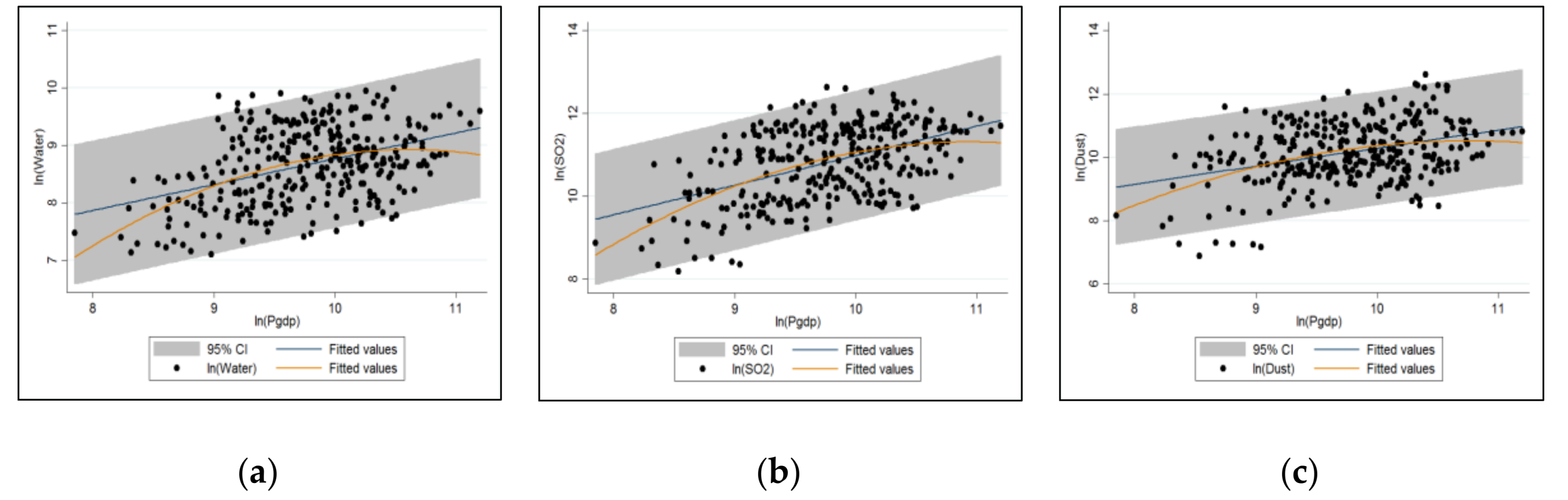
In order to intuitively reflect the relationship between industrial pollution and economic growth, we utilize quadratic fitting curves between the three types of pollutants (wastewater, SO2, and dust) and per capita GDP, and draw a 95% confidence interval. As Figure 3 demonstrates, the three curves roughly reveal an inverted “U” shape. This implies that the environment in the CPUA gradually deteriorates with economic growth, but after economic development has reached a certain level, environmental pollution would decrease. At the overall level of the CPUA, the industrial wastewater and SO2 are on the left of the turning point, meaning that these two pollutants are still going to increase for a while.
5. Discussion
Based on the preliminary analysis of the CPUA’s current environmental and economic performance, the authors found that the CPUA’s central–western areas have relatively higher pollution levels than the eastern and southern regions. This pattern matches the development of the regional per capita GDP, which indicates that there is a certain spatial relationship between the pollutant emissions and per capita GDP growth. Another preliminary finding is that the quadratic fitting curve between per capita GDP and industrial pollutants shows an inverted “U” shape. To further validate the two preliminary research findings, the SAC and EKC models have been employed to conduct empirical tests. The results of the empirical analysis confirmed that the pollution issues in the CPUA indeed have spatial spillover effects. Moreover, the CPUA’s economy and environment have revealed an inverted “U” shape curve, which is in line with the classic EKC hypothesis. Besides, the turning point of the EKC and the related 95% confidence interval indicate that the CPUA’s industrial wastewater and SO2 will increase to a certain extent. The emissions of industrial dust will decrease. In the future, the local government should strengthen the supervision of industrial wastewater and SO2 emissions.
An important finding is the spillover effects of industrial dust in the CPUA. Although the CPUA’s industrial dust emissions have surpassed the EKC inflection point along with the increase in per capita GDP, the spatial spillover effect of industrial dust pollution is still strong. In other words, industrial dust not only deteriorates the air quality in the cities where the dust originates, it also influences other areas, thus generating linkage effects for regional pollution. This phenomenon is consistent with the status quo of the air quality in the CPUA. According to the air quality monitoring data of China’s Ministry of Environmental Protection, the concentration of PM2.5 exceeded the standard (35 micrograms/cubic meter) in most areas in the CPUA in 2013. The PM2.5 of nearly two-thirds of the CPUA’s cities was higher than 70 micrograms/cubic meter (more than double the standard). Air pollution in Kaifeng and Zhengzhou was the worst. The number of the days below acceptable air quality standards accounted for 55% in 2013. Over half of the year was suffering from air pollution. However, this does not conform to the general ideas of the EKC theory. According to the EKC theory, if the CPUA’s economic development and industrial dust pollution are of an inverted “U” type and the inflection point is reached, industrial dust pollution should decrease. However, the opposite has happened. This may be related to geographic factors and atmospheric circulation speed. The CPUA’s industrial waste emissions are mainly concentrated in the western region (see Figure 2). The CPUA is located in the plains, and the west is at a higher altitude than the east. Without mountains as a shelter, air circulation rapidly spreads the dust from the west to the east, which causes the spatial spillover effect for industrial dust.
The other explanation could be the accumulation effect and lag effect of environmental pollution. The environmental pollutants are not only harmful directly after the discharge, they also continue to jeopardize the entire regional environment, even when the pollution sources are controlled. The purification capacity of the natural environment requires a certain period to clean up the pollution. The industrial dust in the CPUA has accumulated for quite a long time. Due to the limited purification capacity, the original dust pollution has not been processed, even though the total amount of dust emissions has decreased. Besides, the lack of appropriate technology also restricts the environment treatment. Thus, the accumulation effect and lag effect of dust pollution still stand out.
In terms of the control variables, the proportion of the secondary industry as a percentage of the GDP has a strong positive correlation with industrial wastewater and SO2 emissions. This is consistent with the conclusions of other scholars [22,43]. The increase of industrial wastewater and SO2 emissions will do more harm to the natural environment compared with the adverse effects of CO2 emissions on air temperature rise [44]. According to the China City Statistical Yearbook (2004–2014), the manufacturing industry is a major component of the CPUA’s industrial structure, mainly including iron and steel, metallurgy, machinery, energy, chemical, and building materials. These industries occupy over 70% of the output value of the secondary sector, and are the major sources of industrial wastes. In the past, industrial waste was not effectively controlled due to insufficient government supervision. The limited financial resources and the absence of cleaner production technologies also constrained pollution treatment. Moreover, the CPUA’s population had reached 158 million, accounting for over 10% of China’s total population. The number of the workers in the second industry had reached about 26 million in 2015, which is far higher than other regions. However, the output value of the secondary industry was lower than those in Beijing–Tianjin–Hebei region, Yangtze River Delta, and Pearl River Delta (Central Plains Urban Agglomeration Plan, 2016). This implies that the CPUA’s secondary industry was still labor-intensive, with low added value.
Furthermore, the input of science and technology has a certain negative effect on the emission of industrial SO2, indicating that technological progress may promote cleaner production among companies. For instance, in 2016, Henan province invested nearly two billion in conducting mandatory cleaner production in 81 companies in metal mining and smelting, chemistry, leather, thermal power, iron, cement, and pharmacy. The Henan provincial government has also implemented the technological transformation of coal-fired boilers and power plants to reduce SO2 emissions.
Moreover, the increase in the number of industrial enterprises with a designated scale or above has a strong negative effect on the level of industrial wastewater emission, which goes against our expectations. It can be explained by the relatively high output value of the large-scale industrial enterprises, and the advanced level of technology, which may result in high production efficiency. Therefore, with the increase in industrial enterprises beyond a certain scale, the backward production capacity and extensive industrial enterprises will be eliminated or merged. This may improve the holistic wastewater treatment capacity among industrial enterprises and reduce industrial wastewater emission levels.
6. Conclusions
In this contribution, the authors analyzed the spatial spillover effects of environmental pollution in China’s Central Plains Urban Agglomeration (CPUA). The SAC model and EKC theory were used to map the relationship between economic growth and environmental pollution in accordance with the global spatial correlation test. The research findings show that the CPUA’s economic growth and environmental pollution do have a spatial correlation; it is an inverted “U” curve, conforming to EKC’s classic hypothesis. Furthermore, we found that industrial dust has a strong spatial spillover effect. Currently, the relationship between economic growth and industrial wastewater and SO2 is at the left of the EKC turning point, indicating that the emissions are still going to increase.
Based on the above, the following suggestions can be made. First, due to the spatial spillover effect of environmental pollution, the creed “polluters should treat pollution” will not solve the main regional environmental problems. The key is to establish a joint supervisory department to realize systematic treatment in this region, rather than “separated fights” in individual prefecture-level cities. In 2016, the National Development and Reform Commission formulated the Planning for Central Plains Urban Agglomeration, which clearly prioritized environmental protection. According to this planning, the CPUA should implement strict regulations based on the ecological red-line and unified environmental standards. The cross-regional coordination mechanisms should be built up, such as regional forecasting and emergency response systems for air and water pollution. The cities in the CPUA should share environment-monitoring data and jointly compile the roadmap and timetable about how and when to reach the required standards for air and water quality.
Second, although the CPUA’s economic growth and environmental pollution have revealed an inverted “U” type relationship, it cannot be easily asserted that its environmental problems will be alleviated as economic development proceeds. The accumulation effect and lag effect appear to matter, and should be taken into consideration. As the investment in science and technology has a certain inhibitory effect on pollution, the government may promote environmental technology to improve pollution prevention and treatment.
Acknowledgments
This study was supported by “the Fundamental Research Funds for the Central Universities (No. 2017JC04), (No. 2017ZY62)”, Social Science Fund of Beijing (16YJC047) and “the Fundamental Research Funds for the Central Universities (No. 2017zl01), (No. 2015ZCQ-JG-02)”. We are indebted to the anonymous reviewers and editor.
Author Contributions
First author Lichun Xiong is the key author and did most of the writing in this contribution. Corresponding author Baodong Cheng and Chang Yu verified and solidified the argument, edited the text and drafted the conclusions. Martin de Jong and Fengting Wang gave review suggestions for the manuscript on the whole writing process.
Conflicts of Interest
The authors declare no conflicts of interest.
References
- Qiu, P.; Tian, H.; Zhu, C.; Liu, K.; Gao, J.; Zhou, J. An elaborate high resolution emission inventory of primary air pollutants for the central plain urban agglomeration of china. Atmos. Environ. 2014, 86, 93–101. [Google Scholar] [CrossRef]
- Hauff, M.V.; Mistri, A. Environmental Kuznets curve (EKC): Implications on economic growth, access to safe drinking water and ground water utilisation in India. J. Fish Biol. 2015, 79, 1563–1591. [Google Scholar]
- Wang, K.; Deng, Y. Identification of spatial connection intensity of zhongyuan urban agglomeration based on microblogging. J. Univ. Chin. Acad. Sci. 2016, 33, 775–782. [Google Scholar]
- Kaika, D.; Zervas, E. The environmental Kuznets curve (EKC) theory—Part A: Concept, causes and the CO2, emissions case. Energy Policy 2013, 62, 1392–1402. [Google Scholar] [CrossRef]
- Yuan, P. Group of cities against the backdrop of the central plains in Henan Province tourist market entry analysis. Urban Stud. 2009, 8, 121–124. [Google Scholar]
- Czamanski, D.; Broitman, D. The life cycle of cities. Habitat Int. 2016, 9, 1–9. [Google Scholar] [CrossRef]
- Feng, K.; Han, Z.L. Research on hierarchical structure of Zhongyuan urban agglomeration. Resour. Dev. Mark. 2010, 26, 999–1001. [Google Scholar]
- Tong, Z.; Wang, D.; Zhou, H. Urban agglomerations competitiveness model and evaluation system—An empirical analysis of the central urban agglomerations of competitiveness. Urban Stud. 2010, 5, 15–21. [Google Scholar]
- Miao, C.; Zhiqiang, H.U. The nature of urban agglomeration space and the construction of Zhongyuan urban agglomeration. Prog. Geogr. 2015, 34, 271–279. [Google Scholar]
- Cui, M.H.; Economy, S.O.; University, H.N. The relationship of coupling coordination between urbanization and ecological environment-a case of urban cluster in the central plains. Econ. Geogr. 2015, 35, 72–77. [Google Scholar]
- Wang, S.; Yang, F.; Wang, X.; Song, J. A microeconomics explanation about environmental Kuznets curve (EKC) and an empirical investigation. Pol. J. Environ. Stud. 2017, 26, 1–8. [Google Scholar] [CrossRef]
- Dinda, S. Environmental Kuznets curve hypothesis: A survey. Ecol. Econ. 2004, 49, 431–455. [Google Scholar] [CrossRef] [Green Version]
- Farhani, S.; Mrizak, S.; Chaibi, A.; Rault, C. The environmental Kuznets curve and sustainability: A panel data analysis. Energy Policy 2014, 71, 189–198. [Google Scholar] [CrossRef]
- Apergis, N.; Ozturk, I. Testing environmental Kuznets curve hypothesis in Asian countries. Ecol. Indic. 2015, 52, 16–22. [Google Scholar] [CrossRef]
- Brajer, V.; Mead, R.W.; Feng, X. Health benefits of tunneling through the Chinese Environmental Kuznets Curve (EKC). Ecol. Econ. 2008, 66, 674–686. [Google Scholar] [CrossRef]
- Yu-Ming, W.U.; Tian, B. The extension of regional Environmental Kuznets Curve and its determinants: An empirical research based on spatial econometrics model. Geogr. Res. 2012, 31, 627–640. [Google Scholar]
- Hao, Y.; Liao, H.; Wei, Y.M. The environmental Kuznets curve for China’s per capita energy consumption and electricity consumption: An empirical estimation on the basis of spatial econometric analysis. China Soft Sci. 2014, 1, 134–146. [Google Scholar]
- Ertugrul, H.M.; Cetin, M.; Seker, F.; Dogan, E. The impact of trade openness on global carbon dioxide emissions: Evidence from the top ten emitters among developing countries. Ecol. Indic. 2016, 67, 543–555. [Google Scholar] [CrossRef]
- Dong, K.; Sun, R.; Hochman, G.; Zeng, X.; Li, H.; Jiang, H. Impact of natural gas consumption on CO2 emissions: Panel data evidence from China’s provinces. J. Clean. Prod. 2017, 162, 400–410. [Google Scholar] [CrossRef]
- Cole, M.A. Trade, the pollution haven hypothesis and the Environmental Kuznets Curve: Examining the linkages. Ecol. Econ. 2004, 48, 71–81. [Google Scholar] [CrossRef]
- Culas, R.J. Deforestation and the Environmental Kuznets Curve: An institutional perspective. Ecol. Econ. 2007, 61, 429–437. [Google Scholar] [CrossRef]
- Shahbaz, M.; Lean, H.H.; Shabbir, M.S. Environmental Kuznets Curve hypothesis in Pakistan: Cointegration and granger causality. Renew. Sustain. Energy Rev. 2012, 16, 2947–2953. [Google Scholar] [CrossRef] [Green Version]
- Boucekkine, R.; Pommeret, A.; Prieur, F. Technological vs. ecological switch and the Environmental Kuznets Curve. Am. J. Agric. Econ. 2013, 95, 252–260. [Google Scholar] [CrossRef]
- He, C.; Chen, T.; Mao, X.; Zhou, Y. Economic transition, urbanization and population redistribution in china. Habitat Int. 2016, 51, 39–47. [Google Scholar] [CrossRef]
- Xiong, L.; Yu, C.; Jong, M.D.; Wang, F.; Cheng, B. Economic transformation in the Beijing-Tianjin-Hebei region: Is it undergoing the Environmental Kuznets Curve? Sustainability 2017, 9, 869. [Google Scholar] [CrossRef]
- Hettige, H.; Mani, M.; Wheeler, D. Industrial pollution in economic development: The Environmental Kuznets Curve revisited. J. Dev. Econ. 2000, 62, 445–476. [Google Scholar] [CrossRef]
- Hill, J.; Nelson, E.; Tilman, D.; Polasky, S.; Tiffany, D. From the cover: Environmental, economic, and energetic costs and benefits of biodiesel and ethanol biofuels. Proc. Natl. Acad. Sci. USA 2006, 103, 11206–11210. [Google Scholar] [CrossRef] [PubMed]
- Dergiades, T.; Kaufmann, R.K.; Panagiotidis, T. Long-Run Changes in Radiative Forcing and Surface Temperature: The Effect of Human Activity over the Last Five Centuries. J. Environ. Econ. Manag. 2016, 76, 67–85. [Google Scholar] [CrossRef]
- Abdouli, M.; Hammami, S. Economic growth, FDI inflows and their impact on the environment: An empirical study for the MENA countries. Qual. Quant. 2016, 51, 1–26. [Google Scholar] [CrossRef]
- Cole, M.A.; Elliott, R.J.R.; Shanshan, W.U. Industrial activity and the environment in China: An industry-level analysis. China Econ. Rev. 2008, 19, 393–408. [Google Scholar] [CrossRef]
- Sulaiman, J.; Azman, A.; Saboori, B. Evidence of the Environmental Kuznets Curve: Implications of industrial trade data. Am. J. Environ. Sci. 2013, 9, 130–141. [Google Scholar] [CrossRef]
- Lin, C.Y.C.; Liscow, Z.D. Endogeneity in the Environmental Kuznets Curve: An instrumental variables approach. Am. J. Agric. Econ. 2013, 95, 268–274. [Google Scholar] [CrossRef]
- Caviglia-Harris, J.L.; Chambers, D.; Kahn, J.R. Taking the “U” out of Kuznets: A comprehensive analysis of the EKC and environmental degradation. Ecol. Econ. 2009, 68, 1149–1159. [Google Scholar] [CrossRef]
- Al-Rawashdeh, R.; Jaradat, A.Q.; Al-Shboul, M. Air pollution and economic growth in MENA countries: Testing EKC hypothesis. Environ. Res. Eng. Manag. 2015, 70, 54–65. [Google Scholar] [CrossRef]
- Bimonte, S.; Stabile, A. Land consumption and income in Italy: A case of inverted EKC. Ecol. Econ. 2017, 131, 36–43. [Google Scholar] [CrossRef]
- Greene, W.H. Econometric analysis. Contrib. Manag. Sci. 2000, 89, 182–197. [Google Scholar]
- Geoghegan, J.; Wainger, L.A.; Bockstael, N.E. Spatial landscape indices in a hedonic framework: An ecological economics analysis using GIS. Ecol. Econ. 2004, 23, 251–264. [Google Scholar] [CrossRef]
- Anselin, L.; Rey, S. Properties of tests for spatial dependence in linear regression models. Geogr. Anal. 1991, 23, 112–131. [Google Scholar] [CrossRef]
- Fingleton, B.; Gallo, J.L. Estimating spatial models with endogenous variables, a spatial lag and spatially dependent disturbances: Finite sample properties. Pap. Reg. Sci. 2008, 87, 319–339. [Google Scholar] [CrossRef]
- Griffith, D.A. Spatial econometrics: Methods and models. Econ. Geogr. 1988, 65, 160–162. [Google Scholar] [CrossRef]
- Lesage, J.P.; Pace, R.K. Introduction to Spatial Econometrics; CRC Press: Boca Raton, FL, USA, 2009; Volume 174, pp. 513–514. [Google Scholar]
- Elhorst, J.P. Dynamic spatial panels: Models, methods, and inferences. J. Geogr. Syst. 2012, 14, 5–28. [Google Scholar] [CrossRef]
- Kuwayama, Y.; Brozović, N. Optimal management of environmental externalities with time lags and uncertainty. Environ. Resour. Econ. 2017, 68, 1–27. [Google Scholar] [CrossRef]
- Christidou, M.; Panagiotidis, T.; Sharma, A. On the stationarity of per capita carbon dioxide emissions over a century. Econ. Model. 2013, 33, 918–925. [Google Scholar] [CrossRef]
Figure 1.
Location of the Central Plains Urban Agglomeration (CPUA).
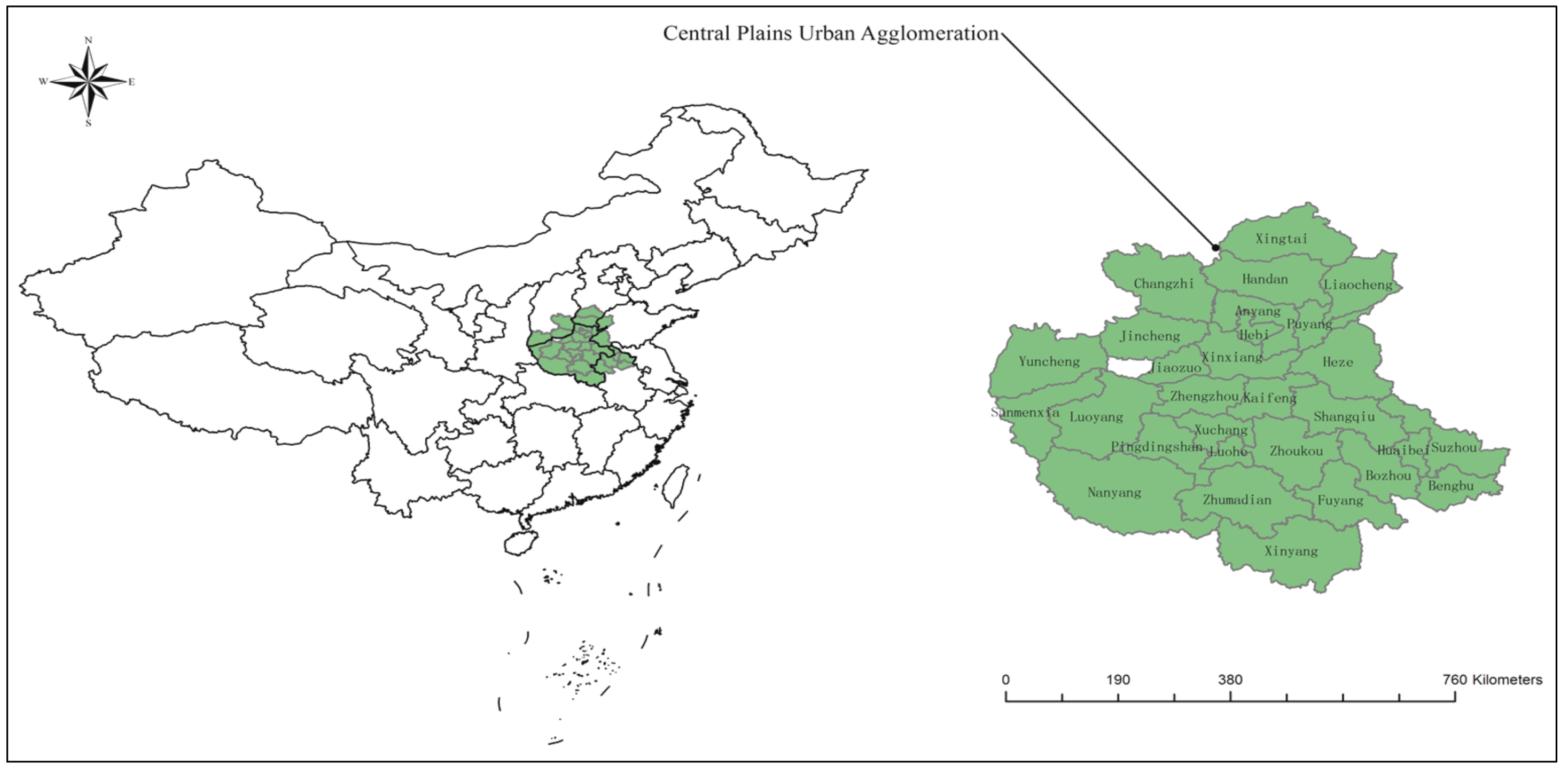
Figure 2.
The spatial distribution of industrial waste and per capita GDP in the Central Plains Urban Agglomeration (CPUA) (2004~2014). (a–d) demonstrate the distribution of wastewater discharge, industrial SO2, industrial dust, and average per capita GDP.
Figure 2.
The spatial distribution of industrial waste and per capita GDP in the Central Plains Urban Agglomeration (CPUA) (2004~2014). (a–d) demonstrate the distribution of wastewater discharge, industrial SO2, industrial dust, and average per capita GDP.
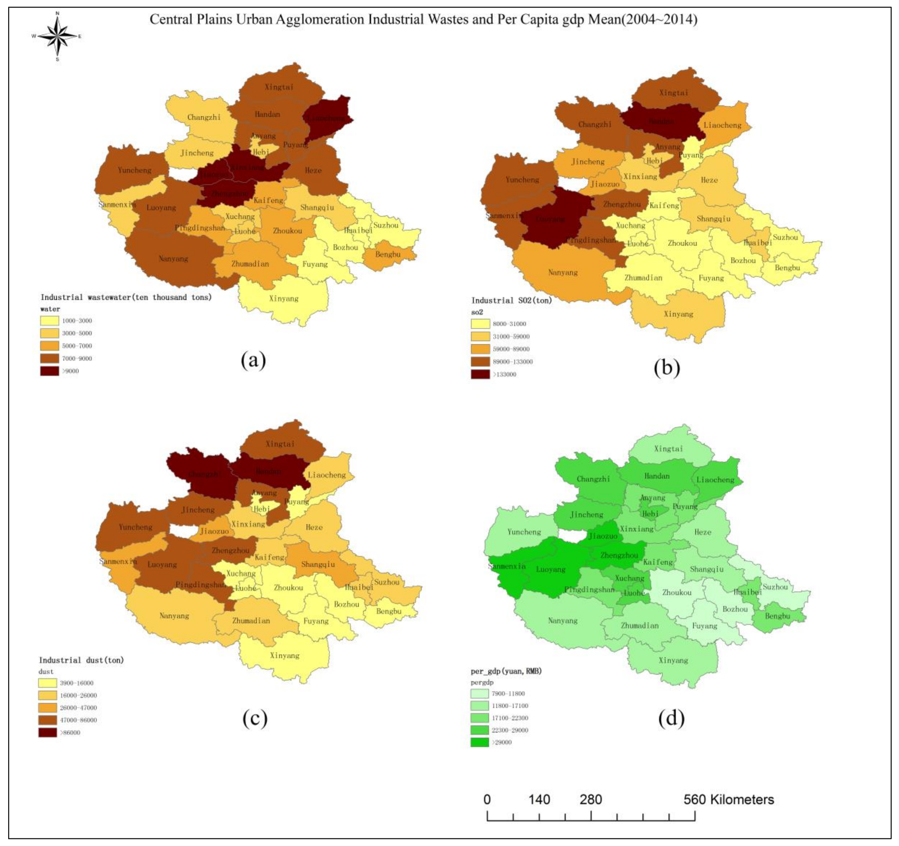
Figure 3.
The relationship between industrial pollutant discharge and the economic growth of the CPUA (a–c). Note: the horizontal and vertical coordinates are the logarithmic values of the variables.
Figure 3.
The relationship between industrial pollutant discharge and the economic growth of the CPUA (a–c). Note: the horizontal and vertical coordinates are the logarithmic values of the variables.


Table 1.
Variables’ Descriptions. GDP: gross domestic product.
| Variables Type | Variable Full Name | Abbreviation | Mean | Standard Deviation | Expected Impact Direction |
|---|---|---|---|---|---|
| Dependent variables | Quantity of industrial wastewater discharge (ten thousand tons) | Water | 7139.95 | 4475.26 | |
| Quantity of industrial SO2 discharge (ton) | SO2 | 70,455.22 | 54,423.15 | ||
| Quantity of industrial dust discharge (ton) | Dust | 39,758.97 | 41,106.06 | ||
| Independent variables | Per capita GDP (yuan) | Pgdp | 20,969.47 | 12,293.20 | + |
| Control variables | Proportion of the secondary industry in GDP (%) | Sgdp | 53.22 | 10.79 | + |
| Population (ten thousands) | People | 607.17 | 285.75 | + | |
| Foreign direct investment (ten thousand dollars) | FDI | 30,032.33 | 46,583.25 | + | |
| Technology investment (ten thousand yuan) | Tech | 16,727.57 | 21,768.38 | - | |
| Number of industrial enterprises above a designated size (number) | Factory | 881.55 | 562.58 | + |
Table 2.
Criteria for Economic Development and Environmental Pollution Assessment.
| Number | β1 | β2 | Shape |
|---|---|---|---|
| 1 | β1 = 0 | β2 = 0 | Horizontal line (unrelated relationship) |
| 2 | β1 < 0 | β2 = 0 | Monotone decreasing |
| 3 | β1 > 0 | β2 = 0 | Monotone increasing |
| 4 | β1 < 0 | β2 > 0 | “U” type |
| 5 | β1 > 0 | β2 < 0 | Inverted “U” type |
Table 3.
Results of the Variance Inflation Factor (VIF) Test.
| Variable | VIF | 1/VIF |
|---|---|---|
| Pgdp | 9.140 | 0.109 |
| Sgdp | 2.920 | 0.342 |
| People | 5.040 | 0.198 |
| FDI | 4.250 | 0.235 |
| Tech | 3.590 | 0.279 |
| Factory | 3.110 | 0.322 |
| Mean | 4.680 | / |
Table 4.
Results of Global Moran’s I.
| Year | Water | SO2 | Dust | |||
|---|---|---|---|---|---|---|
| Moran’s I | p-Value | Moran’s I | p-Value | Moran’s I | p-Value | |
| 2004 | 0.252 | 0.009 | 0.455 | 0.000 | 0.322 | 0.001 |
| 2005 | 0.216 | 0.025 | 0.426 | 0.000 | 0.348 | 0.000 |
| 2006 | 0.248 | 0.011 | 0.418 | 0.000 | 0.240 | 0.013 |
| 2007 | 0.262 | 0.007 | 0.436 | 0.000 | 0.417 | 0.000 |
| 2008 | 0.272 | 0.005 | 0.466 | 0.000 | 0.444 | 0.000 |
| 2009 | 0.253 | 0.008 | 0.449 | 0.000 | 0.394 | 0.000 |
| 2010 | 0.218 | 0.021 | 0.459 | 0.000 | 0.348 | 0.000 |
| 2011 | 0.285 | 0.004 | 0.400 | 0.000 | 0.381 | 0.000 |
| 2012 | 0.257 | 0.009 | 0.433 | 0.000 | 0.370 | 0.000 |
| 2013 | 0.238 | 0.014 | 0.440 | 0.000 | 0.368 | 0.000 |
| 2014 | 0.261 | 0.007 | 0.406 | 0.000 | 0.345 | 0.000 |
Table 5.
Regression Results of the Spatial Autoregressive Coefficient (SAC) Model.
| Variable | ln(Water) | ln(SO2) | ln(Dust) | |
|---|---|---|---|---|
| Explanatory variable | (lnPgdp) | 4.057 * | 5.625 *** | 6.670 *** |
| (1.93) | (4.37) | (3.27) | ||
| (lnPgdp)2 | −0.177 * | −0.275 *** | −0.346 *** | |
| (−1.65) | (−4.22) | (−3.15) | ||
| Control variable | Ln(Sgdp) | 1.410 ** | 0.949 ** | 0.954 |
| (2.41) | (2.10) | (1.27) | ||
| Ln(People) | 0.230 | 0.861 *** | 0.455 | |
| (0.34) | (2.95) | (0.54) | ||
| Ln(FDI) | 0.0338 | 0.0143 | 0.00237 | |
| (0.77) | (0.51) | (0.04) | ||
| Ln(Tech) | −0.105 | −0.100 * | −0.00670 | |
| (−1.46) | (−1.89) | (−0.05) | ||
| Ln(Factory) | −0.322 ** | −0.0215 | 0.0420 | |
| (−2.29) | (−0.16) | (0.17) | ||
| Spatial autoregressive coefficient | Ρ(rho) | −0.371 | −0.435 | −0.591 *** |
| (−1.32) | (−1.19) | (−3.68) | ||
| Λ(lambda) | 0.337 | 0.431 | 0.742 *** | |
| (1.34) | (1.55) | (7.28) | ||
| Variance | sigma2_e | 0.0848 *** | 0.0459 *** | 0.127 *** |
| (6.89) | (4.75) | (6.00) | ||
| Direct effect | lnPgdp | 4.206* | 6.108 *** | 7.202 *** |
| (1.90) | (3.64) | (3.18) | ||
| (lnPgdp)2 | −0.182 | −0.299 *** | −0.374 *** | |
| (−1.63) | (−3.46) | (−2.99) | ||
| Indirect effects | lnPgdp | −1.225 | −1.933 | −3.038 ** |
| (−1.04) | (−0.94) | (−2.31) | ||
| (lnPgdp)2 | 0.0518 | 0.0958 | 0.159 ** | |
| (0.96) | (0.94) | (2.16) | ||
| Total effects | lnPgdp | 2.981 * | 4.174 ** | 4.164 *** |
| (1.86) | (2.38) | (3.21) | ||
| (lnPgdp)2 | −0.131 | −0.204 ** | −0.215 *** | |
| (−1.56) | (−2.40) | (−3.18) | ||
| Curve shape | Inverted “U” type | Inverted “U” type | Inverted “U” type | |
| Turning point [95% confidence interval] | 59,874 yuan [58,519,61,228] | 22,026 yuan [20,671,23,380] | 15,994 yuan [14,639,17,348] | |
| Wald test | chi2(7) = 34.32, Prob > chi2 = 0.0000 | |||
| Lratio test | chi2(7) = 34.25, Prob > chi2 = 0.0000 | |||
| Hausman test | chi2(6) = 17.30, p = 0.0271 | |||
| Number of cities | 29 | 29 | 29 | |
| Time | 2004~2014 | 2004~2014 | 2004~2014 | |
| Sample size | 319 | 319 | 319 | |
Note: t statistics in parentheses * p < 0.1, ** p < 0.05, *** p < 0.01; [95% confidence interval] is the turning point with 95% confidence interval. Lratio: likelihood ratio.
© 2018 by the authors. Licensee MDPI, Basel, Switzerland. This article is an open access article distributed under the terms and conditions of the Creative Commons Attribution (CC BY) license (http://creativecommons.org/licenses/by/4.0/).
Share and Cite
MDPI and ACS Style
Xiong, L.; De Jong, M.; Wang, F.; Cheng, B.; Yu, C. Spatial Spillover Effects of Environmental Pollution in China’s Central Plains Urban Agglomeration. Sustainability 2018, 10, 994. https://doi.org/10.3390/su10040994
AMA Style
Xiong L, De Jong M, Wang F, Cheng B, Yu C. Spatial Spillover Effects of Environmental Pollution in China’s Central Plains Urban Agglomeration. Sustainability. 2018; 10(4):994. https://doi.org/10.3390/su10040994
Chicago/Turabian StyleXiong, Lichun, Martin De Jong, Fengting Wang, Baodong Cheng, and Chang Yu. 2018. "Spatial Spillover Effects of Environmental Pollution in China’s Central Plains Urban Agglomeration" Sustainability 10, no. 4: 994. https://doi.org/10.3390/su10040994
Note that from the first issue of 2016, this journal uses article numbers instead of page numbers. See further details here.