Article

Bayesian Approach for Estimating the Probability of Cartel Penalization under the Leniency Program

1
Department of Industrial and Management Engineering, Hanyang University, Seoul 04763, Korea
2
Department of Industrial and Management Engineering, Hanyang University ERICA, Ansan 15588, Korea
*
Author to whom correspondence should be addressed.
Sustainability 2018, 10(6), 1938; https://doi.org/10.3390/su10061938
Submission received: 30 April 2018 / Revised: 8 June 2018 / Accepted: 8 June 2018 / Published: 10 June 2018
(This article belongs to the Special Issue Risk Measures with Applications in Finance and Economics)

Abstract

:
Cartels cause tremendous damage to the market economy and disadvantage consumers by creating higher prices and lower-quality goods; moreover, they are difficult to detect. We need to prevent them through scientific analysis, which includes the determination of an indicator to explain antitrust enforcement. In particular, the probability of cartel penalization is a useful indicator for evaluating competition enforcement. This study estimates the probability of cartel penalization using a Bayesian approach. In the empirical study, the probability of cartel penalization is estimated by a Bayesian approach from the cartel data of the Department of Justice in the United States between 1970 and 2009. The probability of cartel penalization is seen as sensitive to changes in competition law, and the results have implications for market efficiency and the antitrust authority’s efforts against cartel formation and demise. The result of policy simulation shows the effectiveness of the leniency program. Antitrust enforcement is evaluated from the estimation results, and can therefore be improved.

1. Introduction

Cartels cause tremendous damage to perfect competition markets and consumers by effectually applying upward pressure on prices and downward pressure on quality; moreover, cartels are difficult to detect because of their tacit nature. In this way, cartels mitigate against perfect competition under which consumers are offered the best goods and services at the lowest possible prices. Antitrust authorities have continuously sought to maintain a free-market system against cartels, but with only partial and limited success.
In previous research, the probability of cartel detection was a key indicator for measuring the effectiveness of antitrust policies. Detection is the state in which unobserved cartels are caught by the antitrust authority. After introducing a leniency program as a new antitrust policy, both the number of cartel investigations and the probability of cartel detection increase. The higher the probability of cartel detection, the greater the expected penalties, and therefore, the likelihood of cartel formation will decrease. On this principle, it is possible to measure the deterrence effect according to the change in antitrust policy. This study uses the probability of cartel penalization as a key indicator.
The Markov transition process and the birth and death process model were widely used. Bryant and Eckard [1] constructed the birth and death process model to empirically analyze cartel data provided by the United States (US) Department of Justice, and estimated the probability of cartel detection in the US in 1961–1988 as between 13–17%. Using the same method, Combe et al. [2] estimated European Commission (EC) cartel detection probabilities of 12.9–13.2% for 1969–2007. When the birth and death model has two states of competition and collusion, the lifetimes and inter-arrival times between the births of cartels were independent and had exponential distributions with means of λ 1 and θ 1 . The number of cartels at a particular time tfollows a Poisson distribution with a mean of θ T = ( θ / λ ) { 1 e λ T } 2 . Both Bryant and Eckard [1] and Combe et al. [2] assumed that every cartel would eventually be caught and prosecuted. However, this assumption is not realistic, because some cases are not penalized, despite having been detected.
Further, Bryant and Eckard [1] and Combe et al. [2] do not take account of the unobservable cartel population. J. E. Harrington and Chang [3] sought to estimate the unobservable population by developing the birth and death model from that noted above. They concluded that cartel duration could be a good indicator of whether new competition law had a significant cartel-dissolution effect. Using Harrington and Chang [3]’s model, Zhou [4] analyzed the EC cartel data for 1985–2012, and concluded that the EU’s new leniency program in 2002 had the effect of deterring cartels.
In the research of Bryant and Eckard [1], Combe et al. [2], Harrington and Chang [3], and Zhou [4], the probability of cartel detection—as derived from cartel duration—entailed the determination of the time-average probability from continuous variables. On the other hand, there is research indicating that the probability of cartel detection represents the ensemble-average probability obtained from discrete variables such as caseloads. The time-average probability is the average of a stochastic process that is obtained by selecting a sample path randomly, and taking the average of a period in a particular state on that sample path over the observation period. The ensemble-average probability is that mean of a quantity at time t that is estimated by the average of the ensemble of possible states of total sample paths in stochastic process theory [5,6].
Miller [7] formulated a cartel behavior model using the Markov process, and used the number of cartel cases as discrete variables. The model assumed that the cartel transition process is in a non-absorbing and first-order Markov chain in contrast with previous Markov models, and showed the change of the number of cartel detections before and after a leniency program. He concluded that the introduction of this leniency program in 1993 increased the detection and deterrence capabilities of competition enforcement. The previous research above [1,2,3,4,7] used Markov process models; this research had two notable points.
First, the duration of cartels and inter-arrival times between cartels follow exponential distributions. Verifying this assumption requires a hypothesis testing of the null hypothesis that “the distribution is exponential”. The cumulative distribution function F ^ ( x ) of durations and inter-arrival times is given by:
F ^ ( x ) = n u m b e r   o f   o b s e r v a t i o n s x t o t a l   n u m b e r   o f   o b s e r v a t i o n s
Under the exponential distribution, l o g ( 1 F ^ ( x ) ) should be approximately linear in x. The result of these previous works indicates that the cartels’ duration and inter-arrival times between cartels follow the exponential distribution; therefore, models can be applied to the Markov process [7].
Second, this research assumed that the cartel process was stationary for adopting the Markov process, and that the values could be analyzed when the cartel process attained a steady state; this is also unrealistic. In the research of Bryant and Eckard [1] and Combe et al. [2], the probability is the resultant value when it reaches a steady state. This kind of probability is called a time-independent probability. Otherwise, the form of estimators needs to be a time-dependent rather than time-independent, because the purpose of estimating the probability of cartel detection is evaluating the effects of various competition policies [8]. Thus, Hinloopen [8]’s research was an theoretical literature review for analyzing a subgame of collusion.
A new mathematical methodology has emerged recently in the form of a non-Markov process. Ormosi [9] estimated the annual probability of cartel detection by employing capture–recapture methods based on EC information in the period between 1981–2001. The methods of Ormosi [9], which are frequently used in ecology, reflect that transition parameters are not steady state, and that detection and survival rates are time-independent. However, there are two unreasonable assumptions. First, capture–recapture methods assume that temporary migrations between the two states (compete–collude) do not exist; thus, they are regarded as robust design methods. The antitrust policy tends to vary broadly according to governmental power or social issues. Second, Ormosi [9] deduced a result from moving average methods, specifically in the moving average of three or five years. If the probability is used on the basis of a single year, the accuracy of the probability may decrease due to data insufficiency. The industry reacts immediately to changes in competition law; therefore, the probability needs to be estimated for the smallest unit of time.
This paper seeks to estimate the probability of cartel penalization using a Bayesian approach and evaluate the impact of the leniency program as an antitrust policy. This study uses the conjugate family of the beta-binomial in that the cartel occurs in binomial events. The posterior mean of the beta distribution is the probability of cartel penalization in a year. This shows the trend of the probability of cartel penalization, and can then improve the antitrust policy using the measured impact of the leniency program. In this light, the present research makes three contributions.
First, this paper estimates the probability of cartel penalization for analyzing cartels in contrast to the probability of cartel detection as treated in previous research. The probability of cartel detection means the probability that unobserved cartels will be investigated, prosecuted, and penalized. However, the probability of cartel penalization means the penalized likelihood of investigated cartels through sufficient investigation. This is used as an indicator with which to evaluate the impact of the leniency program and the capability of antitrust authorities.
Second, the methodology of this paper makes up for the weak points of previous probability estimation methods. Previous methods have many unrealistic assumptions such as the analyzed cases being eventually caught/detected cases, the time-average probability, etc. We can improve on these assumptions by estimating the time-dependent ensemble-average probability based on the discrete data of caseloads, which is more practical than the time-average probability for the sensitive estimation of probability.
Third, this study shows that the Bayesian approach could play a practical role in modeling and analyzing the cartel situation. Although the Markov process model, which was commonly used in previous research, is an essential consideration “in steady-state probability”, it is difficult to assume “in steady-state probability”, because cartel cases continuously vary over time. The probability of cartel penalization estimated using the Bayesian approach does not need to consider “steady-state probability”. The Bayesian approach for estimating probability can contain significant uncertainty, but has good predictive performance in itself [10]. The bias between the estimation probability and the actual value could be solved from the update procedure of the Bayesian approach. Therefore, we present reliable results using the non-informative prior and conjugate prior distribution when prior information is insufficient.
The paper is organized as follows: Section 2 defines the penalization probability and Bayesian probabilistic model; Section 3 presents an empirical study based on US cartel data; and Section 4 draws conclusions.

2. Bayesian Probabilistic Model

When faced with suspected cartel cases, a competition authority carries out an initial investigation to determine whether there are sufficient grounds to prosecute. Prosecuted cartels are penalized in the form of fines through a trial. Eventually, the three states of cartel cases are investigation, prosecution, and penalization [11]. The estimated probability of this study is based on investigation and penalization states. The probability of cartel penalization (ρt) is described as the proportion of the numbers of penalized cases to investigated cases for year t ( t = 1 , 2 , ).
The estimation of the penalization probability using the Bayesian approach involves two assumptions. First, the unit of case is an industry. Accordingly, the research of Bryant and Eckard [1] and Miller [7] is based on the analysis unit of the industry. Bos and Harrington [12] argued that firm-based analysis is more realistic; nonetheless, this study was analyzed based on the analysis unit of industry for easy analysis. In practice, cartels can participate in all firms of an industry. Second, a cartel only arises as one event during a year. Every cartel is transferred to the competition as a result of punishment by the authorities. This is called the “Grim trigger strategy” [13,14]. Thereafter, if some player deviates from the cartel, the game cannot be colluded indefinitely.
This study constructed a Bayesian probabilistic model to estimate the probability of cartel penalization. The probability of cartel penalization is the posterior mean calculated from the posterior distribution. Inferring a posterior distribution requires determining the proper prior distribution. A Bayesian probabilistic model is comprised of a prior distribution to induce a posterior distribution, hyperparameters, and a likelihood function. A Bayesian sequential analysis of the dynamic Bayesian model can be used to reflect the latest trends of time-series data [15,16].
Two things should be considered to induce a posterior distribution from a prior distribution: the likelihood function and the parameters in the prior distribution, which are known as hyperparameters [17]. The natural conjugate priors are generally recommended in the Bayesian approach, because its functional form is similar to the likelihood distribution [18,19]. Therefore, we have to obtain the appropriate likelihood function to adopt the notion of natural conjugacy. Consider the following notations for the Bayesian probabilistic model.
  • ρt: The probability of cartel penalization cases in year t
  • nt: The number of cartel investigation cases by the competition authority in year t
  • kt: The number of cartel penalization cases by the competition authority in year t
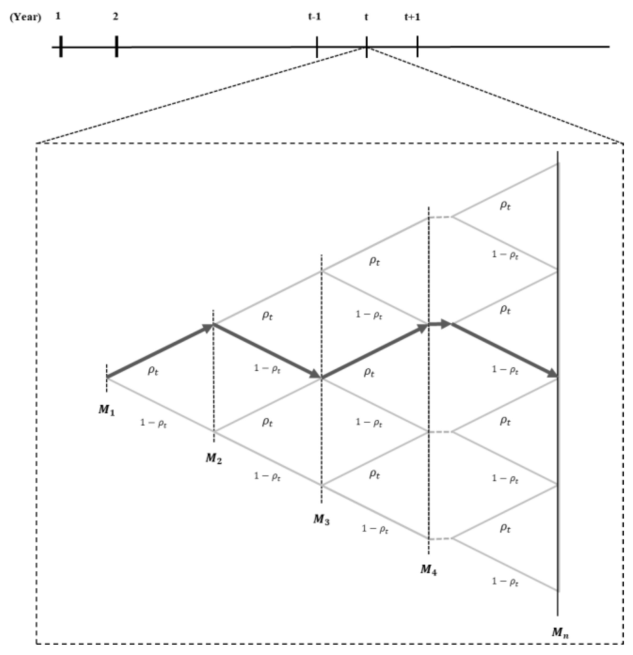
When the investigated industry participating in a cartel is n, Figure 1 shows a binomial tree to demonstrate the process of cartel formation and demise in year t.
In Figure 1, M 1 ,   M 2 , , M n is the industry of investigated cartels in year t. Arrows in the path show whether the investigated cartels were finally penalized. When a route contains an arrow pointing to the right, this cartel will be finally penalized; otherwise, it is not penalized. For example, the industry M 2 is in the left direction; this means that industry M 2 will be not finally penalized as the probability ρt. This study wants to infer the probability of industry n + 1 penalization in path G; this probability is estimating the likelihood function based on the data from industry 1 to n, and the prior distribution while inferring a posterior distribution from the Bayesian approach [13]. The expectation of a posterior distribution indicates the probability of cartel penalization.

2.1. Likelihood Function and Prior Distribution

The variable nt is the number of cartel cases investigated in year t, and each case follows the Bernoulli process with an independent and identical distribution. Therefore, the Bernoulli random variable X i with one case shown is given by:
X i = { 1 if penalizing with probability ρ t 0 if non - penalizing with probability    1 ρ t ,
where i is the number of cartel firm ( i = 1 , , n t ) and 0 < ρ t < 1 . The probability mass function of the random variable, which is known as the Bernoulli probability, is given by:
f ( x i | ρ t ) = ρ t x i ( 1 ρ t ) 1 x i .
Once the number of cases nt is investigated, and kt is penalized in year t, the joint probability mass function of cartel cases is given by:
L ( ρ t | x 1 , , x n t ) = f ( x 1 , , x n t | ρ t ) = i = 1 n t f ( x i | ρ t ) = i = 1 n t ρ t x i ( 1 ρ t ) 1 x i = ρ t x i ( 1 ρ t ) n t x i = ρ t k t ( 1 ρ t ) n t k t .
The probability of cartel penalization has a value between 0 and 1. In Equation (2), f ( ρ t ) is a binomial form as the prior distribution, because there are only two final states of a cartel: whether it has been penalized or not. Thus, we use the beta distribution as a prior distribution based on the natural conjugacy [17,20]. The prior distribution f ( ρ t ) is the beta distribution with hyperparameters α and β; thus, the probability density function is given by:
f ( ρ t ) = Γ ( α + β ) Γ ( α ) Γ ( β ) ρ t α 1 ( 1 ρ t ) β 1 ,
where α > 0 and β > 0 are the hyperparameters. The function Γ ( ) is a gamma function, which is defined as:
Γ ( α ) = 0 e x x α 1 d x .
Note that when α is a positive integer, Γ ( α ) = ( α 1 ) ! .

2.2. Bayesian Estimation

In the Bayesian approach, the posterior distribution is given by:
f ( ρ t | x 1 , , x n t ) = f ( x 1 , , x n t , ρ t ) f ( x 1 , , x n t ) .
The joint probability distribution f ( x 1 , , x n t , ρ t ) in Equation (5), which reflects the multiplicative laws of probability in Equations (2) and (3), is:
f ( x 1 , , x n t , ρ t ) = f ( x 1 , , x n t | ρ t ) f ( ρ t ) = Γ ( α + β ) Γ ( α ) Γ ( β ) ρ t k t + α 1 ( 1 ρ t ) n t k t + β 1 .
The marginal probability distribution f ( x 1 , , x n t ) , which is calculated by the law of total probability, is given by:
f ( x 1 , , x n t ) = 0 1 f ( x 1 , , x n t , ρ t ) d ρ t = 0 1 Γ ( α + β ) Γ ( α ) Γ ( β ) ρ t k t + α 1 ( 1 ρ t ) n t k t + β 1 d ρ t = Γ ( α + β ) Γ ( α ) Γ ( β ) 0 1 ρ t k t + α 1 ( 1 ρ t ) n t k t + β 1 d ρ t ,
where 0 1 ρ t k t + α 1 ( 1 ρ t ) n t k t + β 1 d ρ t = Γ ( α + k t ) Γ ( n t k t + β ) Γ ( α + β + n t ) .
Suppose that the initial probability (ρt) is 0.5 meaning whether the investigated or the non- investigated case for eliminating the dependence on the prior information. The hyperparameters α and β are 1 as a non-informative prior. Therefore, the posterior distribution is a beta distribution with the parameters α + k t and β + n t k t . The posterior distribution of Equation (5) is represented by:
f ( ρ t | x 1 , , x n t ) = f ( x 1 , , x n t , ρ t ) f ( x 1 , , x n t ) = Γ ( α + β ) Γ ( α ) Γ ( β ) ρ t k t + α 1 ( 1 ρ t ) n t k t + β 1 Γ ( α + β ) Γ ( α ) Γ ( β ) Γ ( α + k t ) Γ ( n t k t + β ) Γ ( α + β + n t ) = Γ ( α + β + n t ) Γ ( α + k t ) Γ ( β + n t k t ) ρ t k t + α 1 ( 1 ρ t ) n t k t + β 1 .
The posterior mean E [ ρ t | x 1 , , x n t ]    from Equation (8) is:
E [ ρ t | x 1 , , x n t ] = 0 1 ρ t f ( ρ t | x 1 , , x n t )    d ρ t = 0 1 ρ t Γ ( α + β + n t ) Γ ( α + k t ) Γ ( β + n t k t ) ρ t k t + α 1 ( 1 ρ t ) n t k t + β 1 d ρ t = Γ ( α + β + n t ) Γ ( α + k t ) Γ ( β + n t k t ) 0 1 ρ t ( k t + α + 1 ) 1 ( 1 ρ t ) ( n t k t + β ) 1 d ρ t = Γ ( α + β + n t ) Γ ( α + k t ) Γ ( β + n t k t ) Γ ( α + k t + 1 ) Γ ( n t k t + β ) Γ ( α + β + n t + 1 ) = α + k t α + β + n t .

3. Empirical Study

3.1. Data

This study uses data from the Workload statistics published by the Antitrust Division of the Department of Justice (DOJ) for the period between 1970–2009 [21]. The information is shown in Table 1. It contains the annual statistics of penalized cases and investigated cases by the criminal enforcement and civil enforcement of district courts, with respect to the laws of Sherman §1-Restraint of Trade, Sherman §2-Monopoly, and Clayton §7-Mergers. The antitrust division prosecutes in the form of criminal enforcement cases if the cartels, which are known as “hardcore cartels,” are determined by preliminary examination to have an especially injurious impact on the industry; otherwise, it prosecutes in the form of civil enforcement cases. This study does not consider the appellate cases and the cases of contemporary criminal–civil enforcement at the same time, due to a few of applicable cases.

3.2. Time-Series Analysis

Prior to the model application, a time-series analysis was implemented to eliminate spurious relations. This study, alternatively, employed the augmented Dickey–Fuller (ADF) unit root test to confirm the stability of the time-series data (details are provided in Appendix A).
If the result shows that the time-series data is unstable, the difference stationary process is needed. The representative method for stabilizing time-series data is order difference or log order difference. However, using order difference, it is possible that the meaning of original data will be lost, leading to different conclusions in the economy [22]. Economic variables such as price, currency, and stock index cannot be used to verify the stability of time-series data, because they are commonly non-stationary data [23].

3.3. Results

The empirical study, using the model defined in Section 2, drew an annual beta distribution for the probability of cartel penalization. The results are summarized in Table 2, and Figure 2 illustrates the distribution for every year.
Figure 2 shows that the probability distributions tend to increase over time. Beta distributions converge on a specific range with Bayesian updating [17]. Indeed, the result shows the convergence of the present distribution on the specific range at around 0.22. We were able to calculate the posterior mean by Equation (9). Figure 3, accordingly, illustrates the annual expected probability of cartel penalization.
In the late 19th century, the United States was confronted with a very significant change: large-scale manufacturing interests emerged, in great numbers, and enjoyed excessive economic power. In response, the Interstate Commerce Act in 1887 began a shift towards federal rather than state regulation of big business. This was followed by the Sherman Antitrust Act in 1890, which is the basis of US competition laws. Later, the Clayton Antitrust Act in 1914 was enacted to prohibit price discrimination, corporate mergers, and interlocking directorates.
We can now show how the change of probability of cartel penalization impacted upon the antitrust laws in the analysis periods. The Antitrust Penalty and Procedure Act in 1974, which was known as the Tunney Act, required that prospective mergers and acquisitions obtain approval from the DOJ. In 1976, the Hart–Scott–Rodino Antitrust Improvements Act was passed, and in 1978, the leniency program was instituted. At this notable time, the probability of cartel penalization was increasing. At the peak of cartel penalization probability, in 1994, the DOJ reformed the leniency program. The reformed version of the program included an additional amnesty for those who cooperate with investigations. Figure 3 indicates that the probability after 1994 has been steady and stable. The reform of competition laws clearly had an impact on the industry.

3.4. Model Comparison

Chang and Harrington [24] constructed a Markov process model to consider the stochastic formation and demise of cartels. By numerical analysis, they estimated the impact of the leniency program on the steady-state rate. Figure 4, in the form of the analysis results, plots the change in the rate of penalized cartels according to the proportion of prosecuted cases.
The proportion of probable prosecution cases, as reflects the 1970–2009 Workload statistics, was about 20~40%. In this value, the rate of penalized cartels is estimated about 5~10%.
The estimated probability of cartel penalization of this study and Bryant and Eckard [1]’s results are similar in their proportion of penalization to investigation. However, the present approach is the ensemble-average probability using discrete data, whereas that of Bryant and Eckard [1] is the time-average probability using continuous data. Cartel analysis is more commensurate with discrete data than with continuous data, because the form of Workload statistics data, as announced annually by the DOJ, is discrete. With our similar definition of probability, we could draw a box plot in the overlapped analysis period 1962–1988.
Figure 5 shows that the Bayesian probabilistic model estimates 0.114 for the top 25th percentile, and 0.1737 for the top 75th percentile, which are statistically significant. These are close to Bryant and Eckard [1]’s estimates, which fell between 0.128 and 0.174.

3.5. Impact of Leniency Program

This study utilized a policy simulation to analyze the impact of competition policies [25,26]. In policy evaluation research, the impact of policy implementation is indicated as value-added. In other words, the impact is described as the difference of outcomes between implementing the policy and otherwise. The leniency program has been deemed an effective antitrust policy for detecting and deterring cartels in many countries. In general, the leniency program provides partial or total exemption for penalty to a cartel member who voluntarily reports information or agreements that prove helpful to the antitrust authorities. Under the leniency program, a firm or individual in a cartel is bound to first confess involvement for avoiding conviction or fines. The optimal policy is found by evaluating the impact of the leniency program. It is given by:
B X 1992 A X 1992 A X 1992 × 100 .
The impact of the leniency program (%) is the difference between the penalization probability under both it and non-leniency. The leniency program was originally launched in 1978 in the US, and was reformed in 1993. In Equation (10), BX1992 is the 1992 penalization probability estimated on the basis of the leniency program’s implementation in 1978, and AX1992 is the penalization probability in 1992 estimated on the basis of the leniency program’s non-implementation. The estimated probability BX1992was calculated as 0.21211 by the Bayesian probabilistic model, and AX1992 was calculated as 0.1328 by the ordinary least squares estimation method of regression. The impact of the leniency program by the policy simulation, finally, is 65.39%. This can be seen in Figure 6.
There has been much research that has analyzed the effectiveness and efficiency of the leniency program (i.e., Miller [7], Chang and Harrington [24], and Brenner [27]). The result of this study is similar to those of the research of Chang and Harrington [24] and Miller [7], which is based on US data; the implication was that the leniency program is a very effective policy. Chang and Harrington [24] argue that the occurrence of cartels decreased by about 70%, and the deterrence capability of the antitrust authority increased by about 60% after introducing the leniency program. Miller [7], through Poisson regression analysis, estimated the impact of the leniency program every half year using US data for the years 1985 to 2005. In the results, the detection capability increased by about 60%, and the deterrence capability improved by about 40%.

4. Conclusions

This study attempted to estimate the probability of cartel penalization using a Bayesian approach. Bryant and Eckard [1], Combe et al. [2], Harrington and Chang [3], and Zhou [4] estimated the probability of cartel detection in the form of the time-average probability from continuous data. However, the probability of cartel penalization of this study was estimated in the form of the ensemble-average probability from Workload statistics. Bryant and Eckard [1], Combe et al. [2], Harrington and Chang [3], Zhou [4], and Miller [7] all assumed that the duration of cartels and the inter-arrival times between cartels follow exponential distributions, and that the stochastic process for cartel cases is stationary. However, we built a Bayesian probabilistic model, as it did not need to consider a stationary process. This study made two assumptions: an industry-based analysis, and the grim trigger strategy. On the basis of the 1970–2009 Workload statistics from the US Department of Justice, the determined probability of cartel penalization reflected a sensitive response according to the change of antitrust policy. The result of the policy simulation of the impact of the leniency program was about 65%. The results are similar with the results of Chang and Harrington [24] and Miller [7], and similar to that of Bryant and Eckard [
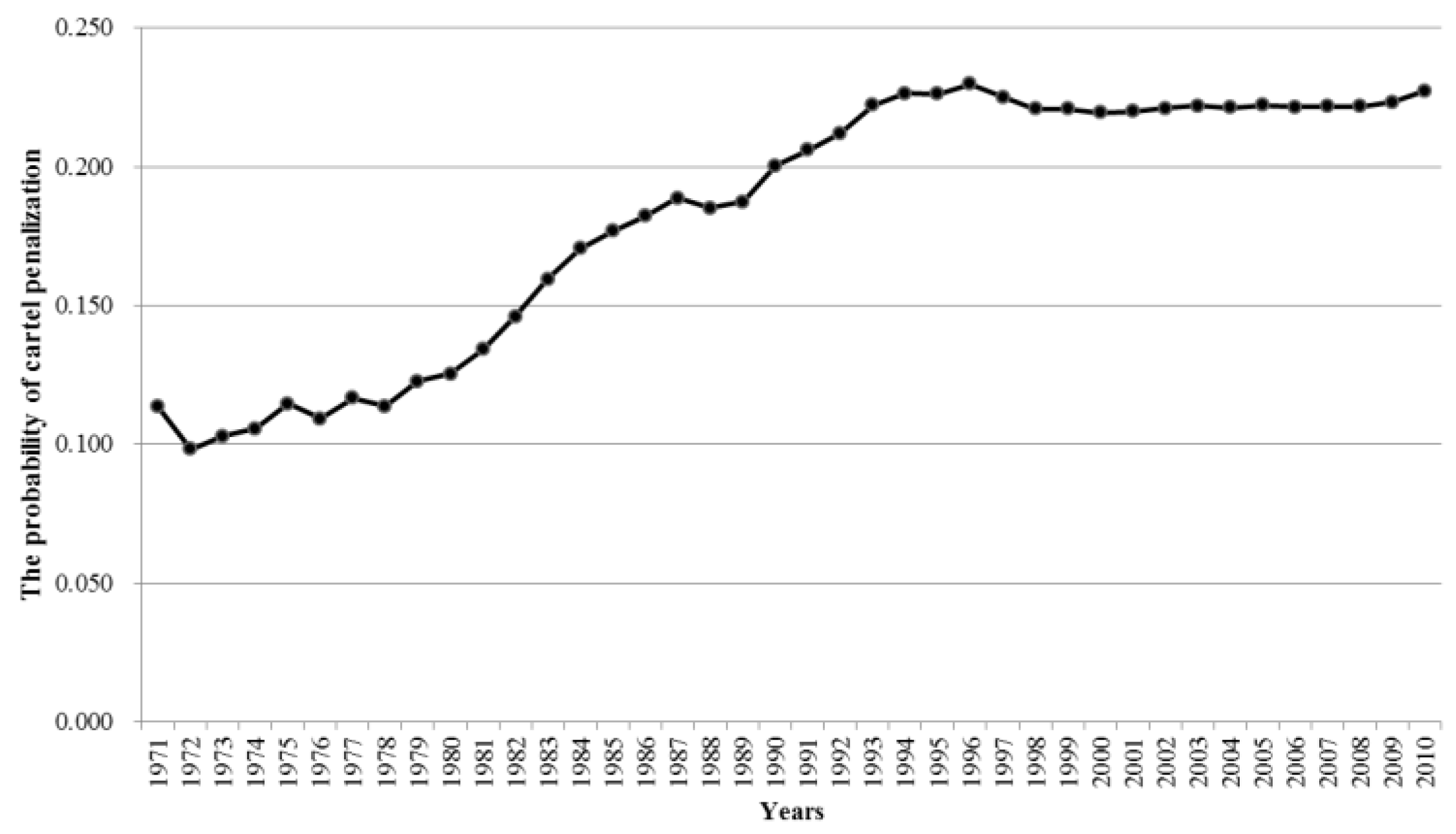
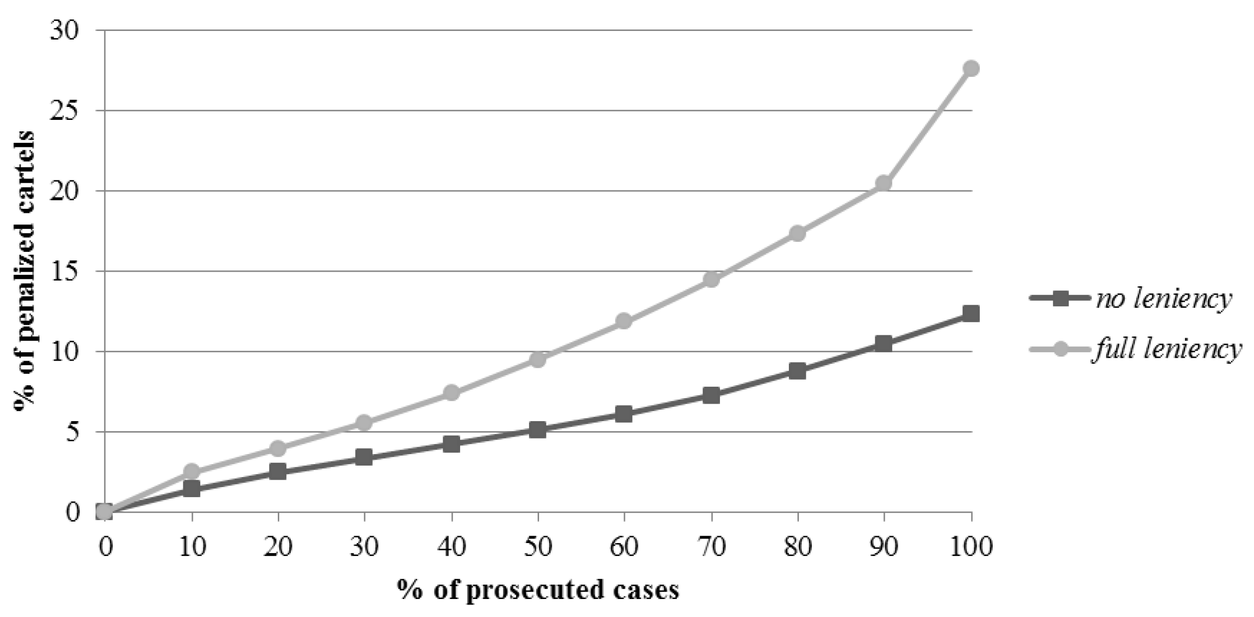
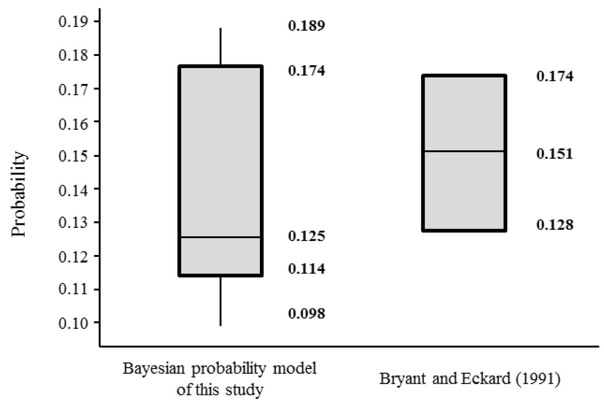
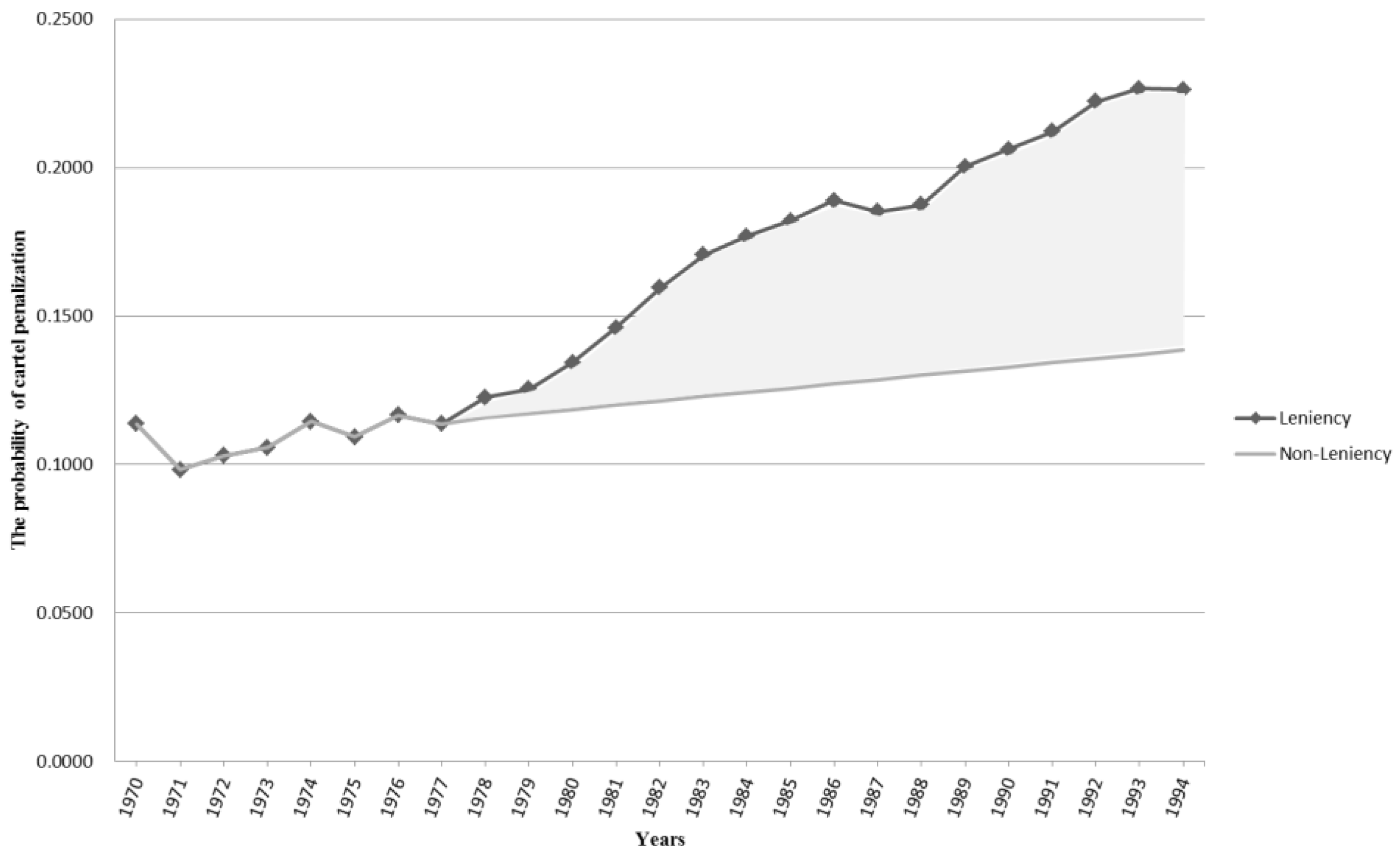
1]; indeed, the common finding among all of the studies, including the current study, was that the leniency program is a very effective policy.
This study evaluated the impact of antitrust policy and, therefrom estimated the probability of cartel penalization. From the antitrust authority standpoint, it provides an improved optimal policy, and from the corporate standpoint, it provides more effective decision-making. Certainly, the present paper has several limitations. First, further studies on realistic situations in specific countries and industries are needed. New antitrust policies recently have been introduced, such as for example, Amnesty Plus, punitive damage, class action, and consent order. These were also considered in further study.

Author Contributions

J.P., J.L. and S.A. conceived and designed the research; J.P. and J.L. conducted the research and drafted the manuscript. S.A. supervised the overall work. All authors read and approved the final manuscript.

Funding

This work was supported by the National Research Foundation of Korea(NRF) grant funded by the Korea government(MSIP) (No. NRF-2018R1A2B6003232).This work was supported by the National Research Foundation of Korea(NRF) grant funded by the Korea government(MSIP) (No. NRF-2018R1A2B6003232).

Conflicts of Interest

The authors declare no conflicts of interest.

Appendix A

An ADF unit root test of maximum time lag 10 based on the Schwarz information criterion is performed using E-Views software. The regression of the time series for the test is
y t = δ y t 1 + u t ,
where u t is the white noise error term, following the normal distribution of mean 0 and variance σ 2 .
The case of δ = 1 in Equation (A1) indicates that the model has a unit root with a random walk. Time lags usually account for one-third of the total time series [22]. Accordingly, in the ADF unit root test, the time series is 30, and so the maximum time lag is 10. In any ADF unit root test, the procedure is important [28,29]. Such procedures are the model including the constant and time trend ( y t = β 0 + β 1 t + δ y t 1 + u t ), the model including the constant ( y t = β 1 t + δ y t 1 + u t ), and the model including nothing ( y t = δ y t 1 + u t ).
There are information criteria for ADF unit root tests: the AIC (Akaike information criterion), and the above-noted SIC (Schwarz information criterion). SIC, which supplements the AIC with the Bayesian view, is mainly used in empirical analysis, and is also known as the Bayesian information criterion [30].
A I C = e 2 k / n R S S n , S I C = n k / n R S S n ,
where k is the number of regressors, n is the number of observations and RSS (residual sum of squares) is the sum of square error between the data. The null hypothesis for the ADF unit root test is “including a unit root ( δ = 1 ).” Initially, the present study used the ADF unit root test with the model including the constant and time trend based on the detection cases data. The results are provided in Table A1.
Table A1. ADF unit root test with the model including constant and time trend based on the detection cases data.
t-StatisticProb.
Augmented Dickey-Fuller test statistic−2.9816910.1501
Test critical values:1% level −4.211868
5% level −3.529758
10% level −3.196411
VariableCoefficientStd. Errort-StatisticProb.
Detection cases (−1)−0.3915320.131312−2.9816910.0051
Constant156.654960.878092.5732550.0143
@TREND (1970)−2.3072191.308371−1.7634280.0863
Table A1 shows that the p-value of the ADF test statistic, 0.1501, is greater than the significance level (0.05). This means that the null hypothesis cannot be rejected (the detection cases data has a unit root). Testing of the constant and time trend can show variable Constant and @TREND in the below of Table A2. The p-value of the constant is about 0.0143, smaller than the significance level (0.05). That is, the null hypothesis “no constant ( β 0 = 0 )” can be rejected. The p-value of the trend is 0.0863, again greater than the significance level (0.05). That is, the null hypothesis “no time trend ( β 1 = 0 )” also cannot be rejected. The time series data on the detection cases includes the unit root as well as the. Because of the lack of any time trend, we progress to the next step, which is the ADF unit root test with the model including only the constant. The results of this test are summarized in Table A2.
Table A2. ADF unit root test with the model including constant based on the detection cases data.
t-StatisticProb.
Augmented Dickey-Fuller test statistic−2.3434690.1641
Test critical values:1% level −3.610453
5% level −2.938987
10% level −2.607932
VariableCoefficientStd. Errort-StatisticProb.
Detection cases (−1)−0.2452240.104641−2.3434690.0246
Constant66.2539333.757761.9626280.0572
Table A2 shows that the p-value of the ADF test statistic is 0.1641, greater than the significance level (0.05). This result means that the data has a unit root. The p-value for constant is 0.0572, again greater than significance level (0.05). That is, the null hypothesis ( β 0 = 0 ) cannot be rejected. The time series data on the detection cases includes the unit root. Because of no constant, we progress to the final step, which is the ADF unit root test with the model including nothing. The results of the ADF root test are summarized in Table A3.
Table A3. ADF unit root test with the model including nothing based on the detection cases data.
t-StatisticProb.
Augmented Dickey-Fuller test statistic−1.3962530.1487
Test critical values:1% level −2.625606
5% level −1.949609
10% level −1.611593
VariableCoefficientStd. Errort-StatisticProb.
Detection cases (−1)−0.0526580.037714−1.3962530.1707
R-squared0.038594Mean dependent var−7.923077
Adjusted R-squared0.038594S.D. dependent var77.49139
S.E. of regression75.98132Akaike info criterion11.52416
Sum squared resid219380.1Schwarz criterion11.56681
Log likelihood−223.7211Hannan-Quinn criter.11.53946
Durbin-Watson stat2.689882
Table A3 shows that the Durbin-Watson statistic is 2.689882 where k = 1 and n = 30 . The significance level (0.05) of these variables sets up as d L = 1.352 , d U = 1.489 . The null hypothesis “serially uncorrelated” can be rejected, because DW statistics ( d ) is included between 4 d L and 4. The data on detection cases presents an eventually negative correlation. p-value of the ADF test statistic is 0.1487, greater than the significance level (0.05). This result means that the data has a unit root. In conclusion, the time series data on the detection cases includes the unit root and does not include constant and time trend. In the sequence analysis, we also use an ADF unit root test with the model including the constant and time trend based on the penalization cases data. The results are summarized in Table A4.
Table A4. ADF unit root test with the model including constant and time trend based on the penalization cases data.
t-StatisticProb.
Augmented Dickey-Fuller test statistic−2.1895360.4808
Test critical values:1% level −4.234972
5% level −3.540328
10% level −3.202445
VariableCoefficientStd. Errort-StatisticProb.
Penalization cases (−1)−0.4721170.215624−2.1895360.0365
D (Penalization cases (−1))−0.1588010.238570−0.6656370.5107
D (Penalization cases (−2))−0.2427380.210821−1.1513950.2587
D (Penalization cases (−3))0.2435270.1829941.3307960.1933
Constant38.1191618.034662.1136600.0430
@TREND (1970)−0.2339030.352704−0.6631710.5123
Table A4 shows that the p-value of the ADF test statistic, 0.4808, which is very much greater than the significance level (0.05). This means that the null hypothesis cannot be rejected (the penalization cases data has a unit root). The p-value of the constant is about 0.0043, smaller than the significance level (0.05). The p-value of the trend is 0.5123, greater than the significance level (0.05). The time series data on the penalization cases includes the unit root as well as the constant with the model including the constant and time trend. Because of the lack of any time trend, we progress to the next step, which is the ADF unit root test with the model including only the constant. The results of this test are summarized in Table A5.
Table A5. ADF unit root test with the model including constant based on the penalization cases data.
t-StatisticProb.
Augmented Dickey-Fuller test statistic−2.1319690.2339
Test critical values:1% level −3.626784
5% level −2.945842
10% level -2.611531
VariableCoefficientStd. Errort-StatisticProb.
Penalization cases (−1)−0.4501000.211119−2.1319690.0410
D (Penalization cases (−1))−0.1547860.236329−0.6549590.5173
D (Penalization cases (−2))−0.2292580.207934−1.1025520.2787
D (Penalization cases (−3))0.2606930.1795101.4522470.1565
Constant31.5806214.963902.1104540.0430
R-squared0.474430Mean dependent var0.611111
Adjusted R-squared0.406615S.D. dependent var27.22633
S.E. of regression20.97285Akaike info criterion9.052581
Sum squared resid13635.67Schwarz criterion9.272514
Log likelihood−157.9465Hannan-Quinn criter.9.129343
F-statistic6.995902Durbin-Watson2.098929
Prob (F-statistic)0.000391
Table A5 shows that the Durbin-Watson statistic is 2.098929 where k = 1 and n = 30 . The significance level (0.05) of these variables sets up as d L = 1.352 , d U = 1.489 . The null hypothesis “serially uncorrelated” cannot be rejected, because DW statistics ( d ) is included between d U and 4 d U . The data on penalization cases eventually resulted in no correlation. It shows that the p-value of the ADF test statistic is 0.2339 greater than the significance level (0.05). This result means that the data has a unit root. The p-value for constant is 0.043, greater than the significance level (0.05). That is, null hypothesis ( β 0 = 0 ) can be rejected. Therefore, we finish the steps. The time series data about penalization cases includes unit root and constant.

References

  1. Bryant, P.G.; Eckard, E.W. Price Fixing—The Probability of Getting Caught. Rev. Econ. Stat. 1991, 73, 531–536. [Google Scholar] [CrossRef]
  2. Combe, E.; Monnier, C.; Legal, R. Cartels: the Probability of Getting Caught in the European Union. Bruges European Economic Research (BEER) Papers 12/March 2008. Available online: http://aei.pitt.edu/58577/ (accessed on 8 June 2018).
  3. Harrington, J.E.; Chang, M.H. Modeling the Birth and Death of Cartels with an Application to Evaluating Competition Policy. J. Eur. Econ. Assoc. 2009, 7, 1400–1435. [Google Scholar] [CrossRef] [Green Version]
  4. Zhou, J. Evaluating Leniency with Missing Information on Undetected Cartels: Exploring Time-Varying Policy Impacts on Cartel Duration; TILEC Discussion Paper; Tilburg University—Tilburg Law and Economics Center (TILEC): Tilburg, The Netherlands, 2011. [Google Scholar]
  5. Gallager, R.G. Stochastic Processes: Theory for Applications; Cambridge University Press: Cambridge, UK, 2013. [Google Scholar]
  6. Li, X.R. Probability, Random Signals, and Statistics; CRC Press: Boca Raton, FL, USA, 1999. [Google Scholar]
  7. Miller, N.H. Strategic Leniency and Cartel Enforcement. Am. Econ. Rev. 2009, 99, 750–768. [Google Scholar] [CrossRef]
  8. Hinloopen, J. Internal cartel stability with time-dependent detection probabilities. Int. J. Ind. Organ. 2006, 24, 1213–1229. [Google Scholar] [CrossRef]
  9. Ormosi, P.L. A Tip of the Iceberg? The Probability of Catching Cartels. J. Appl. Econ. 2014, 29, 549–566. [Google Scholar] [CrossRef]
  10. Armstrong, J.S. Judgmental bootstrapping: Inferring experts’ rules for forecasting. In Principles of Forecasting; Springer: Berlin, Germany, 2001; pp. 171–192. [Google Scholar]
  11. Harrington, J.E. Behavioral screening and the detection of cartels. In European Competition Law Annual, 2006; Hart Publishing: Oxford, UK, 2006; pp. 51–69. [Google Scholar]
  12. Bos, I.; Harrington, J.E. Endogenous cartel formation with heterogeneous firms. Rand J. Econ. 2010, 41, 92–117. [Google Scholar] [CrossRef] [Green Version]
  13. Friedman, J.W. A non-cooperative equilibrium for supergames. Rev. Econ. Stud. 1971, 38, 1–12. [Google Scholar] [CrossRef]
  14. Harrington, J.E. Optimal corporate leniency programs. J. Ind. Econ. 2008, 56, 215–246. [Google Scholar] [CrossRef]
  15. Berger, J.O. Statistical Decision Theory and Bayesian Analysis; Springer: Berlin, Germany, 1985. [Google Scholar]
  16. Da-Silva, C.Q.; Migon, H.S.; Correia, L.T. Dynamic Bayesian beta models. Comput. Stat. Data Anal. 2011, 55, 2074–2089. [Google Scholar] [CrossRef]
  17. Gelman, A.; Carlin, J.B.; Stern, H.S.; Dunson, D.B.; Vehtari, A.; Rubin, D.B. Bayesian Data Analysis; CRC Press: Boca Raton, FL, USA, 2013. [Google Scholar]
  18. Ahn, S.E.; Park, C.S.; Kim, H.M. Hazard rate estimation of a mixture model with censored lifetimes. Stoch. Environ. Res. Risk Assess. 2006, 21, 711–716. [Google Scholar] [CrossRef]
  19. Koop, G.; Poirier, D.J. Bayesian-Analysis of Logit-Models Using Natural Conjugate Priors. J. Econ. 1993, 56, 323–340. [Google Scholar] [CrossRef]
  20. Guérin, F.; Dumon, B.; Usureau, E. Reliability estimation by Bayesian method: Definition of prior distribution using dependability study. Reliab. Eng. Syst. Saf. 2003, 82, 299–306. [Google Scholar] [CrossRef]
  21. Antitrust Division. 10-Year Workload Statistics; Department of Justice: Washington, DC, USA, 1970–2009.
  22. Gujarati, D. Basic Econometrics; MeGraw-Hill: New York, NY, USA, 2008. [Google Scholar]
  23. Nelson, C.R.; Plosser, C.R. Trends and random walks in macroeconmic time series: Some evidence and implications. J. Monet. Econ. 1982, 10, 139–162. [Google Scholar] [CrossRef]
  24. Chang, M.-H.; Harrington, J.E. The Impact of a Corporate Leniency Program on Antitrust Enforcement and Cartelization; Department of Economics, The Johns Hopkins University: Baltimore, MD, USA, 2008. [Google Scholar]
  25. Pindyck, R.S.; Rubinfeld, D.L. Econometric Models and Economic Forecasts; McGraw-Hill: New York, NY, USA, 1981. [Google Scholar]
  26. Sims, C.A. Policy Analysis with Econometric-Models. Brook. Pap. Econ. Act. 1982, 1982, 107–164. [Google Scholar] [CrossRef]
  27. Brenner, S. An empirical study of the European corporate leniency program. Int. J. Ind. Organ. 2009, 27, 639–645. [Google Scholar] [CrossRef] [Green Version]
  28. Dickey, D.A.; Rossana, R.J. PRACTITIONERS’ CORNER Cointegrated Time Series: A Guide to Estimation and Hypothesis Testing. Oxf. Bull. Econ. Stat. 2009, 56, 325–353. [Google Scholar] [CrossRef]
  29. Dolado, J.J.; Jenkinson, T.; Sosvilla-Rivero, S. Cointegration and Unit Roots. J. Econ. Surv. 1990, 4, 249–273. [Google Scholar] [CrossRef] [Green Version]
  30. Koehler, A.B.; Murphree, E.S. A Comparison of the Akaike and Schwarz Criteria for Selecting Model Order. Appl. Stat. J. R. Stat. Soc. Ser. C 1988, 37, 187–195. [Google Scholar] [CrossRef]
Figure 1. Estimating the probability of cartel penalization through a binomial tree.
Sustainability 10 01938 g001
Figure 2. Annual beta distributions of the probability of cartel penalization.
Sustainability 10 01938 g002
Figure 3. The annual probability of cartel penalization.
Sustainability 10 01938 g003
Figure 4. Effects of the proportions of penalized cartels according to the probability of prosecuted cases.
Sustainability 10 01938 g004
Figure 5. Box plots of the Bayesian probabilistic model and Bryant and Eckard’s (1991) model.
Sustainability 10 01938 g005
Figure 6. The increment of the probability of cartel penalization in US.
Sustainability 10 01938 g006
Table 1. Statistic of cartel data by the Department of Justice (DOJ) between 1970 and 2009.
Years1970–19791980–19891990–19992000–2009
Number of investigation cases4155250531451881
Total penalization cases544859780535
(Civil cases)351210161129
(Criminal cases)193649619406
Total fines ($thousand)47,712187,5481,612,9934,222,407
Table 2. The probability of cartel penalization through Bayesian sequential analysis.
Years (t)Investigation Cases (nt)Penalization Cases (kt)Prior αPrior βPosterior αPosterior βThe Expected Probability of Cartel Penalization ( ρ t )
1970 (1)473531154421
1971 (2)59351544211059630.11368
1972 (3)4655310596315813750.09831
1973 (4)53861158137521918520.10307
1974 (5)33857219185227621330.10575
1975 (6)38129276213330524850.11457
1976 (7)37464305248536927950.10932
1977 (8)48446369279541532330.11662
1978 (9)29068415323348334550.11376
1979 (10)40762483345554538000.12265
1980 (11)37789545380063440880.12543
1981 (12)25593634408872742500.13427
1982 (13)262109727425083644030.14607
1983 (14)24599836440393545490.15957
1984 (15)257809354549101547260.17050
1985 (16)2547710154726109249030.17680
1986 (17)3079810924903119051120.18215
1987 (18)2702711905112121753550.18883
1988 (19)2165512175355127255160.18518
1989 (20)22013212725516140456040.18739
1990 (21)1787714045604148157050.20034
1991 (22)1788114815705156258020.20610
1992 (23)17611315625802167558650.21211
1993 (24)2248416755865175960050.22215
1994 (25)2695817596005181762160.22656
1995 (26)2498618176216190363790.22619
1996 (27)4365919036379196267560.22978
1997 (28)4546419626756202671460.22505
1998 (29)4088920267146211574650.22089
1999 (30)3736921157465218477690.22077
2000 (31)2616421847769224879660.21943
2001 (32)2256122487966230981300.22009
2002 (33)1925023098130235982720.22119
2003 (34)2184323598272240284470.22190
2004 (35)1714624028447244885720.22140
2005 (36)2174224488572249087470.22214
2006 (37)2044824908747253889030.22159
2007 (38)1864025388903257890490.22183
2008 (39)1725825789049263691630.22173
2009 (40)1648326369163271992440.22341
2010 (41) 0.22728
Source: Workload Statistics, Department of Justice in the United States (US).

