The Principal–Agent Leasing Model of “Company + n Farmers” under Two Division Modes


School of Business Administration, South China University of Technology, Guangzhou 510640, China
*
Authors to whom correspondence should be addressed.
Sustainability 2018, 10(6), 2015; https://doi.org/10.3390/su10062015
Submission received: 30 April 2018
/
Revised: 3 June 2018
/
Accepted: 5 June 2018
/
Published: 14 June 2018
(This article belongs to the Special Issue Toward Sustainability: Supply Chain Collaboration and Governance)
Abstract
:The principal–agent leasing model consisting of one risk-neutral company and n risk-averse farmers is proposed by taking into consideration the characteristics of contract-farming and the fulfilment issues existing in the production process of agricultural products. We also discuss the optimal incentive coefficients and rents for n farmers under the two strategies of decentralization and concentration. The analysis suggests that the two division modes have no influence on the determination of the optimal effort level and the incentive coefficient of each party, and under the n farmers, the incentive coefficient given by the company to a single farmer household is not affected by the conditions of other farmer households. In terms of rent, land rent in the decentralized mode is strictly higher than land rent under the centralized mode. In the two modes of division, the total income of the company and the farmers is equal. Taking into account the randomness of the production process of agricultural products, the company will prefer to choose the centralized mode, and the farmers will tend to choose the decentralized mode in cooperation.
1. Introduction
In recent years, the “company + farmer” model has driven the steady growth of farmers’ income, and at the same time has also promoted the rapid development of China’s agricultural sector. However, with the development of this contract model, the traditional development mode for social and economic progress has resulted in crises and challenges [1], the company and farmers have also uncovered many problems in their cooperation, such as the noncirculation of information, the disadvantaged status of farmers, default problems, and so on. In the agricultural supply chain, farmers are owners of land and labour, and companies are providers of capital and technology. All have a great influence on agricultural development and social development, and they should be given extensive attention. At this stage, the problems uncovered by the cooperation between company and farmers tend to reduce the confidence of both parties in the supply chain, and this can cause waste in the production and sales of agricultural products, which is not conducive to the sustainable development of agriculture.
Many scholars have examined the above issues, such as studying how to improve the stability of the contract farming supply chain, how to change the inconsistent relationship between the traditional company and the farmers, how to increase the fulfillment rate, and so on. Ye et al. [2] analyzed the “company + farmer” supply chain coordination contract. In order to solve the problem of low fulfilment rates in cooperation, they innovated the “acquisition subsidies + market protection price + margin” coordination contract. Eaton et al. [3] put forward that the sale of products, reasonable design of contract terms, and good training for farmers are together the magic weapons to raise the performance rate. Bijman and Hendrikse [4] believed that the unequal bargaining power between companies and farmers is the key factor for farmers to establish cooperatives. Jang et al. [5] studied smallholder farmers in the United States, and showed that joining a cooperative can enable farmers to obtain more benefits in terms of farmers’ income, agricultural output, and cooperative income. Tregurtha and Vink [6] proposed that the trust relationship between the contractual parties is more efficient than a formal legal system in ensuring contract performance. Wang et al. [7] built a stylized dual channel model with price competition and demand uncertainty to characterize the main properties of a fashion supply chain.
The above research is of major significance for improving the performance rate of China’s agricultural supply chain. Most current studies address issues between companies and farmers by proposing a contract or model, while using less frequently often use the principal–agent theory or considering the problems based on bilateral efforts. Few scholars consider the lease relationship between company and farmers. However, principal–agent theory is one of the important methods for studying the coordination of industrial chain and supply chain. In addition, the leasing relationship between company and farmers can allow farmers to convert from upstream and downstream structures to subordinate structures. This form can reduce the possibility of default by both parties. At present, most scholars mainly improve the stability of supply chain contracts by constructing partners’ principal–agent relationships and corresponding incentive mechanisms [8]. Coleman [9] believed that if the parties lack the knowledge or skills to complete the task, and then entrust the other party to assist in its completion, it can be assumed that the two parties constitute a principal–agent relationship. Maskin et al. [10] studied the balance between risk avoidance levels and incentive settings of supply chain participants using principal–agent theory. Li et al. [11] constructed a principal–agent model between individual retailers and a single supplier. They analyzed the game between the two sides of the supply chain and the mechanism of different influencing factors on the commission rate and the supplier’s profit. Shen et al. [12] examined a two-echelon supply chain with one supplier and one retailer under the return policy. Roles et al. [13] believed that different contractual arrangements have an impact on the hard work and income of agents and principals. Fixed-salary contracts are optimal when the supply chain output is affected by the agent’s efforts.
The above-mentioned literature has currently studied only the supply chain between a company and a single farmer. However, the contract farming supply chain often comprises a company and multiple farmers. The supply relationship of multilateral cooperation in the supply chain is extremely complex, and each party’s interests and decisions influence each other. Most of the existing studies are conducted in the form of auction cooperation, and few scholars consider the scientific game cooperation models [14,15]. Nagarajan M et al. [16] studied a multilateral bargaining model consisting of a single buyer and multiple suppliers, and analyzed the influence of supplier rankings on their returns in bilateral negotiations, assuming each supplier cooperated in the process of the alliance. Relationships compete with each other when they compete for the order of negotiation. Based on Stackelberg game theory and when the parties to the cooperation have private cost information, Ji et al. [17] analyzed the impact of false reporting behaviour on the profit of each member of a supply chain consisting of a retailer and two competing manufacturers. Dai et al. [18] established a multiparty supply chain cooperation model using systemic coordination theory, explaining that logistics companies and supply chain members achieve synergy and that the supply chain system tends to be orderly under multilateral cooperation.
In summary, the principal–agent theory is applicable to a certain degree in the industrial chain operation mechanism and supply chain coordination research. The use of principal–agent theory at this stage is mainly reflected in the establishment of principal–agent relations and the design of appropriate incentive mechanisms to improve the overall utility of the supply chain. Therefore, based on principal–agent theory, this paper will build a leasing model of “company + n farmers”, combine the characteristics of contract farming, and consider a risk-neutral company and n risk-averse farmers’ supply chains. It also discusses the optimal incentive coefficients and rents for n farmers under the two strategies of decentralization and concentration. Next, it analyzes the decision-making behaviour of all parties in the supply chain under the principal–agent leasing model and multilateral cooperation. Lastly, it provides a valuable references for the actual operation of the agricultural supply chain.
2. The Basic Model Construction
2.1. Problem Description
From the analysis of related documents and the relationship between the company and farmers, we find that the leasing model can be introduced into the cooperation between company and farmers, and build a leasing model based on the principal–agent theory. In this model, the farmers rent their own land to the company. The company then regularly pays fixed rents to the farmers. After acquiring the land, the company entrusts the farmers to participate in crop production. In the later period, when the production cycle of agricultural products is ended, the company distributed the income from the sale of agricultural products to the farmers at a certain proportion. Under this model, the status of the farmers is transformed from traditional upstream suppliers to corporate agents. On the one hand, the farmers’ status in supply chain cooperation is enhanced. On the other hand, a reasonable incentive mechanism can be designed to reduce the default rate in the process of cooperation between the two parties.
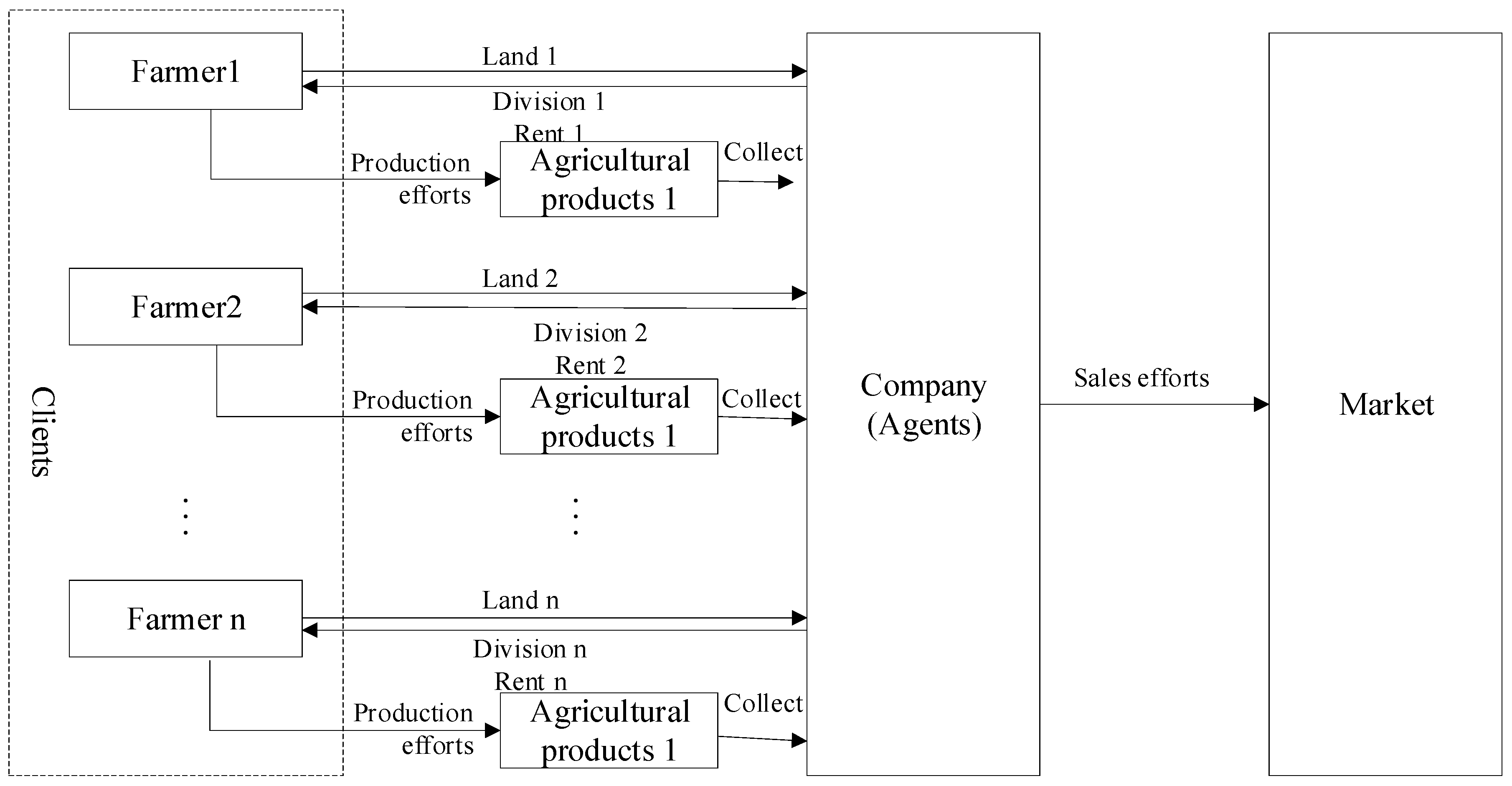
Based on the complexity of the contract farming supply chain in actual operation, this paper considers an agricultural supply chain consisting of one company and multiple farmers. In this supply chain, the company will cooperate with n () farmers who have different amounts of land, different production capacities, and different expected return levels, and determine the land rent and incentive coefficient to give each farmer. Figure 1 below shows the principal–agent leasing model for a single company and n farmers:
When considering the participation of multiple farmers in cooperation, because the output of each farmer varies, the company can divide shares in income among the farmers in two ways. The first way is, a decentralized (N-I) model: in which the company gives the farmers their share based on the proportion of the income generated by each farmer’s own agricultural products. The second way is, a centralized (N-II) model: in which the company distributes the income generated by the total agricultural products produced by n farmers to each farmer in different proportions.
Under the decentralized mode, the company signs a principal–agent lease contract with n farmers. Farmers lease their own land to the company; then, the company pays the rents of each farmer regularly, and entrusts the n farmers as employees to carry out crop production. At the end of the production cycle, the company collects the agricultural products produced by the farmers and sells them to the market. That is to say, the split income of farmers is determined by their own output and the proportion given by the company, rather than being affected by the output of other farmers.
In contrast to the decentralized sharing model, under the centralized sharing model, the company collects the output of all farmers collectively and distributes it to each farmer according to a certain percentage of the total output of all farmers. In other words, the farmers’ income depends on the total output of all n farmers and the proportion determined by the company to the farmers. In this case, the farmers’ is affected by the output of other farmers.
2.2. Model Assumption
Before building the model, we make the following assumptions.
- Consider a two-tier “company + farmer” supply chain, consisting of n farmers and a company.
- The company and farmers work together to determine the output of the supply chain. Farmers’ production efforts, such as purchasing machinery and equipment, increasing time investment, and so on, affect the output of crops. The company’s sales efforts, such as advertising and packaging products, will influence the market prices of crops.
- In the production process, agricultural products will not only be affected by the production inputs of farmers, but can also be easily damaged by external factors, leading to outstanding uncertainty in output. For example, drought, insect pests, etc., may affect the output of agricultural products. Assume that there are minimum yields for different farmers’ land, and the minimum output is the output when the farmer only sows and harvests, without expending any other effort. Land production increases with the farmers’ effort level. Therefore, suppose the farmer’s production function iswhere is the production effort level of farmer i, which is related to the human, material, and financial resources and other factors invested in planting production; represents the uncertainties caused by the natural environment or human factors; and is the effort yield coefficient of farmer i.
- The market price of agricultural products is affected by the sales effort level of the company. When the company’s sales effort invested is , the agricultural product market sales price is , and is the basic sales price.
- In terms of the microeconomic theory, the negative utility function of the company and farmers is the monotonically increasing convex function of the effort level. For convenience of calculation, it is assumed that the negative utility functions of the company and the farmers are given by the following two functions, respectively.where and are effort cost coefficients for the company and farmer i, respectively, for .
- In the principal–agent leasing model, both parties pursue the maximization of profits. Through this model, farmer i seeks to ensure a certain level of income . Assume that, in order to encourage agents to work hard in the supply chain, the principal company designs the following incentives mechanism, which is the contract with farmers.In the equation above, is the remuneration paid to farmer i by the company, and is the land rent that the company gives farmer i. Under the principal–agent leasing model with the participation of multiple farmers, is an incentive coefficient that the company gives farmer i. The higher is, the higher the return to the farmers, and ; denotes the income to farmer i from selling agricultural products, .
- Assume that the company maintains a risk-neutral attitude, and that the farmers are risk averse. The Pratt–Arrow risk premium formula shows that the absolute risk aversion coefficient is , so the risk cost of farmer i is,where is the risk aversion coefficient for farmer i, .The subscripts “c” and “f” represent the company and the farmers, respectively, throughout this paper.
2.3. “Company + n Farmers” Decentralized Mode (N-I Mode)
Under the decentralized (N-I) mode, to encourage farmers to invest more effort into the production process, the division of the company’s grants to farmers is determined by each farmer’s own output, which maximizes the benefits of each farmer and company in the model. At this point, the company, as an agent, encourages farmers to work hard and signs the following contracts with farmers.
where , and is the income from selling agricultural products produced by farmer .
This paper uses the Pratt–Arrow risk premium method to measure risk; therefore, the risk cost of the farmers is
The company and each farmer are engaged in production under the principal–agent leasing model. At this time, the income functions of each farmer and the company are
In the principal–agent leasing model, the company and the farmer both pursue the maximization of utility, and the farmer i will participate in the cooperation when their income is greater than a certain level . Therefore, we establish a principal–agent leasing model for the company and multiple farmers as follows.
(IR) is the participation constraint: only when the conditions are met will each farmer participate in the cooperation. (IC) is the incentive compatibility constraint; that is, each farmer chooses their optimal effort level according to their own benefits. Satisfying the incentive compatibility constraint means that the interests of the company and the farmer are exactly the same, and the behaviour of the farmer will meet the maximum benefit of the principal.
Let ; then, we get . Substituting into the principal–agent model, a mathematical model of a nonlinear programming problem with multiple inequality constraints is established. The Kuhn–Tucker (K–T) theorem is used to solve the extreme points of the problem. Given Lagrange multiplier , we construct the generalized Lagrangian functions, as described below.
In the equation above, , .
According to the K–T conditions, we obtain
Calculating the above equation according to the K–T conditions, we obtain the solution as follows.
Applying the above model to the supply chain formed by the company and a single farmer, calculating the results, and comparing them with the above results, it was found that the incentive coefficient, the company’s and the farmers’ effort levels, and the rent of the individual farmer were in compliance with the cooperation between the company and n farmers. We substitute the above solution result into to obtain the optimal effort level of farmer i, as follows.
According to the “Company + n Farmers” (N-I) principal–agent model established above, the optimal expressions for each farmer’s production level , company’s sales effort level , incentive coefficient , and rent are obtained.
From Equation (10), under the “company + n farmers” (N-I model), it can be seen that the incentive coefficient given by the company to different farmers depends only on the household’s own production capacity, risk aversion coefficient, and exogenous uncertainties, but nothing else. According to Equation (11), it can be seen that when working with n farmers, the company’s effort level depends on each farmer’s various factors, but has nothing to do with the minimum income required by farmers. The factors affecting rents given by the company to the farmers are the most comprehensive and are subject to the basic market price , the minimum income required by each farmer , the minimum output of the land , the risk aversion coefficient of the farmer , the uncertainty factor , the company’s effort cost factor , the farmer’s efforts , and effort cost factor .
In the case of “company + n farmers,” the impact factors of production efforts are different from those of a single farmer. The effort level of a farmer depends not only on his own land conditions, production capacity, risk aversion, etc., but also on the land conditions, production capacity, and degree of risk aversion of other farmers who are jointly involved in the cooperation. In other words, when multiple farmers participate in cooperation, a certain farmer’s decision will be affected by the production behaviour of other farmers.
2.4. “Company + n Farmers” Centralized Mode (N-II Mode)
Under the “company + n farmers” (N-II model) principal–agent leasing model, such as employees, a number of farmers sign land contracts with the company to obtain land rents, and are entrusted by the company to participate in the production and planting of agricultural products. When the final agricultural products are recovered in a unified manner, according to a certain proportion , the company distributes the income generated by selling all agricultural products to the different farmers. Here, . Assume that under the centralized sharing model, the company, as an agent, signed the following contracts with farmers:
where , and is the income from the selling agricultural products produced by farmer .
Based on the above assumptions, in the case where the n farmers are risk-averse decision-makers, all parties in the supply chain organize production in accordance with the contract, and the products are then collected together and sold by the company. The income function of farmer i is as follows.
The company’s income function is
Similarly, we establish the following proxy models for the company and multiple farmers.
Here, (IR) is the participation constraint of the principal–agent model. Only when this condition is met will each farmer be willing to participate in the cooperation. (IC) is the incentive compatibility constraint; that is, each farmer will make the best effort to maximize their own interests. When the incentive compatibility constraint is satisfied, the company’s and farmers’ interests are completely consistent, and the farmer’s behaviour will meet the principal’s maximum benefits.
In order to ensure their own benefits, farmers can determine the optimal effort level in the production process. Therefore, seeking the first derivative of for the incentive constraint (IC), we can obtain the optimal effort level of farmer i as follows.
Let ; then, we get . Substituting into the principal–agent model, we continue to use the Kuhn–Tucker theorem to solve the extreme points of the problem. Given the Lagrangian multiplier , we construct the generalized Lagrangian function as follows
where , .
According to the K–T conditions, we obtain
According to the K–T conditions, the K–T point is solved as follows.
In the same way, substituting the above solution results in , and we obtain the optimal farmer effort level as follows.
According to the “Company + n Farmers” (N-II model) principal–agent model established above, the optimal expressions for the farmers’ effort level , company’s effort level , incentive coefficient , and rent are obtained by considering the centralized mode. Below is a comparative analysis of the multiple farmers’ cooperation under the two division modes.
3. “Company + n Farmers” Models Comparative Analysis
According to the previous solution to the “company + n farmer” principal–agent leasing model in different modes, this section will discuss the differences between the optimal decision-making of the company and the farmers in the two different division modes. After a simple comparison and observation, it is found that, regardless of whether in the (N-I) or (N-II) mode, the incentive coefficient given by the company to farmer i, the level of production efforts of the farmers, and the company’s sales efforts are all equal, and they are affected by only the farmers’ own production capacity, risk aversion, and exogenous uncertainties. They have nothing to do with the impact of the farmers’ own minimum land producti on, basic market price of agricultural products, sales ability of the company, other farmers’ productivity, and minimum land production.
Proposition 1.
Under the “company + n farmers” principal–agent leasing model, as opposed to the decentralized mode, when selecting the centralized mode, parties involved in the cooperation will proceed toward the maximization of their own benefits, and the company will not change the levelof sales efforts and each farmer’s sharing ratio, i.e.,,, farmers will not change their own efforts; that is,.
Proof.
Therefore, under the two division modes, parties involved in the contract will not change their own efforts to maximize their own interests. At the same time, the company’s incentive coefficient for farmers will not change. ☐
Proposition 1 shows that whether in the decentralized or centralized mode, the company acts on self-interested terms when deciding on a principal–agent leasing contract: the proportion of shares granted to farmers and the level of self-sale efforts will not change. The investment of the farmers’ efforts in both modes depends on the proportion of shares and the company’s effort to invest, which in turn causes the farmers to not change their effort level.
Proposition 2.
Under the “company + n farmers” principal–agent leasing model, the land rents received by the farmers under the decentralized mode of agricultural products are always higher than the land rents collected by the farmers in a centralized mode. That is,is permanently established.
Proof.
When the company cooperates with multiple farmers, we perform an analysis of a company and farmers using the two different sharing modes, and analyze the amount of land rent that the farmers obtain. Due to , , , in the following analysis, these are uniformly expressed as , , . We compare the rents and as follows.
Thus . In other words, when the company adopts the decentralized mode in its cooperation with n farmers, the land rent paid in the previous period is higher than that obtained by adopting the centralized mode. ☐
Proposition 2 means that the difference in the division modes leads to a difference in land rent. The rent is part the company’s fixed expenses, and the share for farmers that is given in the later period may change with the change of output, the company that is the dominant party to the contract can choose different modes of division according to the funding situation in the previous period and the uncertainty of the production of agricultural products.
Proposition 3.
Under the “company + n farmers” principal–agent leasing model, whether the company adopts the agricultural product decentralized (N-I) mode or the centralized (N-II) mode to cooperate with a number of farmers, the highest benefit it receives is consistent, i.e., .
Proof.
We substitute the optimal level of production effort and incentive coefficient obtained in the two cases to analyze and compare the maximum profitability of the company under the two division modes, as follows.
Combined with the above derivation, under the premise of maximizing benefits, and from the perspective of the company, it is found that the proportion of shares given to farmers and their own sales efforts will not be changed, the effort level of all farmers remains unchanged, and the total income generated by agricultural products also remains unchanged. Compared with the (N-II) mode, under the (N-I) mode, the company more rents to the farmers in the earlier period, but the total share of the n farmers was lower in the later period. The total overpayment paid in the previous period is complementary to the total amount paid less in the later period. Thus, no matter whether the company chooses to share according to each farmer’s own production, or to collect all the farmer’s agricultural products together first and give them a different proportion of shares in the end, there is no difference in the company’s optimal total benefits. ☐
Proposition 4.
Under the “company + n farmers” principal–agent leasing model, despite whether the company adopts the agricultural product decentralized (N-I) mode or the centralized (N-II) mode to cooperate with multiple farmers, the maximum income obtained by farmers remains unchanged; that is, .
Proof.
Substituting the optimal production effort and incentive coefficients obtained under the (N-I) mode and (N-II) mode, the maximum income of the farmers under the two division modes can be analyzed and compared as follows.
☐
In summary, it can be seen that the farmers do not change their own efforts in order to maximize the benefits, and the company gives the farmer the same proportional shares. As a result, under the (N-II) mode, compared to the (N-I) mode, the income of agricultural products obtained by the farmers in the later period is higher. At this time, due to the lower land rents received by farmers in the earlier period, the sharing benefits increased in the later period are complementary to the rents missing in the previous period. As to whether the farmers choose to share according to their own production, or collect all the farmers’ agricultural products and obtain their shares in the end, there is no difference in the ratio of the proportion of farmers in the optimal total income.
Proposition 5.
Under the (N-I) and (N-II) “company + n farmers” principal–agent leasing models, the more farmers participate in the cooperation, the higher the efforts invested by the company and the farmers; that is , the bigger n, the biggerand .
Proof.
From the above derivation, it can be seen that the expression of is as follows.
Let , where and , with the increase in the number of farmers n, x and y both increase, and . Thus, when n increases, the company’s sales efforts also increase.
Again, , and does not change with the change of n, so the effort level of each farmer is an increasing function of the company’s effort level . Thus, when the number of farmers increases, the effort level of farmers also increases. ☐
In the actual situation, the company’s agricultural products will eventually increase with the increase of n. When the total output is too large, due to sales pressure, the company will definitely invest more in advertising, product packaging, quality control, and other aspects, so that agricultural products will bring higher profits.
4. Numerical Analysis
Considering the “company + n farmers” principal–agent model, due to the large number of parameters set in this section and their complex relationship, this section will select specific parameters for more intuitive comparison and analysis. According to the previous analysis, the company’s efforts with farmers are bigger than 0, the sum of the incentive coefficients is less than 1, and the rent must be bigger than 0. Therefore, the values of the parameters must satisfy the following inequalities: , , .
Consider and ; that is, numerical analysis under the “company + 2 farmers” and “company + 3 farmers” principal–agent leasing models, assuming that the effort yield coefficients of the farmers are , , and . The effort cost coefficients are , , and , respectively. The minimum demands are , , and , respectively. The minimum productions of land are , , and , respectively. The degrees of risk aversion are , , and , respectively. The company’s effort cost coefficient is , the retail market price of agricultural products is , and the exogenous uncertainty factor of variance is .
In the following table, the farmers participating in the cooperation when n = 2 are Farmer 1 and Farmer 2, and the farmers involved in the cooperation when n = 3 are Farmer 1, Farmer 2, and Farmer 3. Certainly, the corresponding parameters are consistent with the above assumptions.
As for the “company + 2 farmers” and “company + 3 farmers” principal–agent leasing models, under the decentralized mode (N-I) and the centralized mode (N-II), Table 1 lists the company’s sales efforts, the production efforts of farmer i, as well as the rent and incentive coefficient paid by the company to each farmer.
The above table shows that, when the number of farmers is fixed with various parameter assumptions—that is, n = 2 or n = 3—under the decentralized mode (N-I) and the centralized mode (N-II), these two principal–agent leasing models with n farmers, the optimal effort input of the company and the farmers stay the same, the incentive coefficient given to each farmers is also unchanged, and the total income obtained by the company and each farmer are not affected by the choice of the mode. Thus these conclusions obtained are consistent with Propositions 1, 3, and 4. In addition, only the land rent paid by the company to farmers changes with the choice of the mode, and the land rents received by different farmers from the company in the decentralized mode (N-I) are always higher than the land rents collected by farmers under the centralized mode (N-II); thus, the numerical results of this section are in agreement with Proposition 2.
Comparing the size of the decision variables with different farmers’ households, it can be seen that, despite the mode of division, when the number of farmers participating in the cooperation increases, the share ratio obtained by the same farmer remains unchanged, and the investment in production effort that needs to be paid increases. At the same time, the income received by each farmer remains unchanged. On the other hand, the company’s sales efforts increase with the increase in the number of farmers, and the company’s total benefits from the cooperation have also increased.
From the farmer’s point of view, the benefits from the choice of the two different division modes remain the same, however compared to the centralized mode (N-II), the farmers obtain higher rental income under the decentralized mode (N-I). Because the rent is paid to the farmers in the previous period, the rent can be considered a fixed income for farmers. In order to avoid the uncertainty of the latter stage of production and affect the income share of the agricultural products obtained in the later period, the farmers will prefer the decentralized mode. On the other hand, as the number of farmers participating in the cooperation increases, the effort level that the farmers need to invest is also higher, but the income obtained by each farmer does not change. At this time, the farmers tend to prefer cooperative modes comprising a smaller number of farmers.
From the company’s point of view, the total benefits obtained by choosing different division modes remain the same. If selecting the decentralized mode (N-I), the company needs to pay a large amount of land rent to the farmers in the previous period, so when the company’s funds are insufficient in the early period, the company can negotiate with the farmers for cooperation under the centralized mode. In the case of adequate funding, the decentralized mode may also affect the company’s future income due to production uncertainty. In general, adopting the centralized mode will be more beneficial to the company in a cooperation.
In this paper, under the centralization mode of n farmers, there is a benefit link between farmers, that is, the production behaviour of other farmers will affect the income and decision-making of individual farmers. In fact, when this mode was first proposed, we expected that the effort level, incentives, rents, and returns under this model would be different from the decentralized sharing mode, and would lead to an optimal cooperation mode; however, through mode solving, propositional derivation, and numerical analysis, we have found that the two models differ only in rent. Now we can explain this with the following reasons. First of all, from Equation (10) and Equation (22), when formulating contracts in the early stages, because the company cannot determine the production behavior of the farmers in the production process, it can only determine the proportion of the households through the production capacity and uncertainty factors of the households. Therefore, in the two modes, the proportion of the company’s share to each household is the same. Secondly, according to the Equations (2) and (14), under the two-share mode, although the income received by farmers is different, in the principal–agent model, peasant households as information superiors will exert their own efforts to make investment decisions according to the cooperation conditions provided by the company. Therefore, the formula for obtaining the peasant household’s effort level under the two modes is the same. Lastly, taking into account the fact that the level of production efforts of each farmer is constant under both circumstances, and the output of the final harvested agricultural products is the same, the sales efforts invested by the later companies will not change.
5. Conclusions
Considering the specific characteristics of the bilateral efforts of the company and the farmers as well as the uncertainty of agricultural output, this paper first builds a principal–agent leasing model in which a single risk-neutral company cooperates with n risk-averse farmers. Then, by solving the nonlinear programming problem with multiple inequality constraints, the optimal production effort, the company’s optimal sales effort, and the optimal contract sharing ratio and rent for each farmer are obtained. Lastly, this paper discusses the influence of the decentralized mode and the centralized mode of these two models on each decision variable. The research results show that the optimal effort level and incentive coefficients of the company and the farmers under the two division modes are equal. Among the n farmers, the incentive coefficient provided by the company to each farmer is not affected by the conditions of other farmers. However, in terms of rent, the rent paid under the decentralized mode is higher than that under the centralized mode, while the total benefits of the company and farmers under the two division modes are constant. Taking into account the uncertainty in the production process of agricultural products, the company in the cooperation will prefer the centralized mode, but the farmers will be more inclined to adopt the decentralized mode. When the number of farmers participating in the cooperation increases, the effort level invested by the company and the farmers will also increase. As a result, the cost of the farmers’ efforts will increase, but the final benefits will remain unchanged. Therefore, at this time, the farmers will tend to choose cooperation with a small number of farmers. Therefore, in regard to a cooperation between a single company and multiple farmers, the company and farmers can make decisions based on the division mode and the number of participating farmers in order to maximize their respective self interests.
Agricultural development is the foundation of China’s national economy and affects both the national economy and the people’s livelihood. This paper designs a principal–agent leasing model to transform the upstream and downstream relationships in the traditional supply chain of company and farmers into an affiliation relationship between principal and agent, which essentially changes the disadvantaged status of the farmers. In this model, the farmers’ income is not only derived from the income generated by the production of agricultural products, but also from the rental income from land leases and the distribution of profits from their own production efforts. At the same time, the model also changes the vulnerable situation in which peasant households alone bear the yield risk. To obtain higher-quality agricultural products, the company can also regulate the farmer’s production and planting behaviour while ensuring enough land and labour. In addition, taking into account the different modes in which the multi-farmer cooperation may exist, this paper has compared and explored the two modes, and has given the company and farmers a better cooperation proposal and choice. The rational use of agricultural resources has become the basis for the sustainable development of agriculture. Only by fundamentally resolving the problem of unbalanced interests between the company and farmers can we develop and utilize agricultural resources in economical and rational ways. At the same time, the increasingly sharp contradiction between supply and demand for agricultural resources will be resolved to achieve the sustainable use and development of agricultural resources.
In conjunction with this study, the following aspects should be focused on in cooperation in agricultural supply chain: (1) Change the unequal status of farmers and companies in the supply chain and better protect the rights and interests of farmers. Under the “company + farmers” model, farmers as the upper reaches of the supply chain often bear the production risk alone, and when cooperating with large-scale and strong enterprises, the negotiation ability of farmers is relatively weak. If the innovative contract model can give farmers more rights to speak and greater initiative in the production and management process, then the autonomous production will of farmers will be fully reflected; (2) All interests are diverted to ensure the sustainable development of production. Changing the “company + farmer” model, the farmers’ income comes from only the company, while the company’s interests all come from the status quo of the market, so that the interests of all parties in the supply chain comprise multiple aspects. The company and the farmers can form a win–win benefit link; (3) When multiple farmers cooperate, they can start with the benefit linkage mechanism among farmers. When cooperating with a number of farmers, the company can try to coordinate the supply chain from the perspective of optimizing revenue sharing. Through mutual encouragement between farmers, they will work together to achieve higher benefits.
Of course, the “company + farmer” contract farming supply chain is a complex system containing a variety of uncertainties, and as this paper’s research is based only on a certain simplified model, and it does have some limitations. In the future, certain aspects could be improved: (1) This paper has assumed only a fixed value for the minimum income level of farmers in the principal–agent leasing model. However, considering the actual situation, the minimum income requirement of farmers may be related to the minimum land output, farmers’ productivity, etc. Therefore, to create a decision model closer to reality, we can further try to consider the impact of these hypothetical changes on the incentive mechanism in the future based on the existing research results; (2) This paper only considers farmers’ risk aversion preferences. If companies and farmers are risk averse, how should the incentive mechanism be designed?
Author Contributions
Conceptualization, J.Y. and Y.Z.; Methodology, J.Y.; Software, X.Z. and Q.Z.; Validation, J.Y. and X.Z.; Formal Analysis, J.Y. and X.Z.; Investigation, X.Z. and Q.Z.; Resources, J.Y. and X.Z.; Data Curation, J.Y., X.Z. and Q.Z.; Writing-Original Draft Preparation, J.Y. and X.Z.; Writing-Review & Editing, J.Y., X.Z and Q.Z.; Visualization, X.Z. and Q.Z.; Supervision, J.Y. and Y.Z.; Project Administration, J.Y. and Y.Z.; Funding Acquisition, J.Y.
Funding
This research was funded by National Natural Science Foundation of China (71301054,71520107001), Guangdong Province Philosophy and Social Sciences “13th Five-Year“ Planning Project for Building Discipline of 2017 (GD17XGL56) and the Fundamental Research Funds for the Central Universities (2017X2D14, 2015QNXM13).
Conflicts of Interest
The authors declare no conflicts of interest.
References
- Wu, J.; Zhang, X.; Lu, J. Empirical research on influencing factors of sustainable supply chain management—Evidence from Beijing, China. Sustainability 2018, 10, 1595. [Google Scholar] [CrossRef]
- Ye, F.; Lin, Q.; Li, Y. Supply chain coordination for “company + farmer” contract-farming with CVAR criteion. Syst. Eng. Theory Pract. 2011, 31, 450–460. [Google Scholar]
- Eaton, C.; Shepherd, A.W. Contract Farming Partnerships for Growth. Available online: https://www.google.com/url?sa=t&rct=j&q=&esrc=s&source=web&cd=1&ved=0ahUKEwjA7I25hdDbAhUMmpQKHVHzD8QQFggrMAA&url=http%3A%2F%2Fwww.fao.org%2Fdocrep%2F014%2Fy0937e%2Fy0937e00.pdf&usg=AOvVaw34CblYKw2xUAuWAeh4MB64 (accessed on 13 June 2018).
- Bijman, J.; Hendrikse, G. Co-operatives in chains: Institutional restructuring in the Dutch fruit and vegetable industry. Chain Netw. Sci. 2003, 3, 95–107. [Google Scholar] [CrossRef]
- Jang, W.S.; Klein, C.M. Supply chain models for small agricultural enterprise. Ann. Oper. Res. 2011, 190, 359–374. [Google Scholar] [CrossRef]
- Tregurtha, N.L.; Vink, N. Trust and supply chain relationship: A south Africa case study. In Proceedings of the Annual Conference Paper of International Society for the New Institutional Economics, Cambridge, MA, USA, 27–29 September 2002; pp. 27–29. [Google Scholar]
- Wang, F.; Zhuo, X.; Niu, B. Sustainability analysis and buy-back coordination in a fashion supply chain with price competition and demand uncertainty. Sustainability 2017, 9, 25. [Google Scholar] [CrossRef]
- Li, C.F.; Li, J.J.; Li, J.F.; Zhang, H.M. Network Equilibrium of Eco-industrial Chain with Principal-agency. J. Manag. Sci. 2011, 101–110. [Google Scholar]
- Coleman, J.S. Foundation of Social Theory; Belknap Press of Harvard University: Cambrige, UK, 1998. [Google Scholar]
- Maskin, E.; Tirole, J. The Principal-Agent Relationship with an Informed Principal: The Case of Private Values. Econometrica 1990, 58, 379–409. [Google Scholar] [CrossRef]
- Li, S.L.; Zhu, D. Principal-agent analysis of supply chain incentive contract with asymmetric information. Comput. Integr. Manuf. Syst. 2015, 11, 1758–1762. [Google Scholar]
- Shen, B.; Li, Q. Impacts of returning unsold products in retail outsourcing fashion supply chain: A sustainability analysis. Sustainability 2015, 7, 1172–1185. [Google Scholar] [CrossRef]
- Roels, G.; Karmarkar, U.S.; Carr, S. Contracting for collaborative services. Manag. Sci. 2010, 56, 849–863. [Google Scholar] [CrossRef]
- Nagarajan, M.; Sosic, G. Game-theoretical analysis of cooperation among supply chains: The assembly problem. Manag. Sci. 2008, 54, 1–15. [Google Scholar]
- Cachon, G. Supply Chain Coordination with Contracts. In Handbooks in Operations Research and Management Science; Elsevier: New York, NY, USA, 2003; Volume 11, pp. 229–339. [Google Scholar]
- Nagarajan, M.; Bossok, Y. A bargaining framework in supply chains: The assembly problem. Manag. Sci. 2008, 54, 1–15. [Google Scholar] [CrossRef]
- Ji, G.J.; Wang, D. Multi-information Asymmetry with Supply Chain Decisions of Competitive Manufacturers. Stat. Decis. 2016, 33, 47–51. [Google Scholar]
- Dai, J.; Luo, W. The Value Creation of Supply Chain under the Process Collaboration—Based on the Perspective of Logistics Company Multilateral Cooperation with Supply Chain Members. Tech. Econ. Manag. Res. 2017, 3, 3–7. [Google Scholar]
Figure 1.
The principal–agent leasing model of “Company + n Farmers”.


Table 1.
Change in decision-making variables of companies and farmers under different principal–agent leasing models of “Company + n Farmers”.
Table 1.
Change in decision-making variables of companies and farmers under different principal–agent leasing models of “Company + n Farmers”.
| Decision Variables | n = 2 | n = 3 | |||
|---|---|---|---|---|---|
| N-I mode | N-II mode | N-I mode | N-II mode | ||
| Company’s effort | 104.79 | 104.79 | 201.76 | 201.76 | |
| Farmer’s effort | 3.41 | 3.41 | 6.54 | 6.54 | |
| 2.58 | 2.58 | 4.95 | 4.95 | ||
| —— | —— | 10.48 | 10.48 | ||
| Incentive coefficient | 0.03 | 0.03 | 0.03 | 0.03 | |
| 0.02 | 0.02 | 0.02 | 0.02 | ||
| —— | —— | 0.04 | 0.04 | ||
| Rent | 3992.96 | 2933.92 | 5173.15 | 54.08 | |
| 4745.24 | 4193.94 | 5424.03 | 2016.50 | ||
| —— | —— | 6831.96 | 2065.11 | ||
| Company’s benefit | 17,710.60 | 17,710.60 | 78,247.35 | 78,247.35 | |
| Farmer’s benefit | 4000.00 | 4000.00 | 4000.00 | 4000.00 | |
| 5000.00 | 5000.00 | 5000.00 | 5000.00 | ||
| —— | —— | 4500.00 | 4500.00 | ||
© 2018 by the authors. Licensee MDPI, Basel, Switzerland. This article is an open access article distributed under the terms and conditions of the Creative Commons Attribution (CC BY) license (http://creativecommons.org/licenses/by/4.0/).
Share and Cite
MDPI and ACS Style
Yu, J.; Zheng, X.; Zhou, Y.; Zhang, Q. The Principal–Agent Leasing Model of “Company + n Farmers” under Two Division Modes. Sustainability 2018, 10, 2015. https://doi.org/10.3390/su10062015
AMA Style
Yu J, Zheng X, Zhou Y, Zhang Q. The Principal–Agent Leasing Model of “Company + n Farmers” under Two Division Modes. Sustainability. 2018; 10(6):2015. https://doi.org/10.3390/su10062015
Chicago/Turabian StyleYu, Jianjun, Xiaohuan Zheng, Yongwu Zhou, and Qiongzhi Zhang. 2018. "The Principal–Agent Leasing Model of “Company + n Farmers” under Two Division Modes" Sustainability 10, no. 6: 2015. https://doi.org/10.3390/su10062015
Note that from the first issue of 2016, this journal uses article numbers instead of page numbers. See further details here.