A Predictive Analytics Understanding of Cooperative Membership Heterogeneity and Sustainability

Department of Economics, South Dakota State University, Box 2236, 1150 Campanile Avenue, Brookings, SD 57007, USA
*
Author to whom correspondence should be addressed.
Sustainability 2018, 10(6), 2048; https://doi.org/10.3390/su10062048
Submission received: 1 April 2018
/
Revised: 7 June 2018
/
Accepted: 12 June 2018
/
Published: 16 June 2018
(This article belongs to the Special Issue Cooperative Longevity: Why are So Many Cooperatives So Successful?)
Abstract
:Recent advances in cooperative theory have focused on membership heterogeneity as being a significant challenge for cooperative sustainability. We use predictive analytics to forecast U.S. farmer cooperative sustainability at an aggregate level and include multiple dimensions of membership heterogeneity. We report the importance and shape of the effect of membership heterogeneity when predicting and forecasting cooperative sustainability in the near-term. We also report forecasts of cooperative sustainability given expected changes to membership heterogeneity. The data this study used are from the United States Department of Agriculture (USDA)-Economic Research Service (ERS) Agricultural Resource Management Survey (ARMS) joined with USDA-Rural Development cooperative financial data at the state level. Membership heterogeneity was found to be less relevant than other variables included in the model for predicting cooperative business volume and number of cooperatives headquartered per state, and an estimate of cooperative sustainability. Membership heterogeneity effects were mostly offsetting given expected changes to member heterogeneity, and/or were offset due to changes to other macro factors. Consequently, we conclude membership heterogeneity may affect the number of cooperatives and extent consistent with theoretical literature at a micro level; however, we also expect a similar level of sustainability of cooperatives at an aggregate level in the near-term despite changes to membership heterogeneity.
1. Introduction
Membership heterogeneity has been a recent focus of theoretical cooperative literature to understand behaviors of cooperatives. Members of cooperatives can vary in multiple dimensions (e.g., preferences, objectives, and goals) but the most cited types of member differences that can be observed or measured and are expected to affect cooperative behavior are when members differ in farm level characteristics (e.g., size, leverage, and efficiency), geography, and personal characteristics (e.g., socioeconomic status, age and risk aversion) [1]. In more recent advances of cooperative theoretical literature, it is generally presumed that increasing levels of membership heterogeneity raise the organizational costs of cooperatives [2,3], resulting in challenges to cooperative sustainability—particularly in traditional cooperatives where structural adaptations in response to member heterogeneity have not been made [4].
Despite the anecdotal and theoretical importance of membership heterogeneity to cooperative sustainability, empirical attention has not been comparable. A review of empirical studies of cooperatives shows most studies have been limited to a few cooperatives in specific regions, sectors, and during a limited timeframe [5]. This is partly due to lack of data on cooperative membership heterogeneity and/or limited empirical methods that could advance the literature using broader measures of membership heterogeneity.
An ideal panel dataset that would allow a micro-empirical examination of cooperative membership heterogeneity on cooperative sustainability would consist of the cooperative as the unit of analysis. In this ideal dataset, the cooperative financial and other characteristics that describe cooperative residual and control rights, strategies (e.g., cost-leader, product differentiation), and the proportion of business volume would be combined with measures of cooperative member characteristics, farm characteristics, and preferences such as their level of risk aversion. The ideal dataset would also allow empirical tests that can be generalized over a wide spatial region, across multiple sectors, and over long periods of time. This type of dataset was not available, and remains so currently to the authors’ knowledge.
While an ideal dataset may not be available, new empirical methods and aggregated data consistently collected on cooperatives and cooperative members over the last 20 years are available. Therefore, the purpose of this study is to begin to fill the void of empirical work to understand what effect cooperative membership heterogeneity has when predicting and forecasting cooperative sustainability at a relatively aggregate and broad level. To this end, we examined whether expected changes to membership heterogeneity are associated with increasing or decreasing cooperative sustainability using predictive analytics [6].
Predictive analytics uses high dimensional data and machine learning techniques, to make empirical predictions about unknown future events or behaviors, as opposed to statistical inferences of effects based on directional signs of theoretical relationships. The purpose of using predictive analytics is to identify potential risks or changes in future behavior, so organizations can make improved decisions to counteract the risks or take advantage of emerging opportunities. “Aside from their practical usefulness, predictive analytics plays an important role in theory building, theory testing, and relevance assessment” [6] (p. 554).
In this effort, we: (1) measured a factor to represent cooperative sustainability at an aggregate level; (2) quantified variability in cooperative membership heterogeneity; (3) measured the shape of the generalized marginal effect of membership heterogeneity; (4) reported the relevance of membership heterogeneity; and (5) provided forecasts of cooperative sustainability. To be clear, we did not aim to test whether membership heterogeneity has a significant effect on cooperative sustainability. Rather, our narrow intent was to clarify the shape of the marginal effect of different dimensions of membership heterogeneity and measure the importance (relevance) of the effect in a high dimensional forecasting model. The specific technique we used is random forest regression. Random forest regression generates an artificial intelligence understanding of cooperative sustainability from membership heterogeneity by separating the unique effect member heterogeneity has from other effects we included in the model. The trained model was then used to forecast future cooperative sustainability by adding all expected marginal effects, given expected changes to member heterogeneity and macro factors.
The findings of our study in general show that many dimensions of membership heterogeneity are less relevant compared to regional variables, the number of farms, and the amount of crop and milk production in understanding cooperative gross business volume at the state level. This may be in part due to cooperatives having established themselves in industries and regions to provide goods and services at competitive prices and with high levels of efficiency. It may further suggest cooperatives have responded to challenges from changes to their external environment with efficient structural adaptations to attenuate issues from member heterogeneity and add value to farms. Indeed, we found that value addition at the farm is correlated with gross business volume of the cooperative, and the random forest model found value added by farms to be an important, unique variable for predicting cooperative business volume at the state level (value to a farm can occur by appreciating in a cooperative or by increasing net returns). However, we draw no conclusions on causality in this initial analysis. The correlation is consistent with the theoretical notion that cooperatives can return greater value to the farm than would be expected in oligopsony or oligopoly markets. The finding is also consistent with the notion that cooperatives—as a discrete model for organizing transactions—can maintain market share compared to other discrete organization types despite intra-cooperative issues (free rider problem, portfolio problem, horizon problem, influence problem, and control problem) resulting from membership heterogeneity.
We found evidence that membership heterogeneity plays a relevant role in predicting the number of cooperatives and a theoretical factor of cooperative sustainability that encompasses cooperative market share and the ability to maintain a coalition of farms and members. For example, the model that was generated indicates that farmer cooperative member mean age was inversely related to the number of cooperatives headquartered in a state. In states where the mean cooperative members were relatively young, we observed comparatively more cooperatives when controlling for other effects. As member age increased, however, the model expected fewer cooperatives. The unique main effect of cooperative member age though was not found to explain the predictions of the number of cooperative headquarters very well. Rather, cooperative member age interacted with other features in the random forest model such as the cooperative sub-region. Additionally, we found that cooperative member coefficient of variation of farm size—measured in acres—was inversely related to a measure of cooperative sustainability. When cooperative members had less variation in farm size, we predicted greater cooperative sustainability. Both findings seem consistent with the notion that member diversity and member aging makes collective action more difficult because of horizon, portfolio, influence, free rider, and control problems that raise organizational costs. In addition, the finding would be consistent with the anecdotal expectation of intra-cooperative issues as a result of an aging U.S. farmer population and due to increased farm size variation associated with technological advances in specific U.S. regions The findings of this study suggest that intra-cooperative issues associated with membership heterogeneity play a relatively important role in cooperative consolidation and cooperative sustainability when cooperative sustainability includes measures of maintaining a coalition of members or farms (number of cooperatives per farm or number of members per farm). At the same time, intra-cooperative issues may not be as important to understanding cooperative gross business volume than is generally presumed. The findings of this study can deepen our understanding of emerging cooperative issues, draw implications for the long-term sustainability of cooperatives given changes to cooperative member heterogeneity, and reconcile the recent theoretical focus on intra-cooperative issues that is consistent with observations of cooperative survival over long time periods.
Our results support maintaining a continued focus on intra-cooperative issues for advancing our understanding of cooperative sustainability and cooperative behavior to changes in the external environment at a micro-level. At the same time, the study suggests that external challenges for the cooperative and intra-cooperative issues due to member heterogeneity, do not necessarily imply that long-term cooperative sustainability is in peril. Indeed, based on our analyses, the number of cooperative headquarters, gross business volume, and overall sustainability are expected to remain at similar levels in the near-term. The model generated does not predict compounding effects that would greatly alter our expectations of cooperative sustainability. This is due to offsetting effects of expected changes to member heterogeneity that can be negative, or positive, to cooperative sustainability, in conjunction with growth in farm sales, and the amount of value that can be added at the farm level.
2. Background and Conceptual Framework
USDA-Rural Business Development has consistently collected statistics on U.S. farmer cooperatives since 1930. Aggregate statistics at the state level are reported annually on the number of farmer cooperative headquarters, the number of members, employees, and some financial information such as gross business volume. The long-term trends of U.S. farmer cooperatives show a decreasing numbers of cooperatives, a declining membership, and an increasing concentration of gross business volume by the largest cooperatives. For example, in 1975, there were 7,535 cooperatives, of which seven had over 1 billion dollars in gross annual business volume [7]. Those seven cooperatives accounted for 16.8% of total cooperative gross business volume, while the remaining 83.2% of gross business volume was spread among cooperatives with less than 1 billion dollars in gross business volume per year. By 2016, the total number of cooperatives had decreased to 1,953, while the number of cooperatives with over 1 billion in gross business volume had increased to 24. More importantly, the 24 largest cooperatives possessed over 50% of total cooperative gross business volume [8]. (If we correct the 1 billion dollar threshold for inflation, the $1 billion threshold of 2016 would have been equivalent to $224 million in 1975. In 1975, at most, 28 cooperatives, or 0.64% of all cooperatives would have exceeded the inflation-adjusted threshold of $1 billion dollars, and would have accounted for no more than 45.2% of total cooperative gross business volume.)
In 2002, a series of focus groups was conducted with U.S. cooperative leaders that identified long-term challenges farmer cooperatives were facing in the 21st century [9]. The identified challenges were related to changes in the external environment in which U.S. farmer cooperatives operated. The external environment changes include: changes in the number of farms, changes in farm demographics, technological innovation that enabled increasing farm size, changes in consumers’ preferences for value-added farm products, consolidation in the agri-food sector, vertical integration in the supply chain, and globalization.
The intra-cooperative challenges identified by the focus groups were related to the cooperative responses to the external changes [9]. A specific challenge cited was: cooperatives were struggling to solve their need for equity to expand services and implement value-added strategies. Moreover, focus group participants noted that member and management preferences for changes to strategy and equity allocation began to diverge. This was said to be particularly acute with increases in membership heterogeneity measured by farm size, leverage, and member age. Governance issues also emerged, where some managers were perceived to have moved away from a cooperative focus, while some member boards of directors were perceived to be resistant to adjusting the cooperative mission and equity needs to their new environment. Consequently, the cooperative responses to external environment changes varied. Examples of actions taken by some cooperatives to solve equity constraints included redefining rules to equity management—specifically equity redemption and allocation, raising equity through public stock offerings, alliances and joint ventures with investor-owned firms (IOFs), limiting cooperative membership, requiring upfront equity investments, and consolidating. However, the choice of response and the speed of change was said to be dependent on membership makeup and the diversity of the member preferences.
Despite the intra-cooperative issues and external challenges to cooperatives, the aggregate level of cooperative gross business volume that was observed was increasing at the same rate as farm business volume. Indeed, the share of cooperative business volume relative to farm sales remained relatively stable between 1979 and 2014 (see Figure 1).
Juxtaposed to the external environmental changes and the evolving intra-cooperative issues were advances in the cooperative theoretical literature. The advances have been classified into three approaches that expanded our understanding to membership heterogeneity effects on cooperative sustainability [2]. The impetus of the theoretical focus on membership heterogeneity was due to the criticism of earlier cooperative theories where the general conclusions were that cooperatives were not sustainable for long periods of time unless as a yardstick [2,10]. Thus, “the impracticality of the “equilibrium” assumptions [in earlier cooperative theories (e.g., Wave, Mop Up, and Windup)] led a group of researchers…to introduce the issue of heterogeneity and its implications for cooperative behavior” [2] (p. 67).
Sustainability, in these contexts, was described as an equilibrium where choices by agents cannot be altered that would result in the agents making themselves better off. Thus, we conceptualize cooperative sustainability as an equilibrium where agents associated with the cooperative (employees and members) cannot alter their choice where they would not associate/transact with the cooperative that would make themselves better off. A robust, sustainable equilibrium would exist when cooperative transactions remain optimal for cooperative members/employees over long periods of time despite changes to the external environment (this includes changes due to externalities from farm production that may affect agents outside the cooperative that could result in penalties/costs being imposed onto the cooperative and members). This definition of sustainability is not necessarily related to how old a cooperative organization is. Rather, it is related to how well the cooperative, in changing environments, can: (1) maintain market share; (2) maintain a coalition of members and employees; and (3) maintain a nexus of contracts.
In 2004, Cook, Chaddad and Iliopoulos [2] surveyed the then recent cooperative theoretical literature and synthesized three general theoretical approaches deemed to have advanced cooperative understanding since the 1990s. In all three approaches, an increasing emphasis was placed on membership heterogeneity in explaining cooperative behavior and sustainability. The focus on membership heterogeneity was a response to the deficiencies of early cooperative theories that suggested the cooperative was an inefficient, unsustainable organization type. We describe briefly the three theoretical approaches below. We also synthesize some of the identified choices that can be made to determine cooperative sustainability, and some of the dimensions of heterogeneity that are expected to alter cooperative behavior as a result of membership heterogeneity in Table 1. While we focus most of our conceptual framework on membership heterogeneity effects given the three general theoretical approaches to cooperative theory, we also want to acknowledge that Hohler and Kuhl [1] conducted a more recent survey of cooperative literature, in which they defined the various dimensions to membership heterogeneity, and explained in greater detail theorized effects, and the body of relevant empirical findings.
The first theoretical approach (cooperative as a firm) that has advanced cooperative theory describes cooperatives as being sustainable by providing socially desirable efficiency outcomes in imperfect markets. This approach is most similar to traditional theories of cooperative emergence and sustainability—where cooperatives provide a strategy to counteract market power by IOFs. However, here, the authors provided additional theoretical proof that multi-purpose cooperatives could successfully provide surplus to heterogeneous members, over wide spatial dimensions, and in the presence of competition from IOFs over long periods of time (e.g., [11,12,13]). These frameworks largely assume an oligopsony or oligopoly market, and/or degrees of asset specificity (site, temporal, physical, and human) in segments of the supply chain. In these frameworks, cooperative sustainability can be measured by the degree that the cooperative organization maintains market share in a sector with imperfect markets, and/or by the amount of value (surplus) that can be captured and returned to the member owners. Cooperative sustainability was determined in these frameworks by choices the cooperative makes on price, membership inclusion (closed or open cooperative), and taxes.
Seemingly, the proposition put forth by frameworks in the first approach is that heterogeneity of membership would lead to divergent choices by cooperatives, extent, and value that could be returned. For example, when there are diverse farm practices or sizes that result in differing marginal costs of farm production, we would expect that there would be differing extents of cooperatives in these frameworks. Although the precise change in the extent would be dependent on other variables in the frameworks (e.g., whether the cooperative was open or closed). This first approach suggests that cooperative sustainability would be largely dependent on the value returned to farms and/or whether sufficient market share would be maintained. Thus, we measured cooperative sustainability in our analysis using a proxy of cooperative market share (the ratio of the cooperative deflated gross business volume and the chained gross farm sales in a state). In addition, we included a measure of the value-added dollars generated by farms as a predictor in understanding cooperative sustainability.
The second approach (cooperative as a coalition) that has advanced cooperative theory describes cooperative sustainability as maintaining a coalition with a common interest, yet potentially diverse incentives. Much of the literature on this approach implicitly concedes the need for the cooperative, and/or collective action institution in general, to address market inefficiencies due to the existence of externalities. The approach is largely framed in the tragedy of the commons context—where cooperatives can provide a second-best contractual solution to market failures [14]. The frameworks rely on game theory and draw largely from public choice [15] and collective action frameworks [16]. However, this approach highlights the inevitable free rider, portfolio, influence, and horizon problems in collective action that can lead to similar inefficiencies as those existing without a collective action solution.
In the second approach, individual cooperatives’ sustainability is dependent on the size of the coalition and governance rules chosen (e.g., majority voting, super majority voting, and veto power) to economize on the bargaining and decision-making costs that result in collective action. Sustainable governance rules chosen are expected to “efficiently” manage and return collective goods to the members and punish free riders who can realize the benefits of the collective action without incurring the costs to govern or maintain the collective good. Here, returning collective good would occur in proportion to sub-group/member contributions to the collective good, and not by using simple average cost/average returns of a collective good measure. Moreover, return on investments of cooperative retained earnings would be maximized regardless of whether the benefits from returns are asymmetric to one sub-group compared to another. However, delineating the individual value contributed to the collective good, or the optimal use or investment needed by each member or sub-group can be increasingly difficult when the collective good is non-excludable and membership is increasing in spatial and temporal dimensions. Moreover, the perceived value of a collective good, or return on investment from collective action, varies by member depending on his or her attributes (e.g., age, location, and farm type) and preferences for investments (e.g., risk aversion and liquidity). Thus, when the collective good is vaguely defined, and is asymmetric across groups, there is incentive for the collective good to be poorly maintained, expropriated, redistributed, or invested inefficiently by agents in the collective action—particularly when horizon and influence problems are prevalent.
As an example, if cooperative members are increasing in age and receive reduced utility from the sustainability of the cooperative in the long-term, we would expect fewer cooperatives and less cooperative investment or business done with a cooperative having aging members where their payoffs are delayed into the future. Furthermore, if the aging members have a relatively large influence in cooperative decision making, then they can affect cooperative choice to ensure a winding down of the cooperative’s long-term investments that would be aligned with their individual preferences for increasing liquidity and short-term gains of their cooperative investment. Thus, we included cooperative member age and the coefficient of variation of cooperative member age at the state level as a predictor to cooperative sustainability, cooperative business volume, and number of cooperative headquarters per state.
The second approach is distinct in defining cooperative sustainability from the first approach, by acknowledging that returning value to farms is only a necessary condition for cooperative sustainability, not a sufficient condition. Cooperative action will become unsustainable if governance rules do not “efficiently” manage the collective good which is increasingly difficult with increasing membership heterogeneity. Therefore, cooperative sustainability is dependent on choosing an optimal size, scope, and governance of the cooperative that maintains a coalition where members participate and have sufficient common interest. Thus, we also include the number of members per farm, number of cooperatives per farm, and the cooperative business volume per member, in addition to market share, to measure cooperative sustainability. These different measures are proxies for how well the cooperative maintains a coalition of farms and members that participate and patronize cooperatives over time, given changes in the number of farms and value of farm sales.
The third approach (cooperative as a nexus of contracts) defines cooperative sustainability as controlling agency issues by designing optimal incentive contracts using contractual parameters and monitoring and by reducing exhaustive bargaining in contractual holdups by choosing optimal discrete organizational types to govern farm transactions. This approach largely uses incomplete contract theory and ex-ante/ex-post asset specificity (e.g., [17,18,19]) in understanding the sustainability of cooperatives. Cooperatives are unique in that the typical principal–agent frameworks used for understanding optimal, binding incentive contracts to control agency costs do not represent most cooperative relationships. This is because cooperative members can simultaneously be both the principal and agent (hybrid) in differing contractual relationships with the managers of the cooperative in the nexus of contracts.
As an example, a cooperative member/owner is often described as a principal who is allowed to ratify manager (agent) proposals. This residual right is typically specified in their cooperative membership agreement. However, an individual cooperative member can also be an agent in a separate contract (e.g., supply contract) with the cooperative (members as a whole) where the cooperative, and the agents (managers), act as a principal in designing the optimal, binding incentive contract to procure supply to be processed or marketed at the cooperative level. Thus, a member, when supplying farm products or services under contract to the cooperative, can be seen as a principal (member) that monitors agents, and as an agent (e.g. supplier or grower) who can opportunistically take advantage of the other principals in the cooperative. The dual objectives of the managers and cooperative member-owners complicate the modeling and increases the number of strategies that can be employed by agents in strategic interactions to maximize their individual utility. Thus, determining optimal, binding incentive contracts in a cooperative nexus of contracts can deviate depending on who has more influence in designing the contract, and because there are more contract parameters and agent objectives. Consequently, there may be increasing costs to identifying optimal, binding cooperative contracts to maintain desirable agent action, and contracts can be sub-optimal when agent action is hidden.
Specific cases are shown in the literature when there are conflicting preferences for quantity versus quality by cooperative members and managers [20]. The cases highlight the complexity in designing binding contracts to coordinate production across stages when integrated, and how the contract parameters change depending on who is designing the contract and bears the risk. The determination of principal in the relationship depends on preferences for risk aversion, participation constraints, and the degree of asset specificity of the agents who are parties to the transaction. As a result, optimal contractual parameters for binding incentive contracts vary with greater degrees of membership heterogeneity. This is shown to be particularly problematic in cases where cooperative produce is pooled together to be marketed when member heterogeneity increases and participation constraints to the contract vary by member (e.g., [21]). Moreover, the determination of ownership and contractual parameters by principals of the cooperative can be costly ex-ante and/or ex-post of the transaction when there is not a clear principal and agent, and when farm products are perishable or alternative parties to transact are not present [22].
In the third approach to cooperative theory, cooperatives can be sustainable when they offer a viable alternative to economize on the above described bargaining and agency costs in the presence of un-contractible uncertainty for a nexus of contracts [3]. Because cooperatives increase the level of integration relative to a spot market, they economize on bargaining costs. However, for the cooperative nexus of contracts to remain sustainable, members must also possess the ability to monitor or bind other principals or agent actions in the cooperative efficiently so that agency costs do not offset the advantage they gain from economizing on bargaining costs. They can reduce agency costs by optimally choosing contract parameters in binding, incentive contracts [17] and monitoring and in choosing what transactions have sufficient bargaining costs that require integration.
Membership heterogeneity can affect the cooperative choice to what transactions cooperatives integrate, and what binding incentives are included in procurement contracts. For example, a larger farm, which is specialized to a specific farm product and in an area with few market outlets, has a greater degree of asset specificity (site specificity), and lower participation constraint, than a smaller farm in regions where there are more alternative market outlets and potential products to produce and higher participation constraints. Thus, farms that are larger, more specialized, are more likely to desire integration of marketing outlets for their produce than farms that are smaller, less specialized, and are spatially located where there are more alternative parties to transact. Thus, in our analysis, we included measures of farm diversity in the major type of production and the mean level of cooperative member farm size and variation in farm size when predicting cooperative sustainability. If members vary by measures of asset specificity and desire different levels of cooperatives to integrate farm transactions, then we would expect cooperatives will have different choices on the level of integration for farm transactions and use different contractual parameters to bind agents. These choices may explain varying levels of cooperative extent in regions of the U.S. when controlling for production of crops and milk, for example. Thus, we also included milk and crop production as a predictor of cooperative sustainability that can interact with farm size and specialization because milk is perishable, and can involve pooling and marketing of produce using a cooperative, and crop production can be site-specific depending on the region, type of production, and number of alternative parties there are to transact.
Succeeding research has focused on solutions that could or have been employed to address the issues of membership heterogeneity in cooperatives. The research has shown that structural adaptations are expected to make cooperatives more sustainable, despite member heterogeneity [4]. Specifically, research suggests that cooperatives could reduce financial constraints and solve governance issues by altering control and residual rights from a traditional cooperative model (e.g., [23,24,25,26]). The structural changes would lower the organization costs of cooperatives relative to other types of discrete organizational forms that compete to govern farm transactions [12]. However, the data sources that we use in this study have not collected data on the characteristics of cooperative control and residual rights or changes to them. Thus, in this study, we omit any specific effect that structural adaptations may enhance cooperative sustainability.
When incorporating all three approaches to cooperative theory, sustainability of cooperatives can be defined by maintaining a robust equilibrium where the cooperative organization remains a stable, contractual solution over a wide range of periods and changes to the external environment. Specifically, sustainable cooperatives will: (1) return value to members; (2) sustain collective action by providing collective goods; (3) maintain a collective action network of members; and (4) best economize on agency and bargaining costs. However, it is unknown in what way membership heterogeneity is empirically predictive to cooperative sustainability in these four areas when there are a declining numbers of farms, increasing concentration of production per farm, volatile production and product prices, and changes in preferences for more coordination in the supply chain. Further, how relevant is member heterogeneity to empirically predicting cooperative sustainability at a broader level given macro changes?
3. Materials and Methods
To analyze the relationship between cooperative membership heterogeneity and cooperative sustainability in a predictive analytics study, we obtained annual cross-sectional data from the USDA-ARMS survey [27] on U.S. farm producers and data from the USDA-Rural Business Development on cooperatives [28]. We joined these datasets by aggregating the ARMS data to the state level and joined with the long time-series from the USDA-Rural Business development on farmer cooperatives that is reported each year by state. The dataset has been made publically available [29]. The unit of analysis in this dataset is the state. Thus, the measured effects and forecasts we conducted are also at the state level.
Since 1996, data have been collected in the USDA Agricultural Resource Management Survey (ARMS) on farmers who reported being cooperative members by receiving patronage or maintaining equity in a cooperative. Additionally, the ARMS survey collects farm and personal characteristics that have been posited to be associated with the different dimensions of cooperative membership heterogeneity and would affect cooperative sustainability [1]. The USDA-ARMS has annually surveyed a sub-sample of farm producers (approximately 10,000–30,000 per year) in each state, across all types of farms. In each survey, respondents were asked to indicate the amount of cooperative patronage and cooperative equity they received in the same year or possessed as a part of their financial and asset information. We coded each producer who reported receiving patronage or possessing equity as a cooperative member and others who did not as non-cooperative members. We then estimated the means and variances of several variables that would represent different dimensions of membership heterogeneity for cooperative members and non-cooperative members at the state level.
While cooperative membership heterogeneity plays a role anecdotally and theoretically with cooperative behavior given changes to the cooperative environment, cooperative behavior is also expected to be impacted by other factors. Thus, we included attributes of membership heterogeneity with other variables such as: number of farms, crop acres planted and state milk production, changes in prices for farm products, food and feed products, consumer products, and data on the amount of value added by industry derived by the Bureau of Economic Analysis (BEA) in estimating U.S. state gross domestic product (GDP) [30].
We used random forest regression to predict and forecast cooperative sustainability using multiple dimensions of membership heterogeneity. Random forest regression is a recent development in the area of machine learning methods that has enabled researchers to make consistent, accurate forecasts and classifications on a target value using high dimensional data with strong and low explanatory power. Random forests are perfectly suited to assess the future and past sustainability of cooperatives as a result in changes to membership heterogeneity. Random forests have been found to make more accurate, consistent predictions to response variables than linear and general linear regression models [31,32,33,34,35,36,37,38,39]. Specific variations of random forest ensemble methods have also been found to be substantially more powerful in understanding heterogeneous treatment effects compared to classical methods [37]. However, the random forest model we used in this study was designed for prediction (forecasting) or classification and would need to be modified to make statistical inferences regarding treatment effects. Random forest regression models that can perform prediction and make statistical inferences to do hypotheses tests are Casual Forests or Bayesian Additive Regression Trees (BART) [37,38,39]. Thus, in this analysis, we only report the predictions and forecasts of the model and the shape of the marginal effects.
Random forests use an ensemble of computer generated decision trees to comprehensively develop rules to interpret observations and make a prediction on a target value. The accuracy is measured by how well the model predicts out-of-sample observations that are not used in generating (training) the decision trees (out-of-bag). We chose random forest methods to gain a deeper understanding to the importance and shape of the effect of cooperative membership heterogeneity when predicting/forecasting cooperative sustainability at an aggregate level. Also, we chose random forests models because of their high flexibility to account for interactions, non-linearities, and hidden effects, which may be particularly prevalent given the indirect effects we are interested in and because of the aggregated dataset that we used.
The predictor (independent) variables of membership heteroegeneity, or features, we used, and examine the shape and importance of, were dimensions that are expected to be important in affecting cooperative sustainability. Hohler and Kuhl [1] quantified the number of publications that cite specific dimensions of membership heterogeneity. They found that the most cited dimensions were differences in farm size, type of product, age, location, and education. These variables can affect members’ preferences for types of cooperative investment, member perceptions of what scope and size the cooperative can be sustainable in the agri-food sector, and the level of participation and governance the members are willing to invest in collective action given their marginal cost and marginal returns.
In our study, we estimated farm size and diversity by the mean farm asset value (C1_ATOT_mean) and coefficient of variation of asset value among cooperative members (C1_CV_ATOT) (See Table 2 for summary statistics). We also estimated farm size by the mean (C1_Acres_mean) and coefficient of variation acres (C1_CV_Acres) operated. We estimated diversity of farm type by the responses to two survey questions, one whether the farm is reported to be primarily grain or livestock (C1_Farmtype_stddev), and then a more detailed question concerning what type of product represents the largest portion of the operation’s gross income. In the latter question, there are 16 enterprise types ranging from grains and oilseed production to equine and aquaculture (C1_typefarm_stddev). We provided an estimate of location of the cooperative members’ state by one of nine U.S. sub-regions (Sub_region) (see Figure 2). The means of some of the predictor values used in training the random forest model are reported in Table 2.
We used principal factor analysis to reduce some of the different dimensions of membership heterogeneity into a socioeconomic score of cooperative members and the diversity of their socioeconomic status using cooperative member education, as well as farm income, age, and the amount of other business income. The socioeconomic factor was measured at a mean level (SES) and as a diversity of socioeconomic status of cooperative members using the coefficients of variations (SES_diversity) of cooperative member age, income, and education variables (see Table 2). The socioeconomic factor scores are expected to have a population mean of zero and a variance of one. As member age, income, and educational attainment increase, then their socioeconomic score will also increase.
We also included other predictor variables that are expected to be important to cooperative sustainability to the extent that we discussed in the conceptual framework. For example, we included producer and consumer price indexes taken from the Bureau of Labor and Statistics (BLS). We included the farm producer price index (farm_ppi), the food and feed producer price index (food_feed_ppi), the urban consumer price index for the U.S. (cpi), and the commodity producer price index (comdty_ppi). All producer price indexes have a base year of 1982. The notion of producer price indexes in the model is when there are greater deviations in prices among food, consumer, and farm products, we expect an increase in cooperative sustainability. In addition, we joined value added estimates and quantity indexes at the state level for several industry sectors important to farmer cooperative returns. The value added and quantity indexes are derived by the BEA to estimate U.S. and State GDP. Specifically, we used value added by the industry described as farms (Ind_va_4) and food and kindred products (Ind_va_20) [9]. The expectation is that, as value can be added at the farm or food product level, there would be greater cooperative sustainability. We also included the number of farms (farms) per state, the square miles of the state (sqmi), the amount of crop planted acres (crops_planted_acres), and the amount of milk production (milk_prod). It is expected that, as the number of farms, crop planted acres, spatial extent, and milk production increase, there would be greater demand for cooperatives because of temporal and site specificity considerations. Particularly, when value can be added at the farm and food production level and/or greater price discrepancies between food, feed, and farm products.
The target (dependent) variables that we associated with cooperative sustainability, and we predicted in the random forest regressions in this analysis, consist of data in the long time-series of cooperative data collected and reported by the USDA Rural Business Development. The data includes cooperative gross business volume by cooperatives headquartered in a state (gbv), which we deflated using the commodity producer price index (gbv_dfl), and the number of cooperatives that are headquartered in the state (coops_num).
Because cooperative sustainability can have multiple dimensions, which we discussed in the conceptual framework (i.e., market share, coalition of members/employees, and nexus of contracts), and the variables we used can contain measurement error, we used principal factor analysis to derive a theoretical latent factor of cooperative sustainability. The theoretical factor of cooperative sustainability reduces the different dimensions of cooperative sustainability we conceptualized into a single theoretical value (coop_sustain). The cooperative sustainability factor was measured using the ratio of cooperative deflated gross business volume to cash farm sales in a state (coop_mrktshr) as a proxy for market share of the cooperative, the number of cooperative members per farm (member_farm) in a state as a proxy for maintaining a coalition of members, the number of cooperatives headquartered in a state per farm (coops_num_farm) as a proxy for the extent the cooperative is used to govern farm transactions with different attributes, the deflated gross business volume per member (gbv_dfl_member) as a proxy to measure the intensity of cooperative member patronage, and the annual percent change in gross business volume (gbv_dfl_chg) as an annual indicator of improvements in cooperative health. The data used to measure cooperative sustainability begins in 1979, thus the cooperative sustainability factor we measure provides us with a measure of cooperative sustainability in the differing dimensions over a long period of time.
As expected, the cooperative sustainability factor (coop_sustain) was found to be positive as members per farm increased, number of cooperative (co-op) headquarters per farm increased, the annual change in co-op gross business volume increased, and the amount of cooperative gross business volume relative to farm sales increased. One surprising result was that the cooperative sustainability factor we measured was negatively related to cooperative gross business volume per member. The cooperative sustainability factor we measured best explained variance in these five dimensions and was shown to be unidimensional (eigenvalue for the first factor was 0.9 and explained 25.4% of the variance, and the second factor was 0.25 and explained 7.2% of the variance). Although we found the factor to be unidimensional, the variance explained to all five of the different dimensions was not as high as we expected. The findings raise questions to whether cooperative sustainability is a unique factor that can be useful in explaining variances in the five dimensions we used to measure cooperative sustainability, or if cooperative sustainability has multiple dimensions. The low variance explained from the cooperative sustainability factor we measured may be enhanced if we had other variables that directly explain the ability of a cooperative to be sustainable in the conceptualized three dimensions we outlined in the conceptual framework.
Despite the lower than expected variance explained, we utilized the cooperative sustainability factor in lieu of providing five separate analyses of the different dimensions. However, we did perform an analysis on the five separate dimensions individually that we do not report, and we compared the results with the cooperative sustainability factor that we do report here, and we found that we would generally draw the same conclusions regarding cooperative sustainability and implications of membership heterogeneity. Thus, for the sake of brevity, we report the results for the cooperative sustainability factor that reduced the five variables we measure into a single factor we define as cooperative sustainability.
The scoring coefficients for the cooperative sustainability factor we measured is reported in Table 3. The correlation matrix of the cooperative sustainability factor and the variables used in its derivation are shown in Figure 3. The cooperative sustainability score is expected to have a population mean score of zero and a variance of one. The cooperative sustainability score is increasingly positive when a state’s cooperative gross business volume relative to farm sales is increasing (proxy for cooperative market share at the state level), and when the number of cooperatives per farm and number of members per farm is increasing (farms and producer members are increasingly choosing to participate and patronize with a cooperative) (see Figure 3). We want to make special note that the cooperative sustainability factor we measured here represents the degree that the cooperative is sustainable in governing farm transactions at the state level (meso-level). A sustainability factor for a cooperative would likely include additional measures (micro-level).
We used SAS 9.4 to calculate the variables’ means and variances, conduct the primary factor analysis, and forecast a range of predictor variables values in future years. To measure the socioeconomic and cooperative sustainability factor, we used the factor procedure. The code for creating the cooperative sustainability factor, socioeconomic factor, and socioeconomic diversity factor was also made publicly available with the dataset [29]. We used the forecast procedure to predict the expected and 95 percentile levels of predictor variables into the future using an autoregressive model that included two lags and a linear trend.
We used the “randomForest” package in R [32] to train the random forest model and forecast cooperative sustainability. We used the R package “randomForestExplainer” [36] to assess variable importance and “forestFloor” package [40] to plot the marginal effects of membership heterogeneity on the response variables that indicate cooperative sustainability. The decision trees that are randomly generated and make up a random forest model are distinct rule sets that comprehensively describe how to interpret many different predictor values to make a prediction or forecast for a target value. In this case, an ensemble of decision trees generates decision rules that translate attributes of cooperative members in a state, value added by industries in the state, the state and/or region itself, and predicts a value of cooperative sustainability.
In this paper, we report predictions and forecasts for three target variables. The first two are related to the statistics that have been consistently collected and reported on an annual basis for a long period by the USDA: amount of cooperative business volume per state (gbv_dfl) and the number of cooperatives headquartered per state (coops_num). The third target variable we predicted is the cooperative sustainability factor that we discussed previously and was measured to best explain the variances in the five above mentioned variables (coop_sustain) to capture the ability of the cooperative to be sustainable in the three areas of cooperative theory.
Each decision-tree in a random forest model used to make the predictions to the target value is expected to be biased in itself, but when included in an ensemble of decision trees (random forest) it is expected to enhance predictive accuracy. The training data to develop the decision trees were the randomly selected observed patterns indicated by the dataset. Accuracy assessments were conducted by cross-validating predictions against observations that were not included in the training set of the decision trees (out-of-bag).
Each decision tree is expected to be uncorrelated to prevent over fitting the model. This was done by preselected parameters that constrain the number of input variables that can be used at each decision node split, and using a random selection (bagging) of the training data to allow different slices of the data to inform the prediction of an individual decision tree. The values and variables that were used to determine how the node is split were determined by what variable and split value maximizes error reduction in the training set after the split into two children nodes (CART). This splitting occurs until a minimum number of observations are included in the children node or an improvement in error reduction cannot be achieved by splitting the variable. Thus, these nodes become the terminal nodes, and the mean value of the observations in that node become the individual predictions for those variables for an individual tree.
For example, one hypothetical decision tree for cooperatives headquartered in a state that reduces error the most for one random draw of the training data could be: “if the state is in the East North Central Region, the Middle Atlantic Region, or the West North Central Region then the number of cooperatives headquartered in a state is predicted as 102, else the number of cooperatives is 50”. Another random sample of the training data result in a distinct decision tree with a similar rule but with a different split value for region (e.g., “if state is in the West North Central Region or in the East North Central Region then…”), or in combination with another variable (e.g., “if in the East North Central Region and if the number of farms in the state is less than 20,000, then number of cooperatives predicted is 50”). A third tree may not have randomly selected the region variable to be used in a node split, thus the tree may consist of a split based on the number of farms alone. In random forest prediction, the final prediction given to each observation is the mean value of the predictions when the observation is recursed down all of the generated decision trees that make up the random forest model.
After omitting observations with missing data from our dataset, there were 581 cross-sectional observations on cooperative headquarter numbers, gross business volume, attributes related to cooperative membership heterogeneity, and other control variables that we could use to train and measure the accuracy of the random forest model. To generate several uncorrelated decision trees, but also to maintain stability in the importance and main effects of variable rankings, we generated 400 different decision trees to make up the random forest model. This selection was more than the necessary number of trees to maximize the accuracy of prediction—the accuracy of the prediction did not improve after 50 trees. The number of observations from our data that we randomly sliced to train the decision tree was 200. This left 381 out-of-bag observations that could be used to assess the accuracy of the model. We restricted the number of variables that were randomly selected to optimally split a node in the decision tree to be ten. A tuning procedure built into the randomForest package identified that ten variables were the optimal selection to maximize accuracy. Predictor variable importance rankings and marginal effects are not expected to be sensitive to the preliminary selections, but may affect values of the measures used to rank the variables including the percent of accuracy increase in the mean square error and the mean depth of the variable in the decision trees.
4. Results
4.1. Prediction of Number of Cooperatives Headquartered in a State
As previously mentioned, the number of farmer cooperatives headquartered in each state has been in decline across all U.S. sub-regions. This is in part due to cooperative mergers, acquisitions, and exits. However, some regions experienced greater rates of decline than others (see Figure 4). For example, the West North Central Region and the East North Central Region historically had the most cooperatives headquartered per state, but also observed the greatest rates of decline since 1979, as indicated by the loess slope in Figure 4.
When we analyzed the most important variables for explaining the number of cooperatives headquartered in the state, according to the random forest regression, acres of crops planted, the sub-region, as well as the number of farms, and square miles in a state were ranked the highest (see Figure 5) using measures of mean square error increase (y-axis) and the mean depth of the variable in the decision trees (x-axis). For example, the mean square error increase for “Crop Planted Acres” was greater than 2,500. This indicates that, when the split values used at node splits for the “Crop Planted Acres” variable were randomly shuffled (permuted), the subsequent out-of-bag mean square error for the number of cooperatives predicted was increased by 2,500 compared to the mean square error in the estimated random forest model when using the optimal split values. Thus, the increase in mean square error measure indicates how much the optimally identified split values for a particular variable improved the accuracy of the model by reducing the error of the predictions. The mean depth of variable in the decision trees indicates the mean level of node split the variables were used in the decision trees in the random forest model. More important variables that could improve the accuracy of prediction initially are selected more frequently, and used initially in the splits of the decision tree to separate observations into distinct predictor spaces with less prediction error. Thus, the most important variables for predicting cooperative headquarters in a state are variables that have a higher mean square increase (predictive accuracy) and a lower mean depth in the decision tree (structurally more important by reducing error in initial splits).
An interest in this study is the expected marginal effect of the lesser important variables related to membership heterogeneity that still provides some predictive power to the number of cooperatives. Specifically, how do indicators of membership heterogeneity provide a main or interaction effect to the number of cooperatives headquartered in a state? We found that the cooperative members mean age class (C1_agecls_mean) plays a lesser but relevant role in improving the accuracy of prediction relative to many of the other variables of membership heterogeneity we included in the model (see Figure 5).
To further examine the shape of the effect of membership heterogeneity on the number of cooperatives headquartered in a state, we plotted the main marginal effects using the “forestFloor” package. The plot enabled us to observe interaction effects that may occur with other variables in the analysis based on the distribution of local feature contributions (scatter points) and color gradient of points around the main effects line. The main effects line (gray line) generalizes the effect of the random forest model for each increment of the predictor value on the target value. For example, the main effect of cooperative members’ mean age class (x-axis) on the number of cooperatives headquartered in a state (y-axis) indicates that, where cooperative members mean age was younger, there was an expectation that there would be more cooperatives headquartered in a state ceteris paribus (this effect is distinct from a general trend effect due to an aging farmer population because year was included in the model). Specifically, the random forest model predicts up to five to ten additional cooperatives in a state when the cooperative member mean age class was closer to three (ages 45–54), and a lower number of cooperatives headquartered in the state when mean age class approaches four (ages 55–64) (see Figure 6). The number of additional cooperatives predicted on the y-axis would be above the average number in the base sample. Thus, when the marginal effects line is equal to zero, there would be no effect from co-op member age to the predicted number of cooperatives headquarters per state. When the member age class was greater than four (state mean member age above 64 years old), the main effects line was equal to zero because there were few states where the mean cooperative member age class was above four (This is indicated by the observance of only a few scatter points around the generalized main effects line). The marginal effects values are additive to other cooperative number predictions in the random forest model, so that the total number of cooperatives predicted by the random forest model would include average of the base sample, plus the sum of all the marginal effect values.
The points in the plot are out-of-bag feature contributions to the prediction above or below the training sample mean number of cooperatives when one of the feature contribution predictions at a local increment is left out (leave one out k-nearest neighbor Gaussian kernel estimation). The color gradient of the points in Figure 6 was determined by the sub-region of the observation. Blue in the figure indicates the observation was in the South Atlantic, West North Central, or West South Central regions. It appears that the age effect was more pronounced in one or more of these regions than in other U.S. regions indicated by the blue points where there is a greater slope then the generalized main effects line. Thus, when the mean age was decreased, coupled with being in the South Atlantic, West North Central, or West South Central Regions, the model predicted more cooperatives headquartered in the state and vice versa. The wider, non-normal variance of local feature contributions around the gray main effects line indicates that mean age class was interacting with other variables in the random forest model and the feature contributions. Thus, the feature contributions at the local increments is not being explained well by the main effects line. A measure of the interaction effect is given by the “forestFloor” package using a “goodness of visualization” r-squared value of 0.29, which is the Pearson correlation of the main effects line with all the leave one out feature contributions (points) in the plot. The co-op mean member age class is interacting with other variables in the decision trees, but these interactions are improving the mean square error prediction score of co-op members mean age class in the random forest model. Thus, even though mean member age is improving prediction accuracy in the random forest model indicated by the variable importance measured by mean square error, the generalized unique, main effect is not an ideal efficient estimator of the effect of member age in predicting the number of cooperative headquarters in a state.
When we compared the random forest model predictions to the observed cooperative headquarters per state, we found the level of prediction to be relatively good. Approximately 50% of the predictions were within plus or minus ten headquarters of the observed values. The relationship of the predictions of cooperative headquarters versus the observed headquarters is reported by sub-region in Figure 7.
The forecasts using the trained random forest model for the number of cooperatives headquartered per state is reported by sub-region and year in Figure 8. We show the random forest model forecasts (“RF”) in blue lines. The range of random forest forecasts are shown when using the upper and lower 95 percentile ranges of predictor variable forecast values. In addition, we report the forecast for cooperatives per state using an autoregressive (“AR”) model using a linear trend. Most regions show a divergence in the forecasts between the random forest model and an autoregressive model. Specifically, the random forest model predicts a leveling off of cooperative exits and consolidation in the near-term, while autoregressive forecasts are negative. The autoregressive forecasts uses a linear trend and are projecting previous downward trends of cooperatives headquartered in a state from previous years. If the past trends of cooperative consolidation and exits continue, as projected by the autoregressive model, then there would be some states that would not have any cooperatives headquartered in the state in the near future exhibited by the negative values. However, the random forest model forecasts more cooperative headquarters in future years because the trained model includes membership heterogeneity, and other factors, that offsets the rapid pace of disappearance of cooperative headquarters per state based off previous trends alone. It is also worth noting that the random forest model predicts more cooperative headquarters per state in the Middle Atlantic and Pacific Regions than has been observed. The bias is shown in the random forest model with higher predictions relative to the autoregressive model even for observed years. This bias indicates that there are unique factors to those regions related to cooperative headquarters per state that we are not capturing with the variables we included in the random forest model.
4.2. Predicted Deflated Cooperative Gross Business Volume in a State
Unlike the decreasing trends seen in cooperative headquarters per state, the observed deflated cooperative gross business volume has seen a revival in recent years. Specifically, in the East North Central, the West North Central, the West South Central, the Mountain, and the Pacific Regions, we have observed a “U” shaped pattern to cooperative gross business volume (see Figure 9).
Accordingly, the generated random forest model found the sub-region to be the most important variable in predicting deflated gross business volume at the state level. Variables of membership heterogeneity were found to be less important, or not uniquely providing new information, and were mostly relegated to the bottom positions of the trees and would normally be excluded from a predictive model to enhance prediction accuracy (Figure 10). When examining the sub-region impacts on deflated gross business volume, the specific regions of East North Central, Pacific, and West North Central had the strongest marginal effects (see Figure 11).
Perhaps the most interesting finding in predicting cooperative gross business volume related to our conceptual frameworks was the importance of the amount of value added dollars by the farm industry (value added by farms is measured in current U.S. Dollars for all years) (Ind_va_4). Specifically, value added by farms was ranked fourth in importance using the measure of mean square error increase, and was second in importance when using the mean depth of the variable in the decision tree (see Figure 10). This indicates the amount of value added for farms, irrespective of production related to number of farms, amount of crop planted acres or milk production, has an important, unique effect on cooperative business volume.
According to the random forest model marginal effect plots, when the farm industry adds value to the state GDP in the order of five billion current U.S. dollars, the corresponding expected value of deflated (1982 based) cooperative gross volume at the state level is expected to increase by over ten million dollars (see Figure 12). As previously mentioned, we are not drawing conclusions on the causality of value added at the farm level on cooperative gross business volume in this study. Rather, we are reporting that the random forest model found the amount of value added by farms to be a useful predictor of the extent of cooperative gross business volume in a state when controlling for other main effects.
The effect of all the predictor variables on the longer-term forecast of cooperatives gross business volume per state is reported in Figure 13. The random forest model forecasts (“RF”) are shown in the blue lines, and a continuation of trends using an autoregressive forecast are shown in the red lines. Most regions show a greater variation in the prediction of cooperative gross business volume per state between the autoregressive model compared to the random forest model. Because of offsetting effects of membership heterogeneity and other factors included in the random forest model we do see a wider range of predictions in the random forest model as compared to the stochastic variance in the autoregressive models. Both models with respect to forecasting gross business volume per state predict similar trends for most of the regions. Notably, in the West North Central Region, the random forest model predicts less potential upward trend in cooperative gross business volume as compared to the autoregressive model which predicts a continuation of increasing growth that was observed in recent years. Additionally, instead of a decreasing trend forecasted by the autoregressive model for the Middle Atlantic Region, the random forests model exhibits a more neutral outlook for cooperative gross business volume per state. This is partly related to the bias in the random forest model in predicting greater cooperatives headquartered per state in the Middle Atlantic Region that we mentioned previously. For reasons we can only speculate, we do not observe the expected cooperative gross business volume or number of cooperative headquarters in the Middle Atlantic and Pacific Regions that the random forest model expects.
4.3. Predicted Cooperative Sustainability
Because cooperative sustainability theoretically has multiple dimensions (market share, the extent of cooperative members in the network, and the intensity of patronage being done by members), we derived a cooperative sustainability theoretical factor that attempts to capture the different dimensions into a single cooperative sustainability value that measures the sustainability of the cooperative model in governing farm transaction at the state level. The sustainability factor is increasing when the cooperative gross business volume as a ratio to farm sales is increasing, the number of members per farm and the number of cooperatives per farm is increasing, and is marginally increasing with annual positive changes in the percent of cooperative gross business volume done. We trained a random forest model to predict and forecast the cooperative sustainability factor similar to what we did previously with the cooperative headquarters per state and cooperative gross business volume per state.
Similar to what was observed when predicting cooperative gross business volume, the sub-region was found to be the most important variable in predicting the cooperative sustainability when using mean square error increase and mean depth of variable (see Figure 14). Crop planted acres was the second more important variable in predicting cooperative sustainability given both measurements. There was a second tier of important variables in predicting sustainability that included: square miles, number of farms, and value-added in the food industry. The importance of value-added in the food industry was a notable finding, while value-added in the farm industry was more important in predicting gross business volume. In addition, here, the cooperative member coefficient of variation of acres was shown to be more important in predicting cooperative sustainability using both measures of importance (Figure 14). Previously, we did not observe the diversity of cooperative member farm size to be important when we were predicting cooperative headquarters and gross business volume alone.
The shape of the marginal effect of cooperative member acres coefficient of variation on cooperative sustainability is plotted in Figure 15. As cooperative member farm sizes varied less, cooperative sustainability is predicted to be greater than average ceteris paribus. This finding is consistent with cooperative theory and anecdotal notions that cooperative sustainability is affected by membership diversity in the dimension of farm size. The effect was generally unique and did not interact with other variables in the model indicated by the high “goodness of visualization” value (0.93).
The forecasts for cooperative sustainability is shown in Figure 16. Again, the random forest model forecasts (“RF”) are shown in the blue lines and the autoregressive forecasts are shown in the red lines. The range of random forest predictions when we included the upper and lower 95 percentile ranges of predictor variable values is also shown. Overall, the random forest model forecasts that include membership heterogeneity and other factors appear to show a continuation of a slight downward trend, or a flat trend, for cooperative sustainability in the near-term. Notably, the random forest model shows cooperative sustainability being more stable in the West North Central Region than the autoregressive model. However, there is not a region where the random forest or autoregressive model forecast increasing cooperative sustainability in the near-term. Thus, while the models show consistent cooperative sustainability compared to the past, the model does not expect compounding effects that could increase or decrease cooperative sustainability substantially. Furthermore, the model does not show that structural adaptations to cooperatives, which may be prevalent and ongoing, are not resulting in an improvement of the sustainability of cooperatives in the dimensions we are trying to explain.
The reported results show that the sub-region, followed by the number of crop acres and number of farms are the most important factor in predicting the number of cooperative headquarters, cooperative business volume, and cooperative sustainability. Dimensions that proxy for the various intra-cooperative issues due to membership heterogeneity were never found to be the most important variables. Additionally, different dimensions of membership heterogeneity were found to be important to differing dimensions of cooperative sustainability. However, collectively, membership heterogeneity did impact the forecasts on cooperative sustainability to some degree through interaction effects and in offsetting the strong, variable trends predicted by the autoregressive model. The member heterogeneity factors resulted in an overall prediction of more cooperative sustainability in the near-term. This was generally observed given projections of member aging, increasing member asset values, greater value added at the farm level, and greater variations in farm sizes in certain regions.
5. Discussion
In this study, we empirically examined the effects of cooperative membership heterogeneity on cooperative sustainability in U.S. farmer cooperatives using predictive analytics. We found that membership heterogeneity was expected to affect the number of cooperatives headquartered in a state and cooperative sustainability in general. However, membership heterogeneity was relatively less important in understanding cooperative gross business volume at the state level compared to the amount of value-added by the farm. We found that cooperative member diversity in farm size measured by acres was a more important variable in forecasting a factor of cooperative sustainability when sustainability was measured by multiple dimensions of gross business volume as a ratio of farm sales, number of members per farm, and number of cooperatives per farm. A general conclusion we draw from our findings is that cooperative member heterogeneity may be more relevant in understanding the rate of consolidation and acquisition of cooperatives in the U.S. At the same time, we found cooperatives can be sustainable in the near-term because of offsetting effects, or positive trends in more important macro factors that are expected to be at least as positive to cooperative sustainability. This occurs as we project future changes to cooperative member heterogeneity such as greater member aging, more member asset value, greater value added dollars at the farm level, and greater diversity of farm size in some regions, etc.
The findings of our study do not contradict the theoretical notion that cooperative sustainability is dependent on preferences related to membership heterogeneity and asset specificity. Our findings are consistent with most of the main tenets of recent advances in cooperative theory. Specifically, we found value added by farms is a relevant factor to cooperative sustainability, variation of farm size is relevant (where less diversity is associated with more cooperatives), and member aging is inversely related to number of cooperatives.
Second, we found that sustainability of cooperatives can be difficult to measure. The cooperative sustainability factor we measure was found to be unidimensional but the variance the unique factor was able to explain in understanding cooperative numbers, extent of cooperative networks, and cooperative market share was less than we would have expected. The findings may suggest that cooperative sustainability—as a theoretical construct-- may not be a unique factor and have multiple dimensions. Thus, the importance of member heterogeneity may depend on member preferences for different dimensions or what factor of cooperative sustainability researchers are measuring in the observed variables they are choosing. While we found cooperative numbers per farm and member, and gross business volume as a ratio of farm sales can be positively related to a single factor that we call cooperative sustainability at a state level, we found the gross volume per member was negatively related to the measure but was not a strong relationship. Thus, we suggest there is much more work that needs to be done to collect data on dimensions related to cooperative sustainability and perform an exploratory factor analysis to identify what is cooperative sustainability, how many factors are there, and how researchers can score cooperative sustainability with observed variables that are collected consistently over time.
Third, we found the member age seems to interact with other attributes in member heterogeneity when understanding cooperative numbers at a state level. Future empirical work may want to include interaction terms of member age with other variables to specify linear and general linear regression models more accurately when drawing statistical inferences and measuring the marginal effects of member age on cooperative performance variables.
A limitation of this study is that the sustainability factor we measured can have different weights depending on member preferences in other dimensions that we omitted in the analysis. In addition, the sustainability factor we measured is focused on the sustainability of the cooperative model to govern farm transactions at a state level (meso-level), to maintain a network of farms and producer members in a cooperative organization and to maintain market share given changes in the number of farms, cooperative members, and farm sales. Other dimensions may be needed to measure a more accurate theoretical factor of cooperative sustainability, or to measure a factor to sustainability at the cooperative level (micro-level). Examples of data that would be needed would include cooperative risk, member risk aversion, amount of patronage received by members, retained patronage, allocated equity, cooperative return on equity, cooperative age, and utility from cooperative membership. Thus, future work is needed to describe statistics that can be collected on an annual basis to better understand and measure a theoretical factor of cooperative sustainability to understand risk of alternative evolutionary paths of cooperatives, measure the health of cooperatives in general, and forecast cooperative sustainability into the future with increasing confidence.
Another limitation of this study is that we used aggregated data to measure the effect of membership heterogeneity on cooperative sustainability. While data aggregation may be problematic, and we would prefer a disaggregated dataset where the cooperative is the unit of analysis, it is also noted that data aggregation can provide benefits as well. The main problem with data aggregation occurs through spatial dimensions and/or units where aggregation bias may be greater than when the units are in a disaggregated form. Thus, aggregation would result in the greater asymptotic bias in the predicted effect versus the true value and result in greater error variance. This happens when micro-parameters are not constant over the longitudinal dimension, or there is an asymmetric distribution. However, Grunfeld and Griliches [41] suggested that aggregating data in some instances may create less biased estimates and improve efficiency by increasing explanatory power. They concluded that disaggregated models may be problematic “because micro equations are absent from influences of variables representative of macroeconomic behaviors, or because micro data could present measurement errors…” [42] (p. 7). Indeed, much of the current cooperative empirical work examines cooperatives in smaller spatial areas and sectors, are limited to a few cooperatives. Thus, much of the current cooperative empirical work omits larger macro factors that we tried to include. To provide a rich body of empirical work, empirical studies using all levels of aggregation of cooperatives are possibly needed.
Although we measured the shape and importance of the effect of membership heterogeneity of cooperative members, future empirical work can provide statistical inferences in how significant the effect is in prediction and forecasting models using alternative methods that allow statistical inferences and confidence levels to be determined. In addition, future work could perform this same type of empirical analysis by what sector the cooperative business is most dominant (e.g., dairy, marketing, and supply). Future work may also include omitted variables that are likely important to understand cooperative sustainability, such as the level of competition by IOFs, and the characteristics of the cooperatives equity and redemption rights. Future research could also focus on developing additional theoretical and empirical analyses of intra-cooperative issues that are directly related to membership heterogeneity. For example, is there a poorer return on investment in cooperatives when there is a disproportionate sub-group influencing cooperative decision-making? More detailed datasets and new empirical methods may allow us to parse the effect of cooperative membership heterogeneity on cooperative sustainability more precisely. However, this study provides a narrow, initial expectation and understanding of how membership heterogeneity may affect cooperative sustainability at a broader, more aggregate level.
Author Contributions
M.E. contributed to the paper by acquiring and preparing the data, providing analysis, interpretation, drafting of the manuscript, and conducting critical revision. L.E. contributed to the paper by providing analysis, interpretation, drafting of the manuscript and conducting critical revision. E.V.D.S contributed to the paper by providing interpretation, drafting of the manuscript, and conducting critical revision.
Acknowledgments
We gratefully acknowledge that this project was supported by the South Dakota Agricultural Experiment Station at South Dakota State University and by Hatch project accession No. 1006890 from the USDA National Institute of Food and Agriculture.
Conflicts of Interest
The authors declare no conflict of interest.
References
- Höhler, J.; Kühl, R. Dimensions of member heterogeneity in cooperatives and their impact on organization—A literature review. Ann. Public Coop. Econ. 2017. [Google Scholar] [CrossRef]
- Cook, M.L.; Chaddad, F.; Iliopoulos, C. Advances in Cooperative Theory since 1990: A Review of Agricultural Economics Literature; Erasmus University Rotterdam, Rotterdam School of Management: Rotterdam, The Netherlands, 2004. [Google Scholar]
- Hansmann, H. The Ownership of Enterprise; The Belknap Press of Harvard University Press: Cambridge, MA, USA, 1996. [Google Scholar]
- Cook, M.L.; Iliopoulos, C. Generic solutions to coordination and organizational costs: Informing cooperative longevity. J. Chain Netw. Sci. 2016, 16, 19–27. [Google Scholar] [CrossRef]
- Grahuis, J.; Su, Y. A review of the empirical literature on farmer cooperatives: Performance, ownership and governance, finance, and member attitude. Ann. Public Coop. Econ. 2018. [Google Scholar] [CrossRef]
- Shmueli, G.; Koppius, O.R. Predictive analytics in information systems research. Mis Q. 2011, 35, 553–572. [Google Scholar] [CrossRef]
- United States Department of Agriculture. Farmer, Rancher, and Fishery Cooperative Historical Statistics 1951–1999; Cooperative Information Report 1, Section 26, Part II; United States Department of Agriculture: Washington, DC, USA, 2015. Available online: https://www.rd.usda.gov/files/publications/CIR1-26%20Part%20II%20%28Stats%201951-1999%29_0.pdf (accessed on 12 April 2018).
- United States Department of Agriculture. Agricultural Cooperative Statistics 2016. In Rural Development Service Report 80; United States Department of Agriculture: Washington, DC, USA, 2017. Available online: https://www.rd.usda.gov/files/publications/SR80_CooperativeStatistics2016.pdf (accessed on 12 April 2018).
- United States Department of Agriculture. Agricultural Cooperatives in the 21st Century. In Cooperative Information Report 60; United States Department of Agriculture: Washington, DC, USA, 2002. Available online: https://www.rd.usda.gov/files/publications/CIR-60.pdf (accessed on 12 April 2018).
- Cook, M.L. The future of US agricultural cooperatives: A neo-institutional approach. Am. J. Agric. Econ. 1995, 77, 1153–1159. [Google Scholar] [CrossRef]
- Feinerman, E.; Falkovitz, M.S. An agricultural multipurpose service cooperative: Pareto optimality, price-tax solution, and stability. J. Comp. Econ. 1991, 15, 95–114. [Google Scholar] [CrossRef]
- Choi, E.K.; Feinerman, E. Regulation of nitrogen pollution: Taxes versus quotas. J. Agric. Resour. Econ. 1995, 20, 122–134. [Google Scholar]
- Sexton, R.J. Imperfect competition in agricultural markets and the role of cooperatives: A spatial analysis. Am. J. Agric. Econ. 1990, 72, 709–720. [Google Scholar] [CrossRef]
- Zusman, P. Constitutional selection of collective-choice rules in a cooperative enterprise. J. Econ. Behav. Organ. 1992, 17, 353–362. [Google Scholar] [CrossRef] [Green Version]
- Buchanan, J.M.; Tullock, G. The Calculus of Consent; University of Michigan Press: Ann Arbor, MI, USA, 1962; Volume 3. [Google Scholar]
- Olson, M. Logic of Collective Action: Public Goods and the Theory of Groups; Harvard Economic Studies. v. 124; Harvard University Press: Cambridge, MA, USA, 1965. [Google Scholar]
- Grossman, S.J.; Hart, O.D. An analysis of the principal-agent problem. Econometrica 1983, 51, 7–45. [Google Scholar] [CrossRef]
- Hart, O.; Moore, J. Incomplete contracts and renegotiation. Econometrica 1988, 56, 755–785. [Google Scholar] [CrossRef]
- Williamson, O.E. Transaction-cost economics: The governance of contractual relations. J. Law Econ. 1979, 22, 233–261. [Google Scholar] [CrossRef]
- Eilers, C.; Hanf, C.H. Contracts between farmers and farmers’ processing co-operatives: A principal-agent approach for the potato starch industry. In Vertical Relationships and Coordination in the Food System; Physica-Verlag: Heidelberg, Germany, 1999; pp. 267–284. [Google Scholar]
- Saitone, T.L.; Sexton, R.J. Optimal cooperative pooling in a quality-differentiated market. Am. J. Agric. Econ. 2009, 91, 1224–1232. [Google Scholar] [CrossRef]
- Hendrikse, G.W.J.; Veerman, C.P. Marketing cooperatives and financial structure: A transaction costs economics analysis. Agric. Econ. 2001, 26, 205–216. [Google Scholar] [CrossRef]
- Chaddad, F.R.; Cook, M.L. Understanding new cooperative models: An ownership–control rights typology. Appl. Econ. Perspect. Policy 2004, 26, 348–360. [Google Scholar] [CrossRef]
- Chaddad, F.R.; Cook, M.L.; Heckelei, T. Testing for the presence of financial constraints in US agricultural cooperatives: An investment behaviour approach. J. Agric. Econ. 2005, 56, 385–397. [Google Scholar] [CrossRef]
- Bijman, J.; Hendrikse, G.; Oijen, A. Accommodating two worlds in one organisation: Changing board models in agricultural cooperatives. Manag. Decis. Econ. 2013, 34, 204–217. [Google Scholar] [CrossRef]
- Chaddad, F.; Iliopoulos, C. Control rights, governance, and the costs of ownership in agricultural cooperatives. Agribusiness 2013, 29, 3–22. [Google Scholar] [CrossRef]
- United States Department of Agriculture. Agricultural Resource Management Survey. Economic Research Service and National Agricultural Statistics Service; USDA: Washington, DC, USA, 1996–2015.
- United States Department of Agriculture, Rural Development. Annual Farmer, Rancher, and Fishery Cooperative Statistical Data; United States Department of Agriculture: Washington, DC, USA, 2017. Available online: https://www.rd.usda.gov/programs-services/all-programs/cooperative-programs (accessed on 29 March 2018).
- Elliott, M. Cooperative Sustainability Dataset and Code. 2018. Available online: https://www.researchgate.net/project/Cooperative-Sustainability-Dataset (accessed on 1 March 1 2018).
- U.S. Bureau of Economic Analysis. NAICS Gross Operating Surplus by State. Available online: https://www.bea.gov/regional/downloadzip.cfm (accessed on 21 March 2018).
- Breiman, L. Random forests. Mach. Learn. 2001, 45, 5–32. [Google Scholar] [CrossRef]
- Liaw, A.; Wiener, M. Classification and regression by randomForest. R News 2002, 2, 18–22. [Google Scholar]
- Caruana, R.; Niculescu-Mizil, A. An empirical comparison of supervised learning algorithms. In Proceedings of the 23rd International Conference on Machine Learning, Pittsburgh, PA, USA, 25–29 June 2006. [Google Scholar]
- Breiman, L. Statistical modeling: The two cultures (with comments and a rejoinder by the author). Stat. Sci. 2001, 16, 199–231. [Google Scholar] [CrossRef]
- Scornet, E.; Biau, G.; Vert, J.-P. Consistency of random forests. Ann. Stat. 2015, 43, 1716–1741. [Google Scholar] [CrossRef] [Green Version]
- Paluszynska, A.; Biecek, P. Explaining and Visualizing Random Forests in Terms of Variable Importance. 2017. Available online: https://cran.r-project.org/web/packages/randomForestExplainer/index.html (accessed on 1 March 2018).
- Wager, S.; Athey, S. Estimation and inference of heterogeneous treatment effects using random forests. J. Am. Stat. Assoc. 2017. [Google Scholar] [CrossRef]
- Mentch, L.; Hooker, G. Quantifying uncertainty in random forests via confidence intervals and hypothesis tests. J. Mach. Learn. Res. 2016, 17, 841–881. [Google Scholar]
- Chipman, H.A.; George, E.I.; McCulloch, R.E. BART: Bayesian additive regression trees. Ann. Appl. Stat. 2010, 4, 266–298. [Google Scholar] [CrossRef]
- Welling, S.H.; Refsgaard, H.H.F.; Brockhoff, P.B.; Clemmensen, L.K. Forest Floor Visualizations of Random Forests. arXiv, 2016; arXiv:1605.09196. [Google Scholar]
- Lutero, G. The aggregation problem in its historical perspective: A summary overview. In Methods Development of Quarterly National Accounts; ISTAT, National Accounts Directorate: Rome, Italy, 2010. [Google Scholar]
- Grunfeld, Y.; Griliches, Z. Is aggregation necessarily bad? Rev. Econ. Stat. 1960, 42, 1–13. [Google Scholar] [CrossRef]
Figure 1.
Cooperative gross business volume (U.S. Dollars) and farm cash sales (U.S. Dollars). Data Source: USDA Rural Business Cooperative Statistics and Bureau of Economic Analysis Regional Income for Farms.
Figure 1.
Cooperative gross business volume (U.S. Dollars) and farm cash sales (U.S. Dollars). Data Source: USDA Rural Business Cooperative Statistics and Bureau of Economic Analysis Regional Income for Farms.

Figure 2.
Map of sub-regions in the U.S.

Figure 3.
Scatterplot matrix of cooperative sustainability factor and variables used.

Figure 4.
Number of cooperatives headquartered per state. Data Source: USDA Rural Business Cooperative Statistics.
Figure 4.
Number of cooperatives headquartered per state. Data Source: USDA Rural Business Cooperative Statistics.

Figure 5.
Variable importance in random forest model for predicting the number of cooperatives headquartered in a state.
Figure 5.
Variable importance in random forest model for predicting the number of cooperatives headquartered in a state.

Figure 6.
Marginal Effect of Co-op member mean age class on number of cooperatives headquartered in a state.
Figure 6.
Marginal Effect of Co-op member mean age class on number of cooperatives headquartered in a state.

Figure 7.
Observed number of cooperative headquarters versus predicted number of cooperative headquarters by the random forest model.
Figure 7.
Observed number of cooperative headquarters versus predicted number of cooperative headquarters by the random forest model.

Figure 8.
Forecasts for number of cooperatives headquartered per state by sub-region. Red lines indicate forecasts using an autoregressive model, and the blue lines indicate forecasts using the random forest model.
Figure 8.
Forecasts for number of cooperatives headquartered per state by sub-region. Red lines indicate forecasts using an autoregressive model, and the blue lines indicate forecasts using the random forest model.

Figure 9.
Deflated cooperative gross business volume in U.S. Dollars (Base Year = 1982). Data Source: USDA Rural Business Cooperative Statistics.
Figure 9.
Deflated cooperative gross business volume in U.S. Dollars (Base Year = 1982). Data Source: USDA Rural Business Cooperative Statistics.

Figure 10.
Variable importance for predicting co-op gross business volume (deflated).

Figure 11.
Marginal effect of sub-region and deflated cooperative business volume in 1982 dollars. Values on x axis are: 1, East North Central; 2, East South Central; 3, Middle Atlantic; 4, Mountain; 5, New England; 6, Pacific; 7, South Atlantic; 8, West North Central; and 9, West South Central.
Figure 11.
Marginal effect of sub-region and deflated cooperative business volume in 1982 dollars. Values on x axis are: 1, East North Central; 2, East South Central; 3, Middle Atlantic; 4, Mountain; 5, New England; 6, Pacific; 7, South Atlantic; 8, West North Central; and 9, West South Central.

Figure 12.
Marginal effect of value added by farms in millions of current U.S. dollars (x-axis) and deflated cooperative business volume in 1982 dollars.
Figure 12.
Marginal effect of value added by farms in millions of current U.S. dollars (x-axis) and deflated cooperative business volume in 1982 dollars.

Figure 13.
Forecasts of cooperative gross business volume per state by sub-region. Red lines indicate forecasts using an autoregressive model, and the blue lines indicate forecasts using the random forest model.
Figure 13.
Forecasts of cooperative gross business volume per state by sub-region. Red lines indicate forecasts using an autoregressive model, and the blue lines indicate forecasts using the random forest model.

Figure 14.
Variable importance for predicting cooperative sustainability.

Figure 15.
Marginal effect of cooperative member coefficient of variation of farm acres and cooperative sustainability.
Figure 15.
Marginal effect of cooperative member coefficient of variation of farm acres and cooperative sustainability.

Figure 16.
Forecasts of cooperative sustainability per state by sub-region. Red lines indicate forecasts using an autoregressive model, and the blue lines indicate forecasts using the random forest model.
Figure 16.
Forecasts of cooperative sustainability per state by sub-region. Red lines indicate forecasts using an autoregressive model, and the blue lines indicate forecasts using the random forest model.


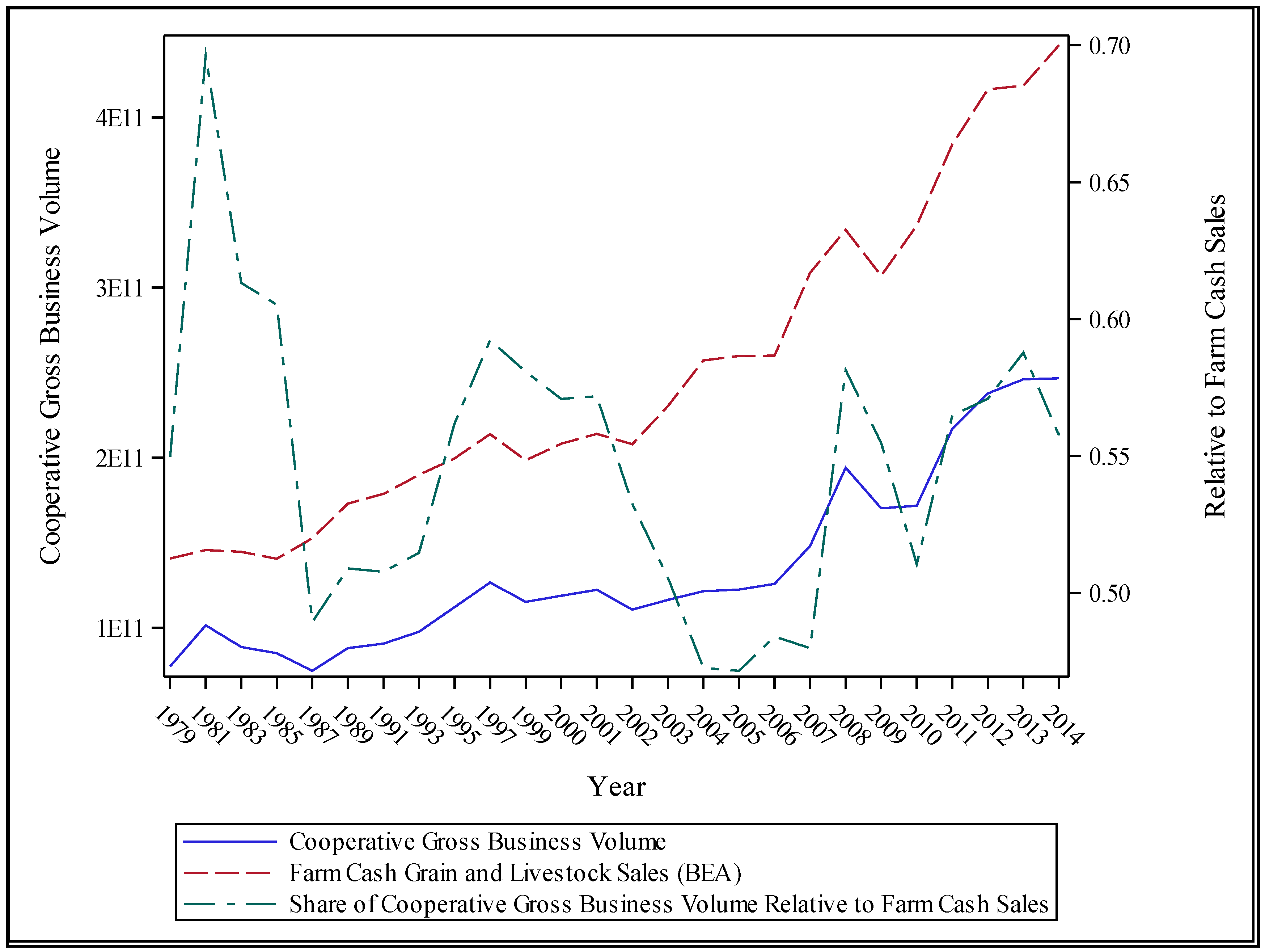
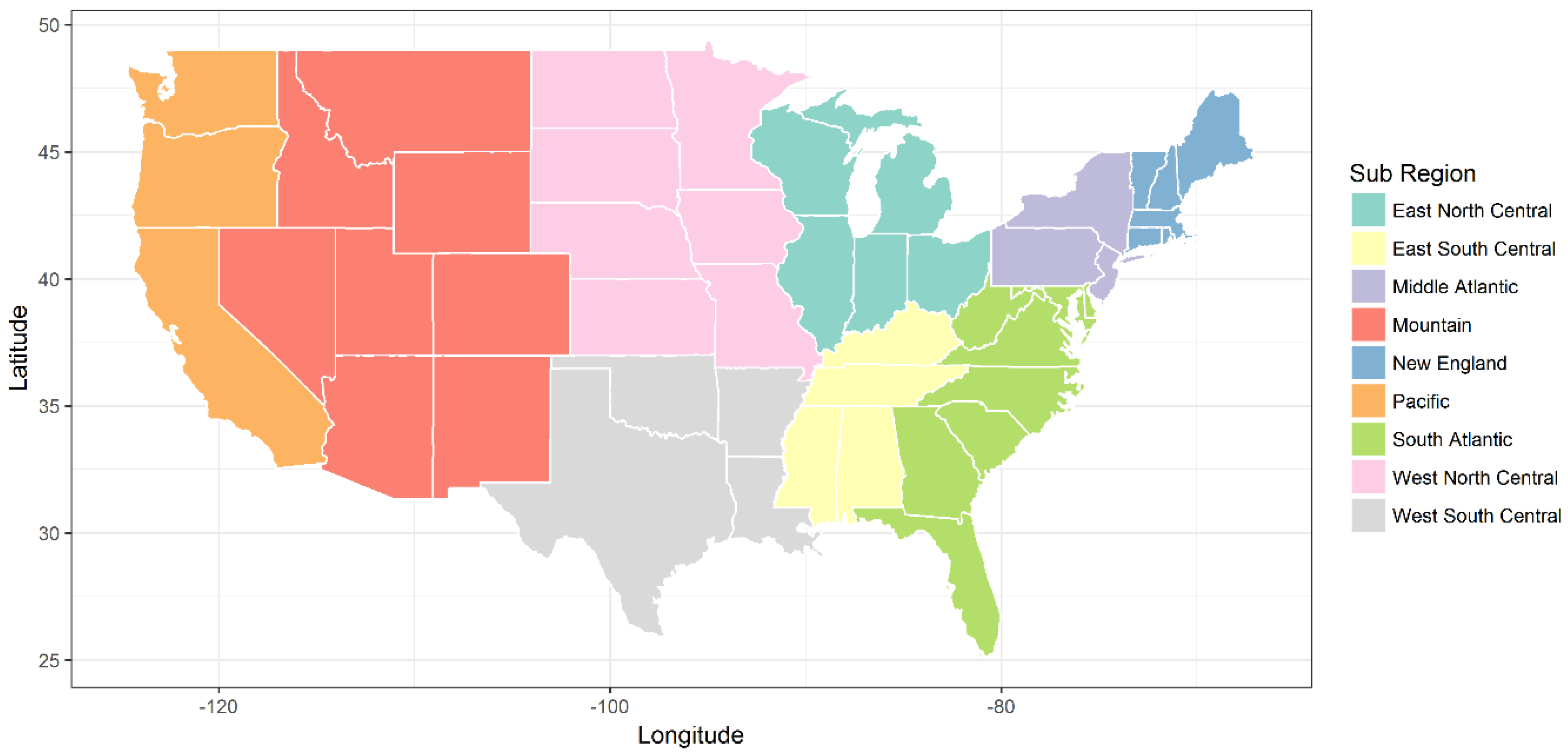
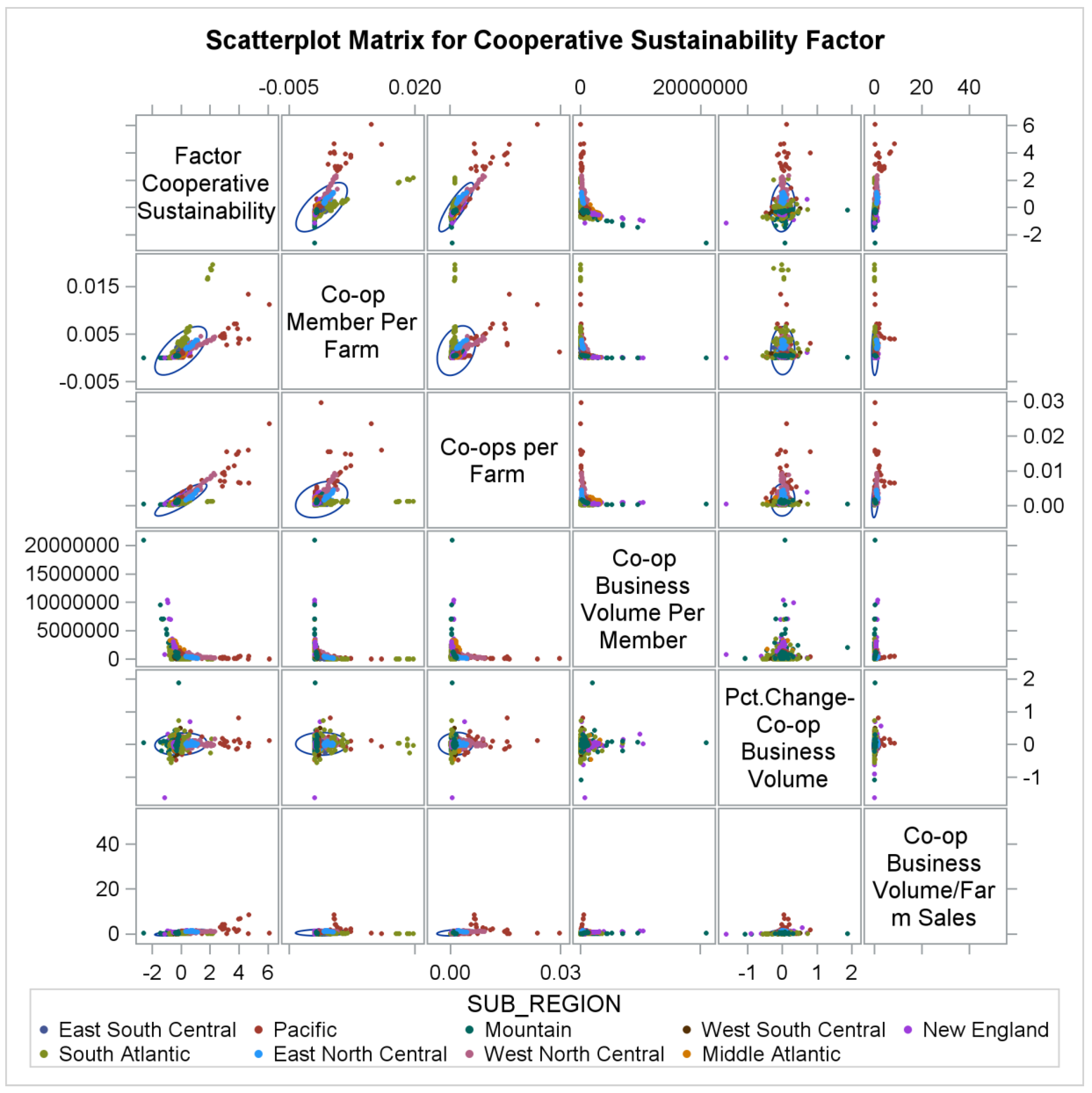
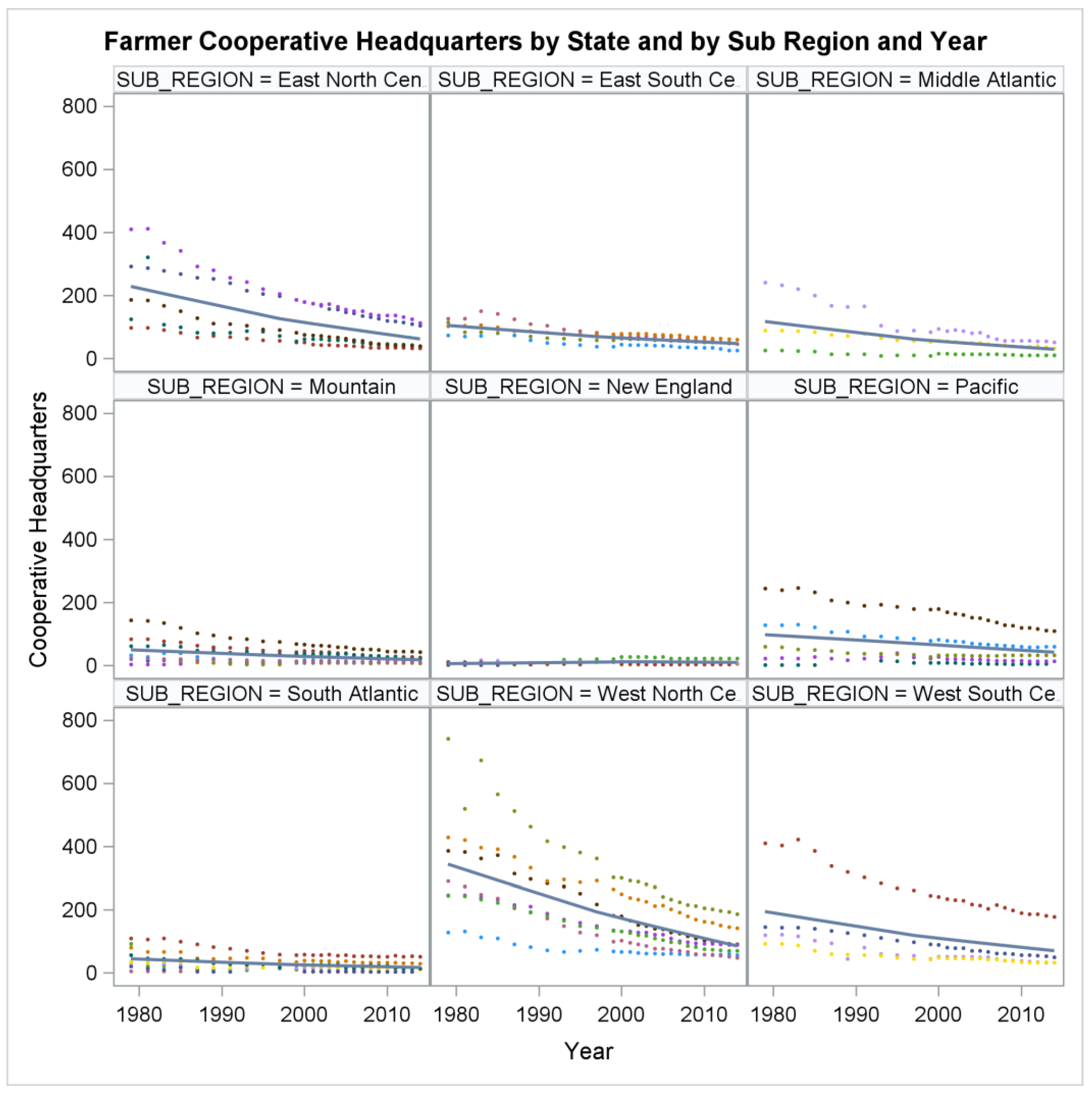
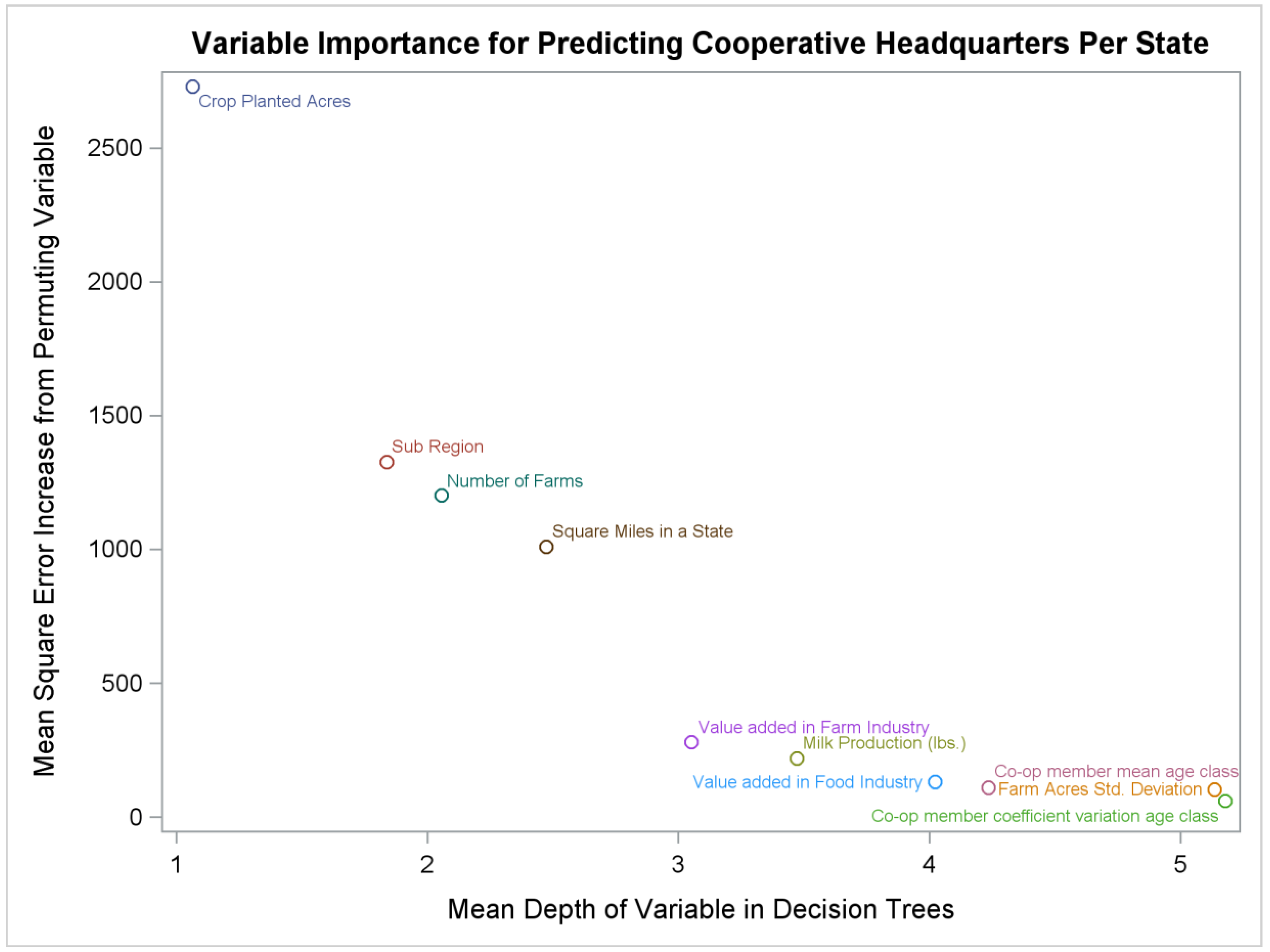
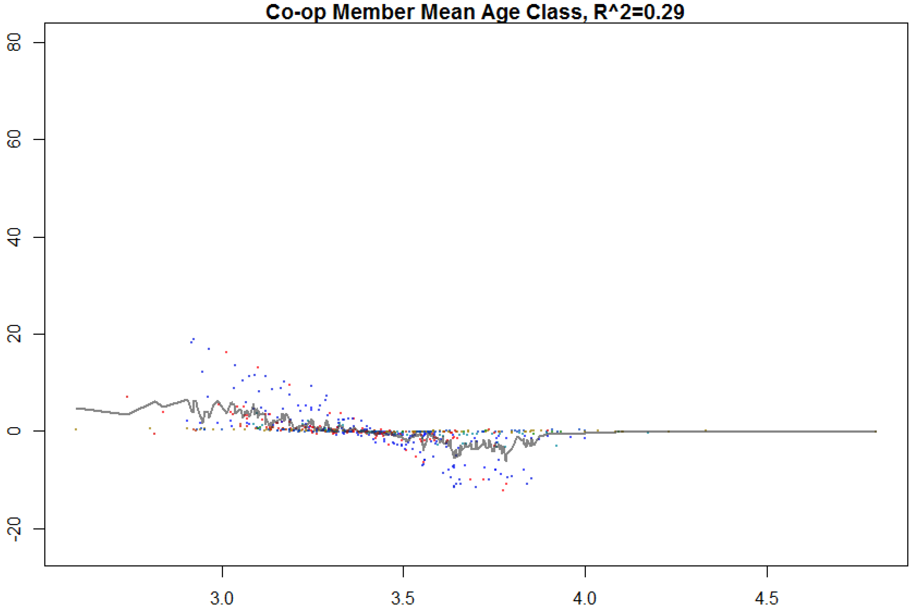
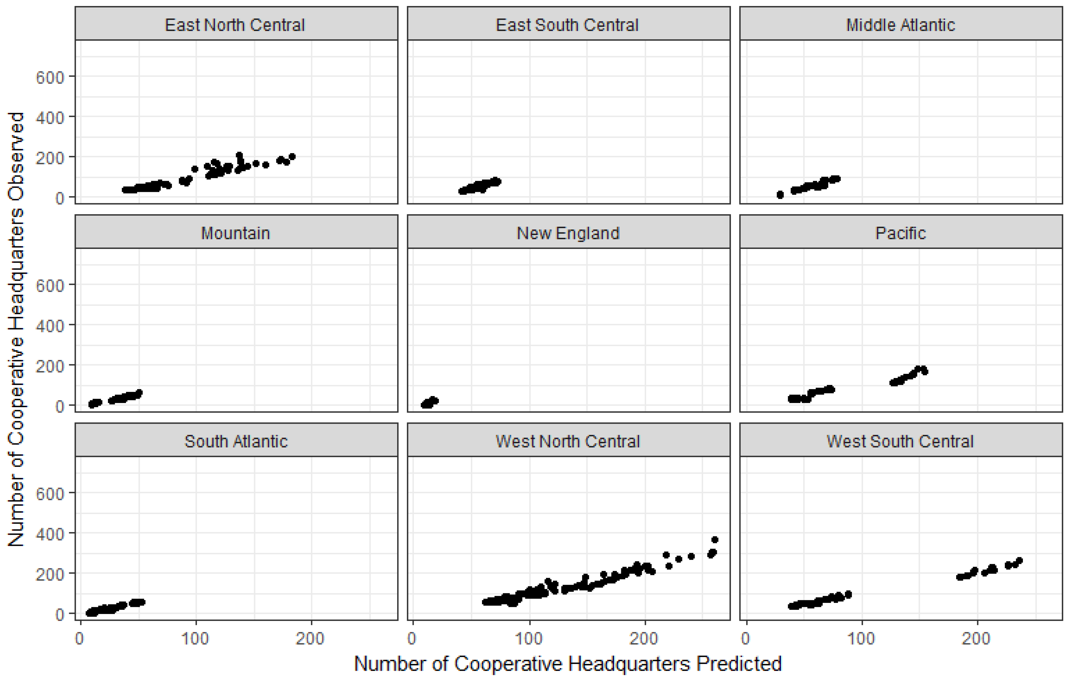
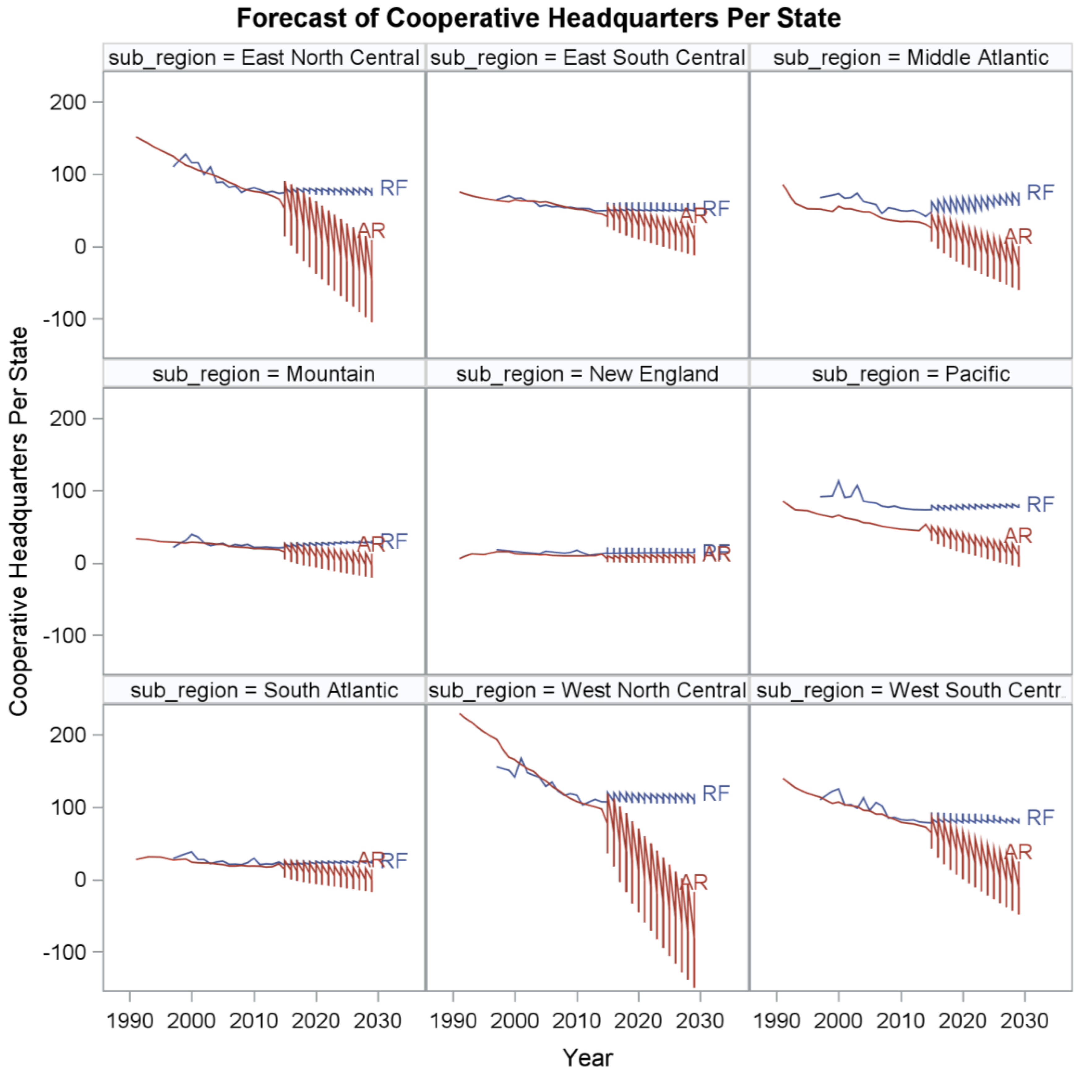
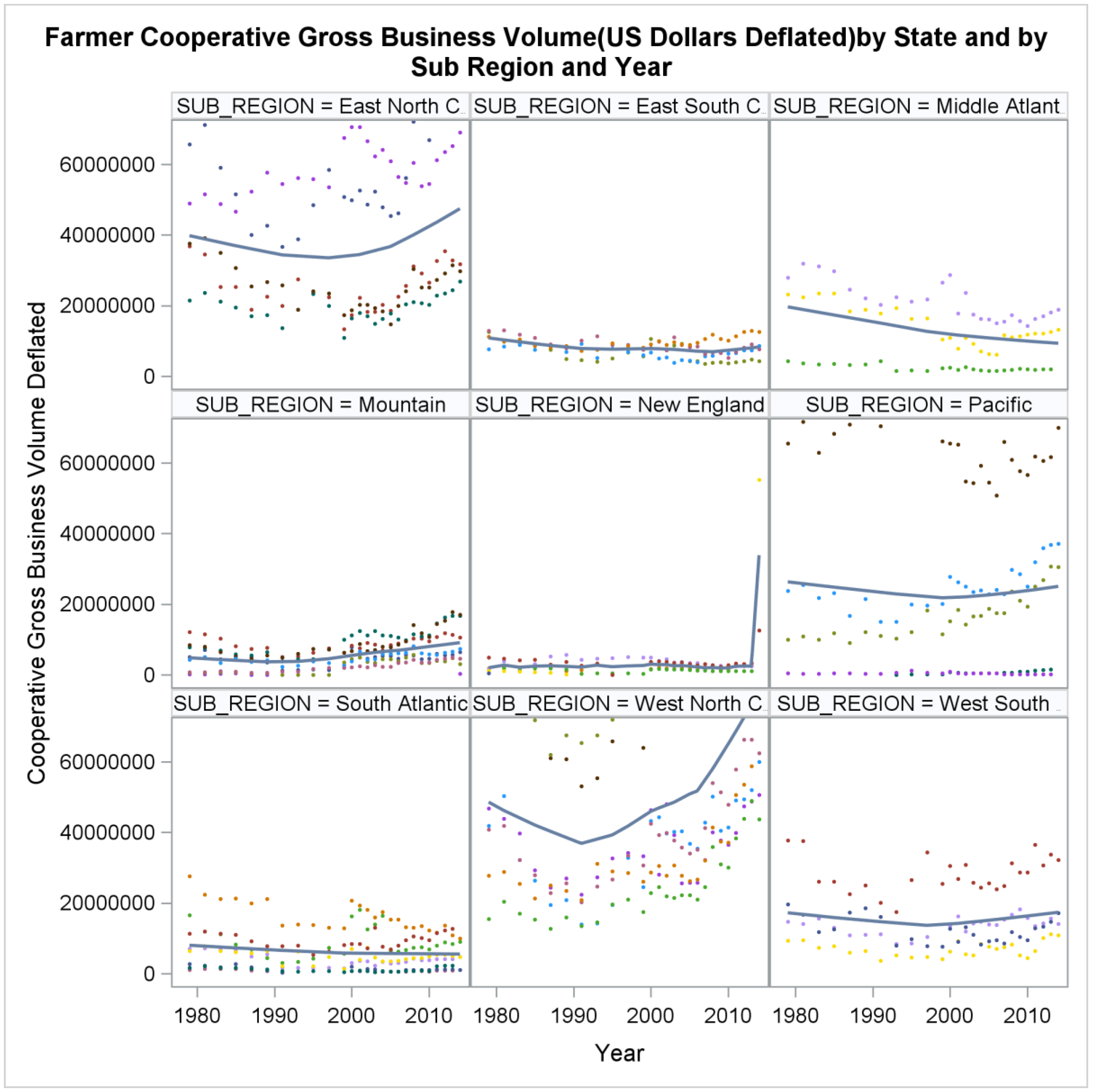
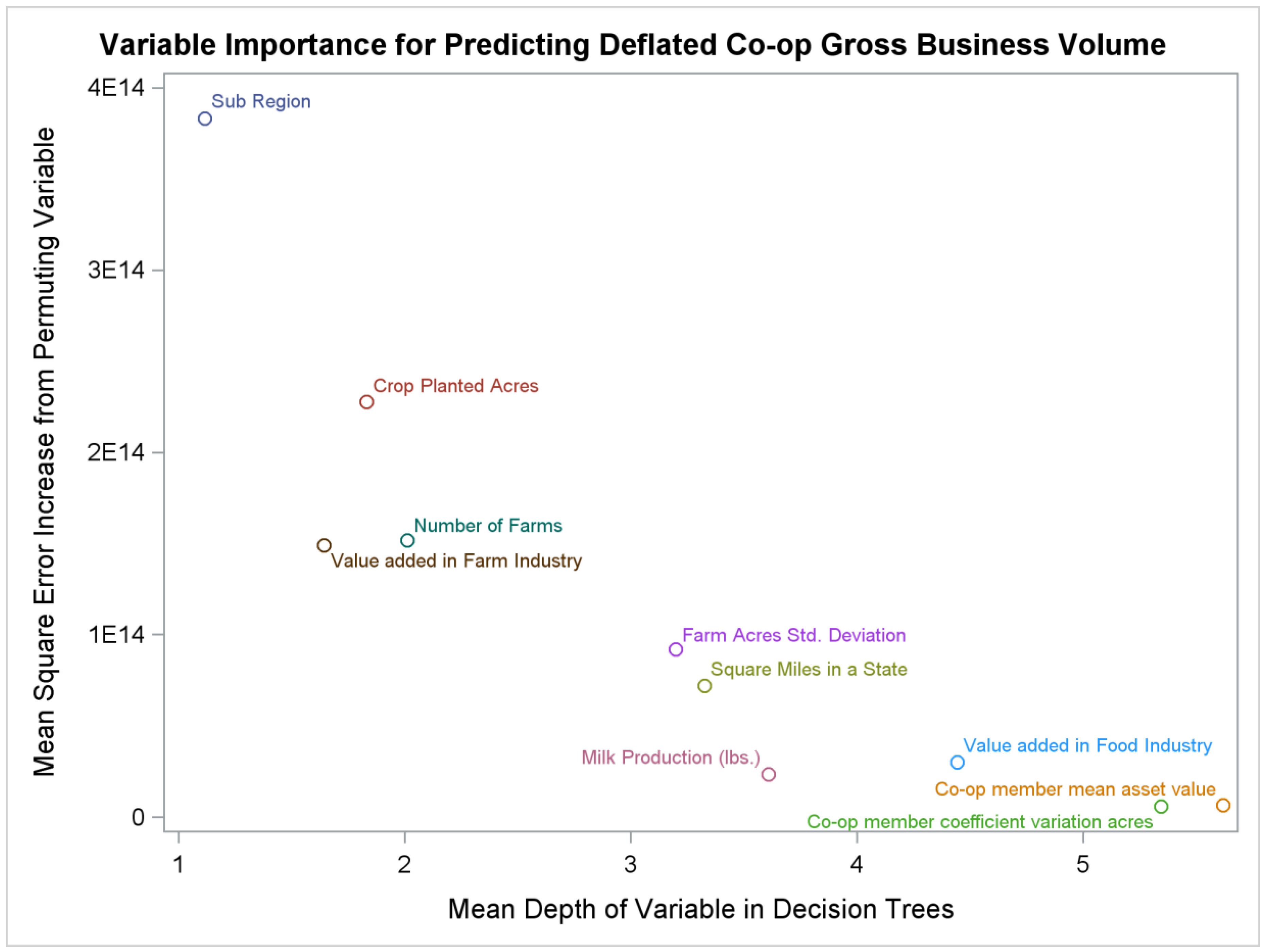
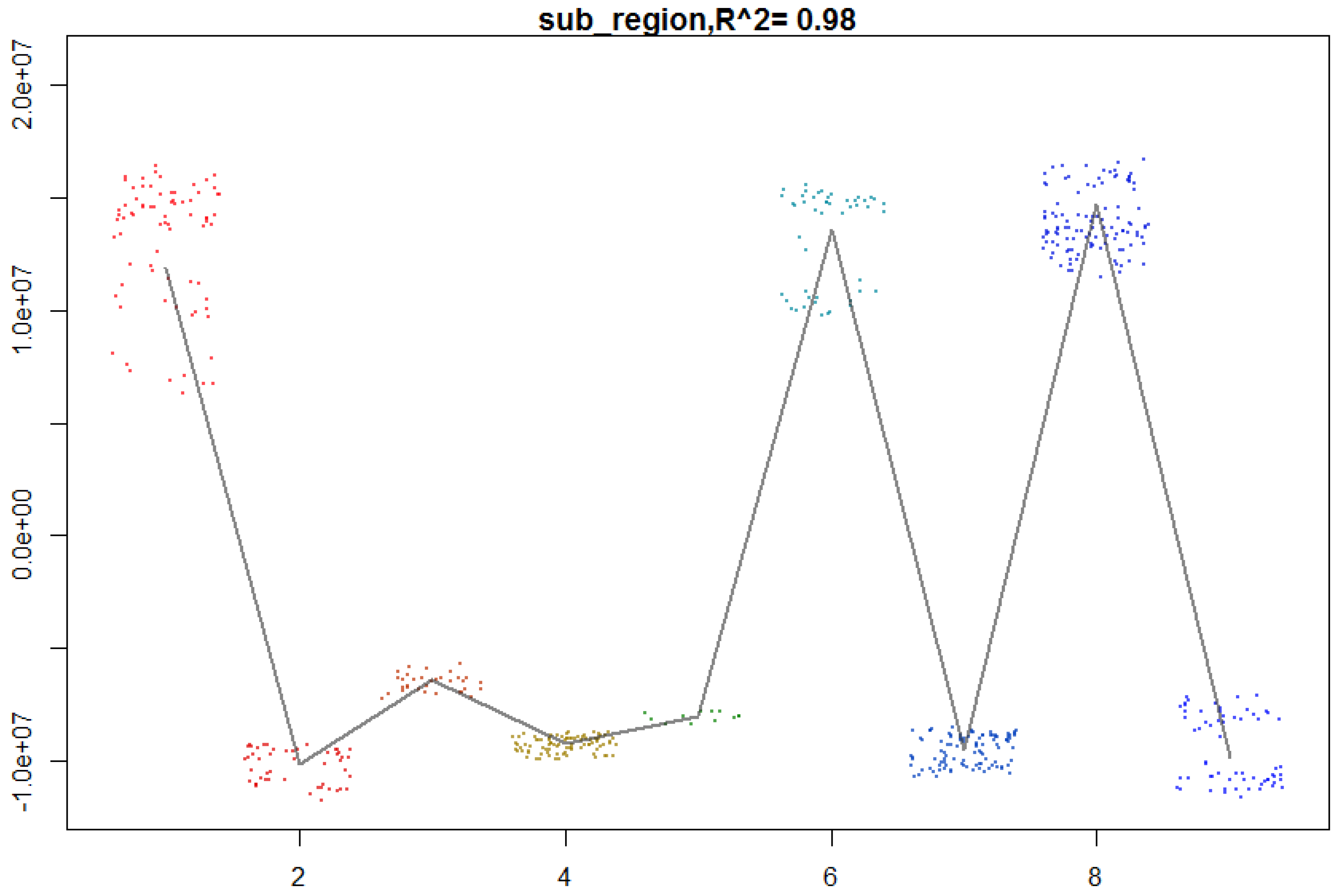
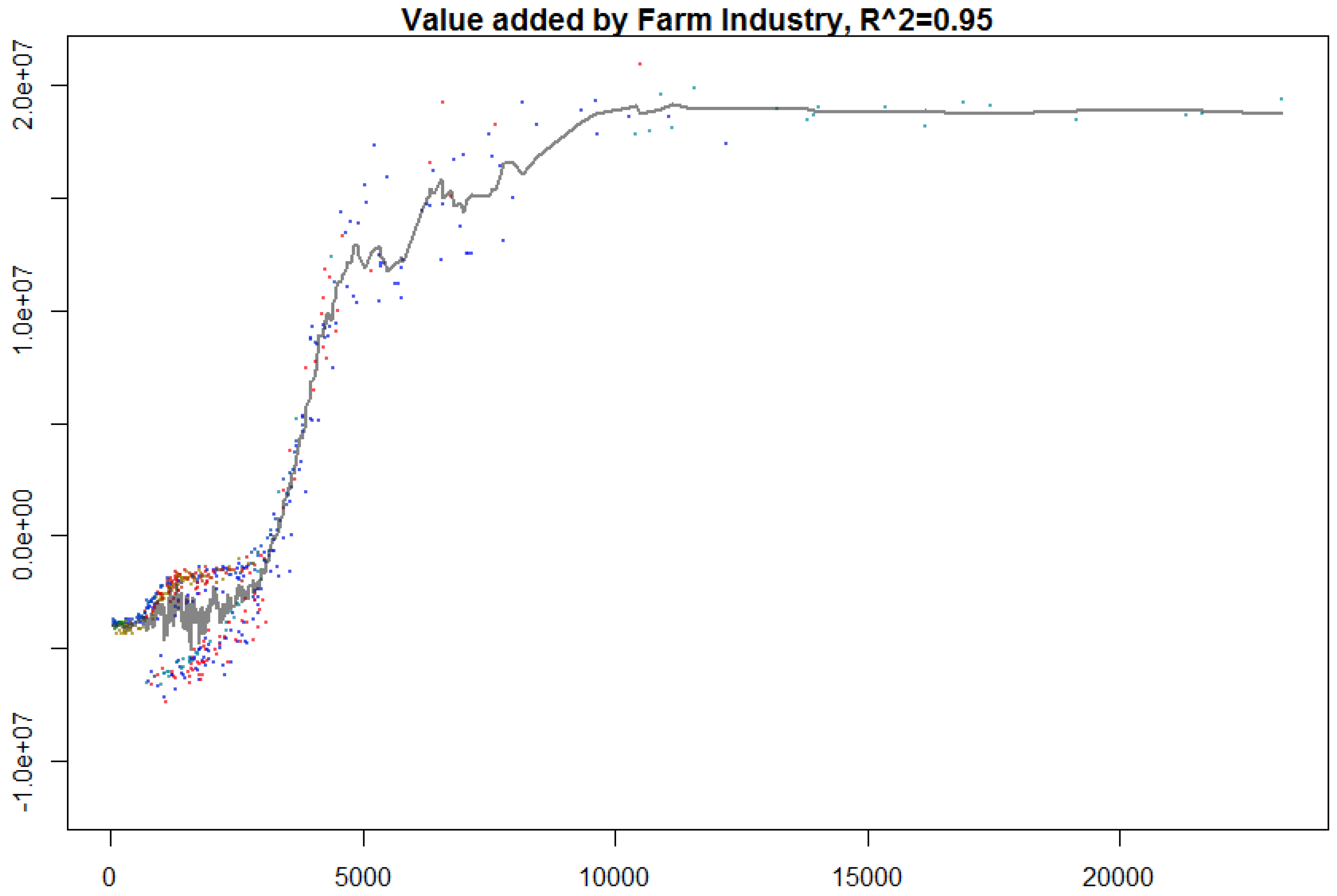
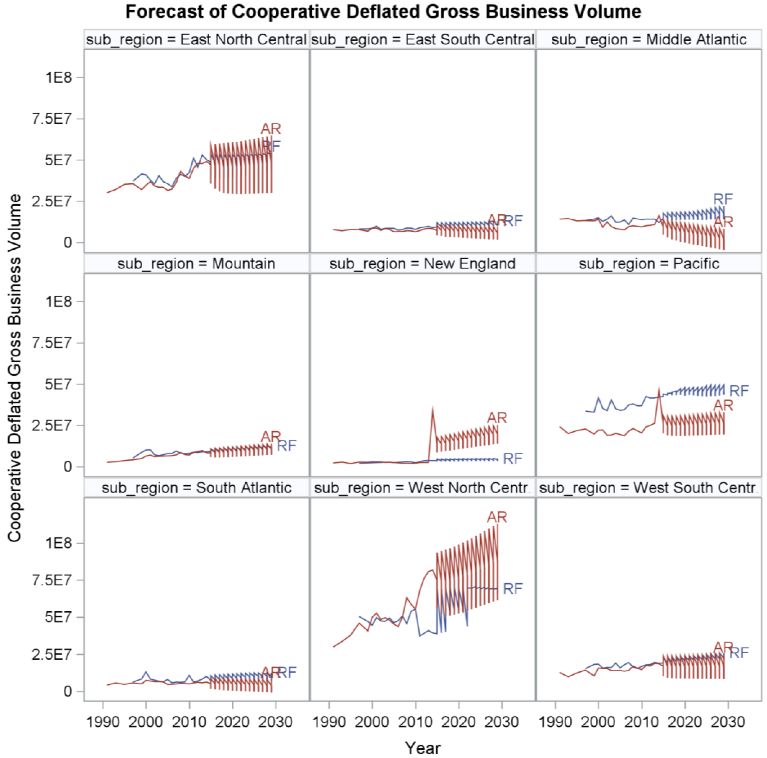
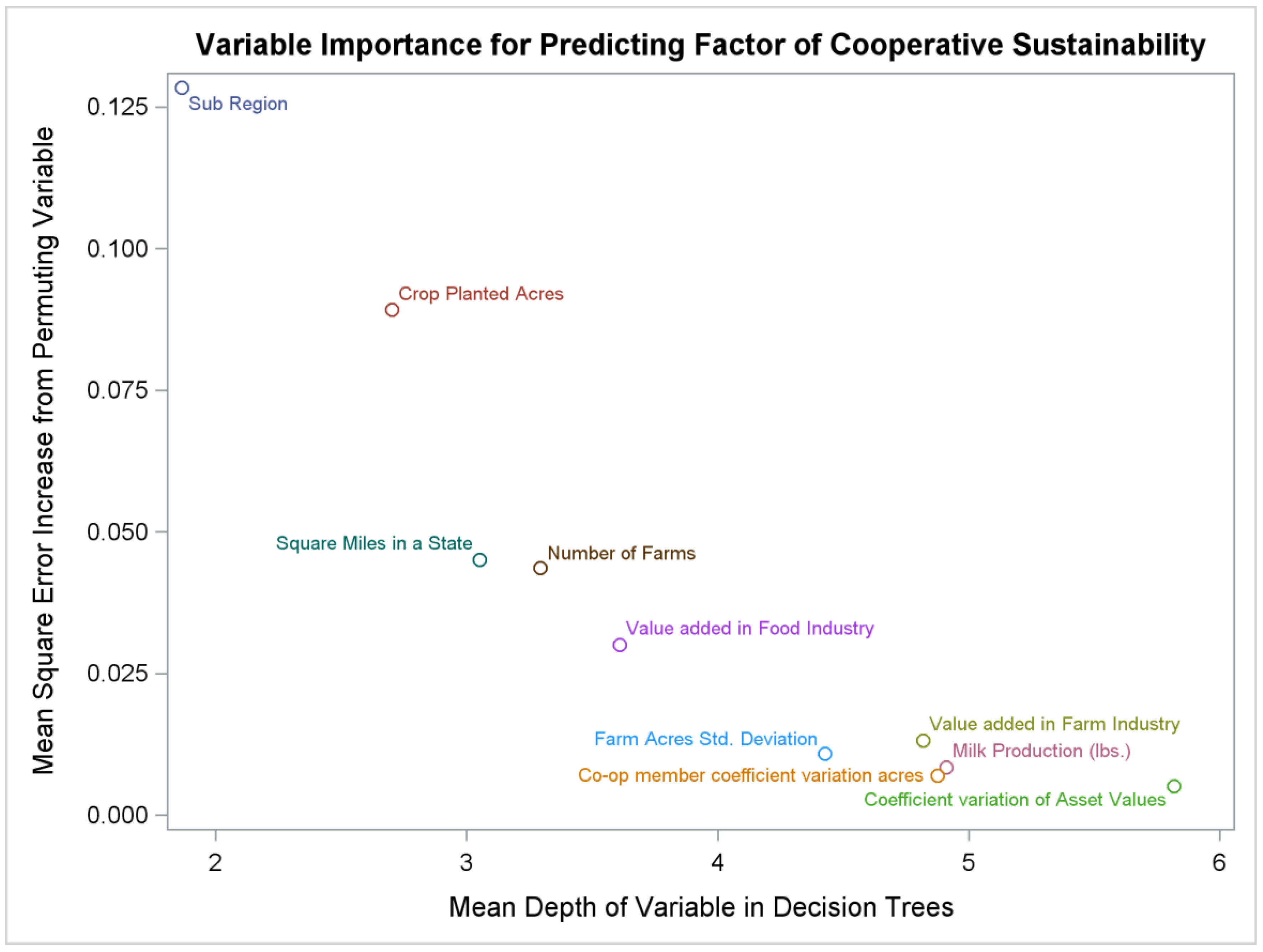
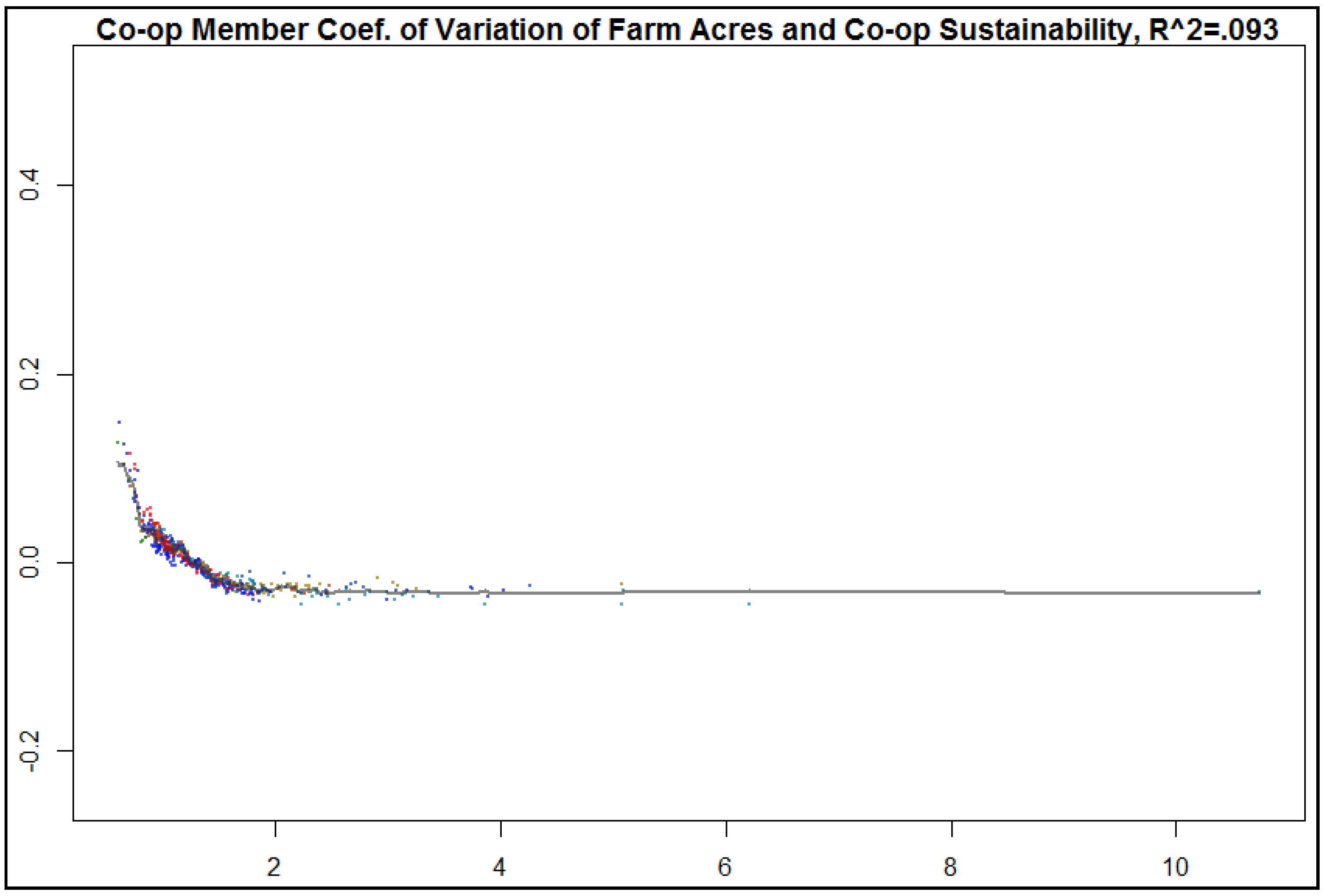
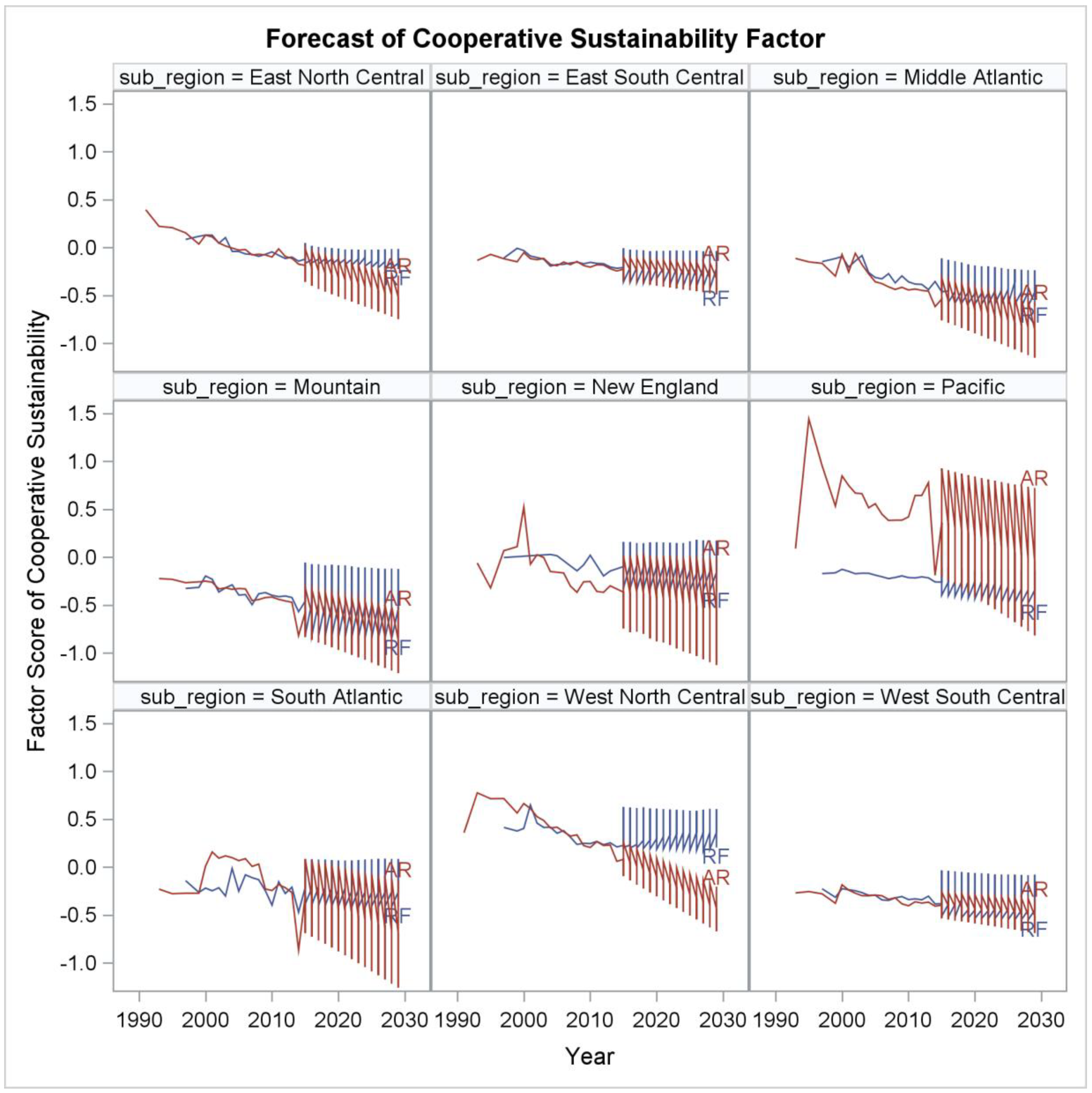
Table 1.
Choices to alter cooperative sustainability, measures of cooperative sustainability, and dimensions of membership heterogeneity expected to affect cooperative sustainability by each approach to cooperative theory.
Table 1.
Choices to alter cooperative sustainability, measures of cooperative sustainability, and dimensions of membership heterogeneity expected to affect cooperative sustainability by each approach to cooperative theory.
| Approach To Cooperative Theory | Cooperative Behavioral Choice That Can Affect Sustainability | Measure of Cooperative Sustainability | Dimensions of Membership Heterogeneity That Affect Cooperative Sustainability |
|---|---|---|---|
| Cooperative as a Firm | Price offered Taxes Membership Inclusion (Open or Closed) | Market Share Member Surplus | Marginal Cost of Production Asset Specificity |
| Cooperative as a Coalition | Governance Rules Coalition Extent Federation | Reduce Externality and Decision-making Costs Maintain Coalition of Members/Farms in a Collective Action Network That Patronize and Participate in the Cooperative Maintain and Return the Collective Good to Members | Socioeconomic Status of Members Age Risk Aversion Farm Size and Specialization |
| Cooperative as a Nexus of Contracts | Discrete Organization Types Contract Parameters | Minimum Organizational Costs Optimal Contract Design Maintain Repeated Contractual Relationships with Members and Employees | Participation Constraints Asset Specificity Risk Aversion Marginal Cost of Production |
Table 2.
Summary statistics for selected variables used in the random forest model.
| Summary Statistics | ||||||
|---|---|---|---|---|---|---|
| Variable | 25th Percentile | Median | 75th Percentile | Mean | Standard Deviation | Median Absolute Difference |
| Number of Cooperatives in a State | 31.0 | 53.0 | 91.0 | 70.9 | 62.7 | 40.0 |
| Cooperative Sustainability Factor | −0.36 | −0.20 | 0.09 | −0.10 | 0.46 | 0.31 |
| State Square Miles | 46,776 | 58,128 | 83,5701 | 71,217 | 45,535 | 26,270 |
| Milk Production (lbs.) | 3.72 × 10⁸ | 1.198 × 10⁹ | 2.51 × 10⁹ | 3.35 × 10⁹ | 6.67 × 10⁹ | 1.33 × 10⁹ |
| Number of Farms | 30,700.0 | 47,600.0 | 75,300.0 | 54,626.0 | 40,242.6 | 29,059.0 |
| Acres Planted to Field Crops | 2,793,000 | 4,873,000 | 13,387,000 | 8,546,532 | 7,706,764 | 5,122,391 |
| Value added by Farm Industry (millions of U.S. dollars) | 1062.0 | 1771.0 | 2988.0 | 2588.1 | 2835.0 | 1298.8 |
| Value added by Food and Kindred Products Industry (millions of U.S. dollars) | 54.0 | 225.0 | 655.0 | 418.3 | 472.9 | 295.0 |
| Ratio of Farm Net Income to Farm Sales | 0.17 | 0.23 | 0.29 | 0.23 | 0.09 | 0.09 |
| Co-op Member Asset Value Coefficient of Variation | 1.00 | 1.18 | 1.47 | 1.31 | 0.55 | 0.32 |
| Co-op Member Mean Asset value (U.S. dollars) | 1,801,958 | 2,598,438 | 3,710,673 | 3,100,767 | 1,935,151 | 1,307,773 |
| Coefficient of Variation to Farm Asset Value (All Farms) | 1.37 | 1.71 | 2.25 | 2.00 | 1.03 | 0.59 |
| Co-op Member Mean Age Class | 3.24 | 3.40 | 3.56 | 3.41 | 0.25 | 0.24 |
| Co-op Member Coefficient of Variation Age Class | 0.29 | 0.32 | 0.35 | 0.32 | 0.04 | 0.04 |
| Co-op Member Socioeconomic Status | −0.49 | −0.17 | 0.31 | 0.01 | 0.74 | 0.57 |
| Co-op Member Socio economic Diversity | −0.14 | 0.03 | 0.21 | 0.01 | 0.33 | 0.26 |
| Co-op Member Farm Type Standard Deviation | 0.43 | 0.47 | 0.49 | 0.45 | 0.06 | 0.04 |
| Farm Acre Standard Deviation (All Farms) | 846.3 | 1502.4 | 3393.8 | 3722.8 | 8070.0 | 1262.8 |
| Co-op Member Coefficient of Variation of Farm Acres | 1.05 | 1.28 | 1.61 | 1.46 | 0.76 | 0.39 |
| Producer Price Index for Food and Feed | 137.3 | 153.8 | 182.3 | 164.9 | 25.9 | 30.7 |
| Farm Producer Price Index | 111.5 | 123.3 | 161.3 | 138.1 | 33.3 | 35.3 |
| Co-op Member Mean Debt (U.S. dollars) | 314,068 | 429,128 | 653,375 | 573,990 | 550,805 | 227,926 |
| Co-op Member Mean Farm Cash Income (U.S. dollars) | 112,138 | 201,447 | 318,538 | 261,292 | 237,436 | 146,578 |
Table 3.
Scoring coefficients for Cooperative Sustainability Factor.
| Standardized Scoring Coefficients for Cooperative Sustainability Factor | ||
|---|---|---|
| Factor 1 | ||
| member_farm | Co-ops Members per Farm | 0.27444 |
| coops_num_farm | Co-ops per Farm | 0.41653 |
| gbv_dfl_member | Co-op Business Volume Per Member | −0.12193 |
| gbv_dfl_chg | Pct. Annual Changes in Co-op Business Volume | 0.03827 |
| coop_mrktshr | Co-op Business Volume/Farm Sales | 0.23504 |
© 2018 by the authors. Licensee MDPI, Basel, Switzerland. This article is an open access article distributed under the terms and conditions of the Creative Commons Attribution (CC BY) license (http://creativecommons.org/licenses/by/4.0/).
Share and Cite
MDPI and ACS Style
Elliott, M.; Elliott, L.; Sluis, E.V.d. A Predictive Analytics Understanding of Cooperative Membership Heterogeneity and Sustainability. Sustainability 2018, 10, 2048. https://doi.org/10.3390/su10062048
AMA Style
Elliott M, Elliott L, Sluis EVd. A Predictive Analytics Understanding of Cooperative Membership Heterogeneity and Sustainability. Sustainability. 2018; 10(6):2048. https://doi.org/10.3390/su10062048
Chicago/Turabian StyleElliott, Matthew, Lisa Elliott, and Evert Van der Sluis. 2018. "A Predictive Analytics Understanding of Cooperative Membership Heterogeneity and Sustainability" Sustainability 10, no. 6: 2048. https://doi.org/10.3390/su10062048
Note that from the first issue of 2016, this journal uses article numbers instead of page numbers. See further details here.