Predicting Coal Consumption in South Africa Based on Linear (Metabolic Grey Model), Nonlinear (Non-Linear Grey Model), and Combined (Metabolic Grey Model-Autoregressive Integrated Moving Average Model) Models

Abstract

South Africa’s coal consumption accounts for 69.6% of the total energy consumption of South Africa, and this represents more than 88% of African coal consumption, taking the first place in Africa. Thus, predicting the coal demand is necessary, in order to ensure the supply and demand balance of energy, reduce carbon emissions and promote a sustainable development of economy and society. In this study, the linear (Metabolic Grey Model), nonlinear (Non-linear Grey Model), and combined (Metabolic Grey Model-Autoregressive Integrated Moving Average Model) models have been applied to forecast South Africa’s coal consumption for the period of 2017–2030, based on the coal consumption in 2000–2016. The mean absolute percentage errors of the three models are respectively 4.9%, 3.8%, and 3.4%. The forecasting results indicate that the future coal consumption of South Africa appears a downward trend in 2017–2030, dropping by 1.9% per year. Analysis results can provide the data support for the formulation of carbon emission and energy policy.

1. Introduction

In recent years, due to the strong relationship between coal consumption and carbon emission, people have paid more attention to coal consumption. However, there are many other factors causing the changes in coal consumption, in addition to the development of modern industry [1]. As the deterioration of global ecological environment, the appeal of reducing carbon emissions is stronger than ever [2,3,4,5]. Peters et al. suggested that the leading cause for current environment problems is the large use of coal by developed countries as well as a few developing countries such as China, as their pursuit of economic growth [6,7]. Therefore, they attribute the responsibility of reducing carbon emission to developed countries and some developing countries [7,8,9]. In fact, in the era of globalization, it is a shared responsibility for all countries to reduce carbon emissions and protect the environment.

Under this special background, it is of great significance to study the coal consumption of South Africa. According to the data in BP Statistical Review of World Energy, South Africa’s main energy sources include coal, oil, etc. In addition, South Africa’s coal consumption makes up 69.6% of the country’s total energy consumption and accounts for 88.7% of African coal consumption, taking the first place in Africa [10]. It illustrates that South Africa is currently excessively dependent on fossil fuel. The government is making efforts to change this situation and planning to improve renewable energy capacity before 2030. Thus, the government intended to spend $50 billion to develop renewable energy and the Renewable Energy Independent Power Producer Procurement Program was launched in 2011, which is a public-private cooperation project, working to achieve South Africa’s transformation to low-carbon economy [11,12]. Not only that, the South African government promised to reduce carbon emission by 34% in 2020 and 42% in 2025 [13]. Therefore, understanding the trend of coal consumption for South African government is important, not only for reducing carbon emissions, but also to ensure the balance of energy supply and demand. More specifically, the long-term prediction for coal consumption will provide data support for the formulation of carbon emission policy, and offer a scientific basis to the transformation of energy in South Africa.

Considering that no studies aimed to straightforwardly forecast coal consumption for South Africa using multiple models at present, the purpose of this study is to strengthen and make up related research, and provide convincing information for policy formulation. We use the mixed models of linear and nonlinear models to forecast South Africa’s coal consumption for the period of 2017–2030. The combination of several models will greatly enhance the reliability of forecasting. The remainder of the study is organized as follows: Section 2 provides a brief literature review, Section 3 introduces the methods and principles of forecasting, Section 4 presents and discusses the forecasting results, and Section 5 provides a summary of this study.

2. Literature Reviews

2.1. Study of Energy Consumption in Other Countries

The literature on energy consumption research has witnessed the emerging studies on coal consumption over the recent years. Some scholars have studied the coal consumption of different countries. For example, Wang et al. used the LMDI (Logarithmic Mean Divisia Index Model) to study the driving factors of China’s coal consumption and provided policy suggestions [7,14]; Apergis et al. made a research on the fluctuations of coal consumption according to the data of all states in America [15]; Gurgul et al. studied the coal consumption’s influence on the economic growth of Portland [16]; besides, India, South Korea, and BRICS also became research focuses in this field [17,18,19,20,21].

2.2. Study of the Energy Consumption in South Africa

In recent years, coal consumption in South Africa has caused much attention and there are many researches centering on it. The present study mainly is focused on the relationship between coal consumption, economic growth, environment, as well as policy implementation on carbon emission reduction. Ziramba adopted the autoregressive distributed lag (ARDL) model to study the long-term relationship and causal relationship between energy consumption, industrial production, and employment in South Africa, and the analysis results showed that industrial production and employment were variables of long-term electric power consumption [22]. While exploring the relationship between South Africa’s coal consumption and carbon emission, Shahbaz et al. also employed the ARDL method and the obtained results showed that economic growth would increase energy emissions; however, financial development would reduce it [23,24]. Through studying the causal relationship among economic growth, pollutant emission, and energy consumption in South Africa, Menyah et al. reported that South Africa can achieve the goal of reducing pollutant emissions by sacrificing economic growth or reducing energy consumption [25]. Al-Mulali et al. studied the effect of energy consumption and carbon emission on economic and financial development of 19 countries (including South Africa) and concluded that carbon emissions were constantly increasing with the high-speed development of national economy and finance [26]. The author suggested that these countries should use energy protection policies to control environmental pollution. Alton et al. advised government to collect carbon taxes from energy consumers, in order to achieve the goal of carbon emission reduction in South Africa until 2025 [27]. Although a great number of researchers are studying coal consumption, the objects are mainly limited to China [7], America, and India. Scholars who study the coal consumption in South Africa mainly focus on the relationship between coal consumption, economy, employment, and pollution. As an obvious result, the economic growth of South Africa will increase energy consumption as well as carbon emissions.

2.3. Study of the Applications of Energy Prediction Models

Energy forecasting models are invented to analyze the future energy development on the basis of available energy information. Their assumption is that some knowledge of the energy development has already existed to reduce energy risk and improve its safety. A large number of energy forecasting models are applied in different situation, where significant achievements have been made. Volkans used the ARIMA (Autoregressive distributed lag Model) to study the energy demand of Turkey [28]; Org used the f-ARIMA model to forecast wind speed [29]; Farahbakhsh applied the residential energy model when studying the residential energy consumption of Canada [30]. Some scholars forecasted the different energy demand based on a single model [31,32,33,34]; Okumus et al. forecasted wind energy power by combining adaptive neural-fuzzy interference system (ANFIS) model with the artificial neural network (ANN), and the obtained error was below 4% while they all exceeded 5% in previous related study [35]. After trying several arithmetic simulations, Yu discovered that Shanghai natural gas short-term load could be forecasted more accurately with relatively less iterations by optimizing Genetic algorithm model (GA Model) and the improving BP neural network [36]. In these researches, combined models are used more often than single models in energy forecasting studies, on account of achieving a higher precision. In addition, different methods apply to forecasting of different requirement and content, and we need to select the most suitable forecasting model, according to the practical situation.

As stated above, researchers have noticed the importance of coal consumption of South Africa [27,37]. However, there are no studies related to coal consumption forecasting of South Africa To improve the accuracy of the prediction, this paper using a combined method of linear and nonlinear models to forecast the coal consumption. In this study, Metabolic Grey Model (MGM), Non-linear Grey Model (NGM), and Metabolic Grey Model-Autoregressive Integrated Moving Average Model (MGM-ARIMA) combined models are used to forecast South Africa’s coal consumption in 2017–2030.

3. Methodology

3.1. The Non-Linear Grey Model

The NGM is a model based on improvement of the gray model [38]. The core of traditional gray model is a first order differential equation. In addition, the forecasting data obtained by this method always presents a linear tendency, which greatly narrows the application scope of this model. The NGM has added a power coefficient to the core differential equation, thus enabling the forecasting value to show nonlinear characteristics. The specific operation steps are shown in the following:

First, we give the first five values of the original data and name the sequence: $X^{\left(0\right)}$. Then, according to accumulative principle, the original sequence can be processed into an accumulative sequence: $X^{\left(1\right)}$

$$X^{\left(0\right)}=\left(x^{\left(0\right)}\left(i+1\right),x^{\left(0\right)}\left(i+2\right),x^{\left(0\right)}\left(i+3\right),x^{\left(0\right)}\left(i+4\right),x^{\left(0\right)}\left(i+5\right)\right)\left(i=0,1,\cdots n-6\right)$$

(1)

$$X^{\left(1\right)}=\left\{x^{\left(1\right)}\left(1\right),x^{\left(1\right)}\left(2\right),\dots ,x^{\left(1\right)}\left(n\right)\right\}$$

(2)

For the convenience of operation, we need to define an auxiliary sequence: $Z^{\left(1\right)}\left(k\right)$, by adding and subtracting the accumulative sequence.

$$Z^{\left(1\right)}\left(k\right)=0.5x^{\left(1\right)}\left(k\right)+0.5x^{\left(1\right)}\left(k-1\right)$$

(3)

Based on this, the core equation of the NGM can be obtained, as shown in Equation (4). We use the least square method to solve the coefficients ‘a’ and ‘b’. Then, the solution of Equation (5) can be obtained.

$$x^{\left(0\right)}\left(k\right)+a{(Z^{\left(1\right)}\left(k\right))}^{\alpha }=b$$

(4)

Here, ‘a’ and ‘b’ represent the coefficients of differential equation, ‘$\alpha$’ represents power coefficient.

$$\frac{d{x}^{\left(1\right)}\left(t\right)}{dt}+a{(x^{\left(1\right)}\left(t\right))}^{\alpha }=b$$

(5)

The principle of least square method is shown in Equations (6)–(8).

$${\left[a,b\right]}^T={\left(B^{T}B\right)}^{-1}{B}^T{Y}_N$$

(6)

$$Y_N={\left[x^{\left(0\right)}\left(2\right),\dots ,x^{\left(0\right)}\left(n\right)\right]}^T$$

(7)

$$B=\left[\begin{array}{c}\begin{array}{cc}-Z^{\left(1\right)}{\left(2\right)}^{\alpha }& 1\\ -Z^{\left(1\right)}{\left(3\right)}^{\alpha }& 1\end{array}\\ \begin{array}{cc}⋮& ⋮\\ -Z^{\left(1\right)}{\left(n\right)}^{\alpha }& 1\end{array}\end{array}\right]$$

(8)

Then introduce the known parameter value into Equation (4) and combine solution Equations (9) and (10) of four-order Lingo. Finally, the final forecasting value will be obtained by subtraction.

$$\frac{dX}{dt}=F\left(t,X\right)$$

(9)

$$\{\begin{array}{c}\begin{array}{c}{K}_1=F\left(t_n,X_n\right)\\ K_2=F\left(t_n+\frac{h}{2},X_n+\frac{h}{2}{K}_1\right)\\ K_3=F\left(t_n+\frac{h}{2},X_n+\frac{h}{2}{K}_2\right)\end{array}\\ K_4=F\left(t_n+h,X_n+h{K}_3\right)\\ X_{n+1}=X_n+\frac{h}{6}\left[K_1+2K_2+2K_3+K_4\right]\end{array}$$

(10)

$${\widehat{x}}^{\left(0\right)}\left(k+1\right)={\widehat{x}}^{\left(1\right)}\left(k+1\right)-{\widehat{x}}^{\left(1\right)}\left(k\right)$$

(11)

3.2. The Metabolic Grey Model

The MGM is different from NGM, which has no power coefficient and the specific form is shown in Equation (12). Through differentiation processing, its solution is presented in Equation (14).

$$x^{\left(0\right)}\left(k\right)+a{Z}^{\left(1\right)}\left(k\right)=b$$

(12)

$$\frac{d{x}^1}{dt}+a{x}^1=b$$

(13)

$${\widehat{x}}_{k+1}^1=\left(x_1^0-\frac{b}{a}\right)e^{-ak}+\frac{b}{a},k=\left(1,2,\cdots ,m\right)$$

(14)

Here, ‘a’ and ‘b’ represent the coefficients of differential equation, and the unknown parameter can be obtained according to the solution of the following matrix. Finally, the expression of the unknown value is in Equation (17).

$${\left[a,b\right]}^T={\left(B^{T}B\right)}^{-1}{B}^{T}Y$$

(15)

$$B=\left(\begin{array}{cc}-\left(x_1^1+x_2^1\right)/2& 1\\ ⋮& ⋮\\ -\left(x_{m-1}^1+x_m^1\right)/2& 1\end{array}\right),Y=\left(\begin{array}{c}{x}_2^0\\ ⋮\\ x_m^0\end{array}\right)$$

(16)

$${\widehat{x}}_{k+1}^0={\widehat{x}}_{k+1}^1-{\widehat{x}}_k^1=\left(1-e^a\right)\left({\widehat{x}}_1^0-\frac{b}{a}\right)e^{-ak},k=\left(1,2,\cdots ,m\right)$$

(17)

This is the complete calculation process. The MGM is composed of complete operation and continuous cycle. Every time finishing the calculating operation, the earliest data will be removed, and the new data reflecting system characteristics is added. Every step is operated according to this procedure.

3.3. The Metabolic Grey Model-Autoregressive Integrated Moving Average Model

Five data points are selected to forecast the sixed data point, which is called a cycle process [39]. In this study, the first 5-year data sequence is used as an example. In the next forecasting cycle, we added one new data point and removed one old data point to ensure that the forecasting data size of every step is five [40].

For each cycle process, the cut data sequence is recorded as:

$$X^{\left(0\right)}=\left\{x^{\left(0\right)}\left(1\right),x^{\left(0\right)}\left(2\right),\dots ,x^{\left(0\right)}\left(n\right)\right\}$$

(18)

To forecast the (n + 1)th data, a differential equation is used for the auxiliary calculation and the specific steps are as follows [41]:

An accumulative sequence is defined as $X^{\left(1\right)}=\left\{x^{\left(1\right)}\left(1\right),x^{\left(1\right)}\left(2\right),\dots ,x^{\left(1\right)}\left(n\right)\right\}$.

Where $x^{\left(1\right)}\left(k\right)={{\displaystyle \sum }}_{i=1}^k{x}^{\left(0\right)}\left(i\right),k=1,2,3,\dots ,n$. Then establish the differential equation of sequence $X^{\left(1\right)}$: $\frac{d{x}^{\left(1\right)}}{dt}+a{x}^{\left(1\right)}=b$. As long as parameters ‘a’ and ‘b’ can be solved, the solution of sequence $X^{\left(1\right)}$ can be obtained.

To solve this differential equation, the following auxiliary sequence is introduced: $Z^{\left(1\right)}\left(k\right)=0.5x^{\left(1\right)}\left(k\right)+0.5x^{\left(1\right)}\left(k-1\right)$.

By using the least square method, we can obtain: ${\left[a,b\right]}^T={\left(B^{T}B\right)}^{-1}{B}^{T}Y$.

Where:

$$Y_N={\left[x^{\left(0\right)}\left(2\right),x^{\left(0\right)}\left(3\right),\dots ,x^{\left(0\right)}\left(n\right)\right]}^T$$

(19)

$$B=\left[\begin{array}{c}\begin{array}{cc}-Z^{\left(1\right)}\left(2\right)& 1\\ -Z^{\left(1\right)}\left(3\right)& 1\end{array}\\ \begin{array}{cc}⋮& ⋮\\ -Z^{\left(1\right)}\left(n\right)& 1\end{array}\end{array}\right]=\left[\begin{array}{c}\begin{array}{cc}-\left(0.5x^{\left(1\right)}\left(2\right)+0.5x^{\left(1\right)}\left(1\right)\right)& 1\\ -\left(0.5x^{\left(1\right)}\left(3\right)+0.5x^{\left(1\right)}\left(2\right)\right)& 1\\ ⋮& ⋮\\ -\left(0.5x^{\left(1\right)}\left(n\right)+0.5x^{\left(1\right)}\left(n-1\right)\right)& 1\end{array}\end{array}\right]$$

(20)

Then, the parameters ‘a’ and ‘b’ can be acquired and the solution of sequence $X^{\left(1\right)}$ is:

$${\widehat{x}}^{\left(1\right)}\left(k\right)=\left[x^{\left(0\right)}\left(1\right)-\frac{b}{a}\right]e^{-a\left(k-1\right)}+\frac{b}{a},k=1,2,\dots ,n$$

(21)

$${\widehat{x}}^{\left(0\right)}\left(k\right)={\widehat{x}}^{\left(1\right)}\left(k\right)-{\widehat{x}}^{\left(1\right)}\left(k-1\right)=\left[x^{\left(0\right)}\left(1\right)-\frac{b}{a}\right]\left(1-e^a\right)e^{-a\left(k-1\right)},k=2,3,\dots ,n$$

(22)

The next step is correcting the residual error by the ARIMA model. The ARIMA model is composed of three parts: error stabilization, moving average process, and autoregressive process [42]. These three processes correspond to Equations (5)–(7), respectively.

$$Y_t^{*}={\left(1-B\right)}^d{Y}_t$$

(23)

$$Y_t^{*}=c+{\alpha }_1{Y}_{t-1}+{\alpha }_2{Y}_{t-2}+\cdots +{\alpha }_p{Y}_{t-p}+u_t$$

(24)

$$Y_t^{*}=u_t+{\beta }_1{u}_{t-1}+{\beta }_2{u}_{t-2}+\cdots +{\beta }_q{u}_{t-q}$$

(25)

Thus, the complete formula of the ARIMA model is as follows:

$$Y_t^{*}=\mathrm{c}+{\alpha }_1{Y}_{t-1}+{\alpha }_2{Y}_{t-2}+\cdots +{\alpha }_k{Y}_{t-k}+{\mu }_t+{\beta }_1{\mu }_{t-1}+{\beta }_2{\mu }_{t-2}+\cdots +{\beta }_q{\mu }_{t-q}$$

(26)

Here, $Y_t$ represents the original sequence; $Y_t^{*}$ represents the stationary sequence after d-order difference; d represents the order of difference; c represents the constant variable; ${\alpha }_{\mathrm{i}}$ and ${\beta }_{\mathrm{i}}$ represent parameters; $u_t$ represents error term.

This study selected the MGM, NGM, and the MGM-ARIMA model to predict the energy consumption of South Africa. Each model has its own advantages and disadvantages. The grey model is good at describing the laws of a fuzzy system with very little information. However, the required precision can be achieved only for the first 1–2 data points of the forecast. Based on the traditional grey model, the MGM increases the running cycles and ensures the accuracy of each predicted value. However, its forecasting result cannot reflect the nonlinearity of original data series. The NGM can exhibit nonlinear traits and guarantee the update of forecasting data [43], while its calculation process is relatively complex. The MGM-ARIMA model we have established not only inherits all the advantages of the MGM model but it also has its own special advantages. The addition of ARIMA further improves the accuracy of forecasting results.

4. Empirical Results and Discussion

4.1. Display of Data

All data sources for the study are obtained from BP Statistical Review of World Energy [44]. Based on the coal consumption of South Africa during the period of 2000–2016 (as shown in Appendix A

Table A1. Coal consumption in South Africa 2000–2016 (Unit: Mtoe).

YEAR	2000	2001	2002	2003	2004	2005
Coal Consumption	74.631	74.898	71.247	79.189	86.767	79.988
YEAR	2006	2007	2008	2009	2010	2011
Coal Consumption	81.473	83.661	93.336	93.824	92.823	90.512
YEAR	2012	2013	2014	2015	2016
Coal Consumption	88.339	88.613	89.839	83.350	85.108

), we establish MGM, NGM, and MGM-ARIMA models to forecast the coal consumption of South Africa for 2017–2030.

During the calculating process of the three models, the entire stage can be mainly divided into two parts: fitting and forecasting. In the fitting process, the known data is calculated following the forecasting steps. Through comparing the known data with fitting results, the accuracy of the forecasting model can be judged. The forecasting process outputs the forecasting results of unknown data. By analyzing the tendency of forecasting results, we can judge the variations of coal consumption in South Africa.

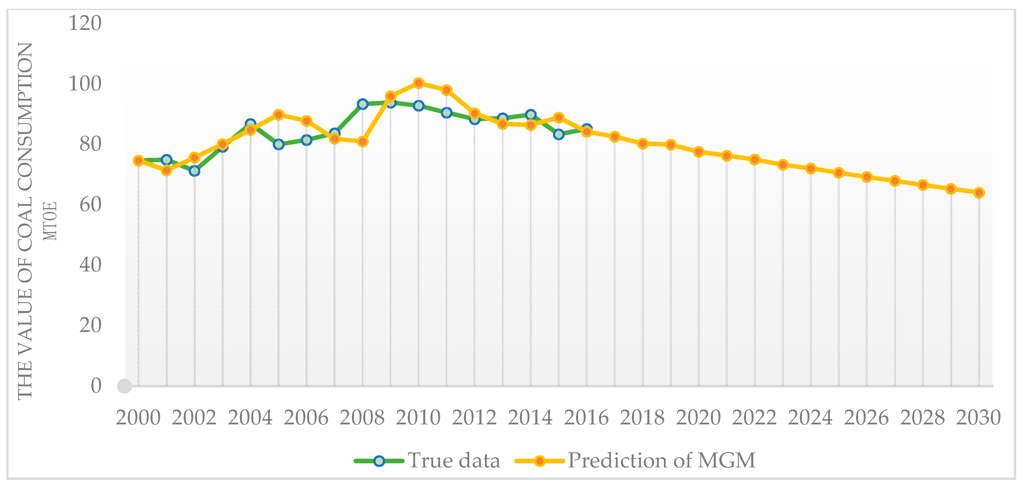
4.2. Calculation Process of the MGM Model

During calculation process of MGM, old elements are removed and new elements are added. The data reflecting the system real-time characteristic is adopted for forecasting. As shown in this study, we selected five-dimensional data as the basis of modeling. For example, in the initial cycle, five-year data in 2000–2004 is used to forecast the value in 2005. We can get a series of gray differential equation coefficients via calculation. Figure 1 below shows the parameter values obtained from these cycle processes.

With the parameters in Figure 1, the final forecasting result of this model can be calculated through the formula of solving differential equation. By applying the least square method, the forecasting result of the MGM is shown in Figure 2.

As illustrated in Figure 2, the green line represents the original data of South Africa’s coal consumption, and the yellow line represents the forecasting coal consumption in 2000–2030. It shows that although the original data of 2000–2016 is slightly different from the forecasting value during the fitting stage, their overall tendency is identical. During the forecasting stage, we can see that the coal consumption calculated by the MGM is decreasing in 2017–2030.

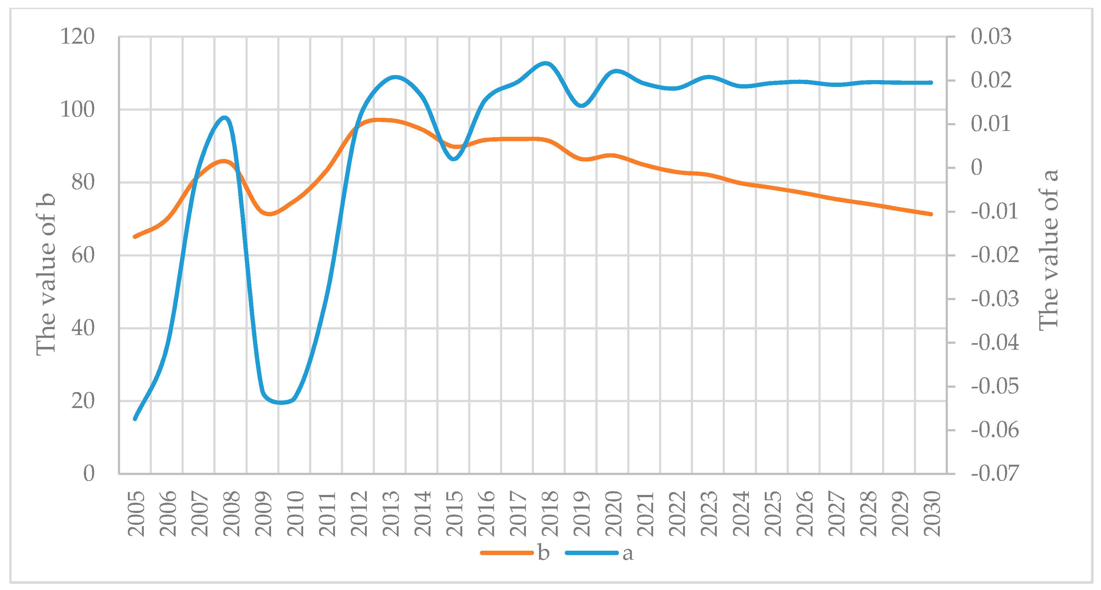
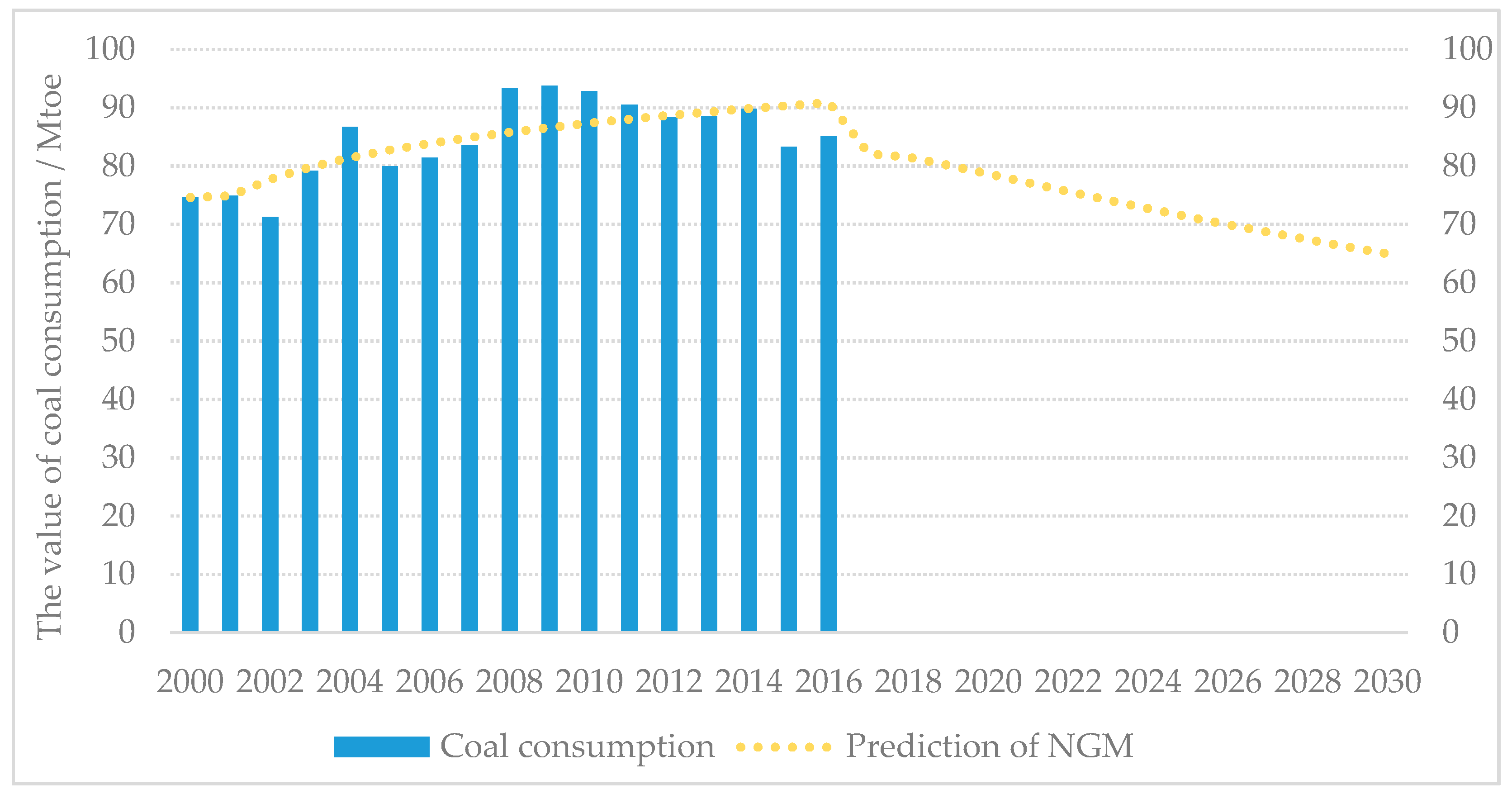
4.3. Calculation Process of the NGM Model

In NGM model, the element of power coefficient is added to the differential equation of the traditional gray model. With the help of Matlab software, the power coefficient can be easily calculated, which is shown in

Table 1. Power coefficient of the NGM model.

YEAR	2004	2005	2006	2007	2008	2009	2010
The Power Coefficient	1	0.842	0.001	0.001	1	1	0.001
YEAR	2011	2012	2013	2014	2015	2016
The Power Coefficient	1	1	0.913	0.001	1	1

Note: The Power coefficient ‘$\mathsf{\alpha }$’ corresponds to Equation (5).

.

On this basis, the final forecasting value of NGM is shown in Figure 3. It can be seen obviously that the tendency of the results in forecasting stage is consistent with the metabolic gray model, which are both decreasing. To judge the goodness of fit, in Figure 3, the blue columns represent the original value of coal consumption, while the yellow line indicates the forecasting value obtained by the NGM. Obviously, the data’s tendency during fit stage is roughly consistent with the original data.

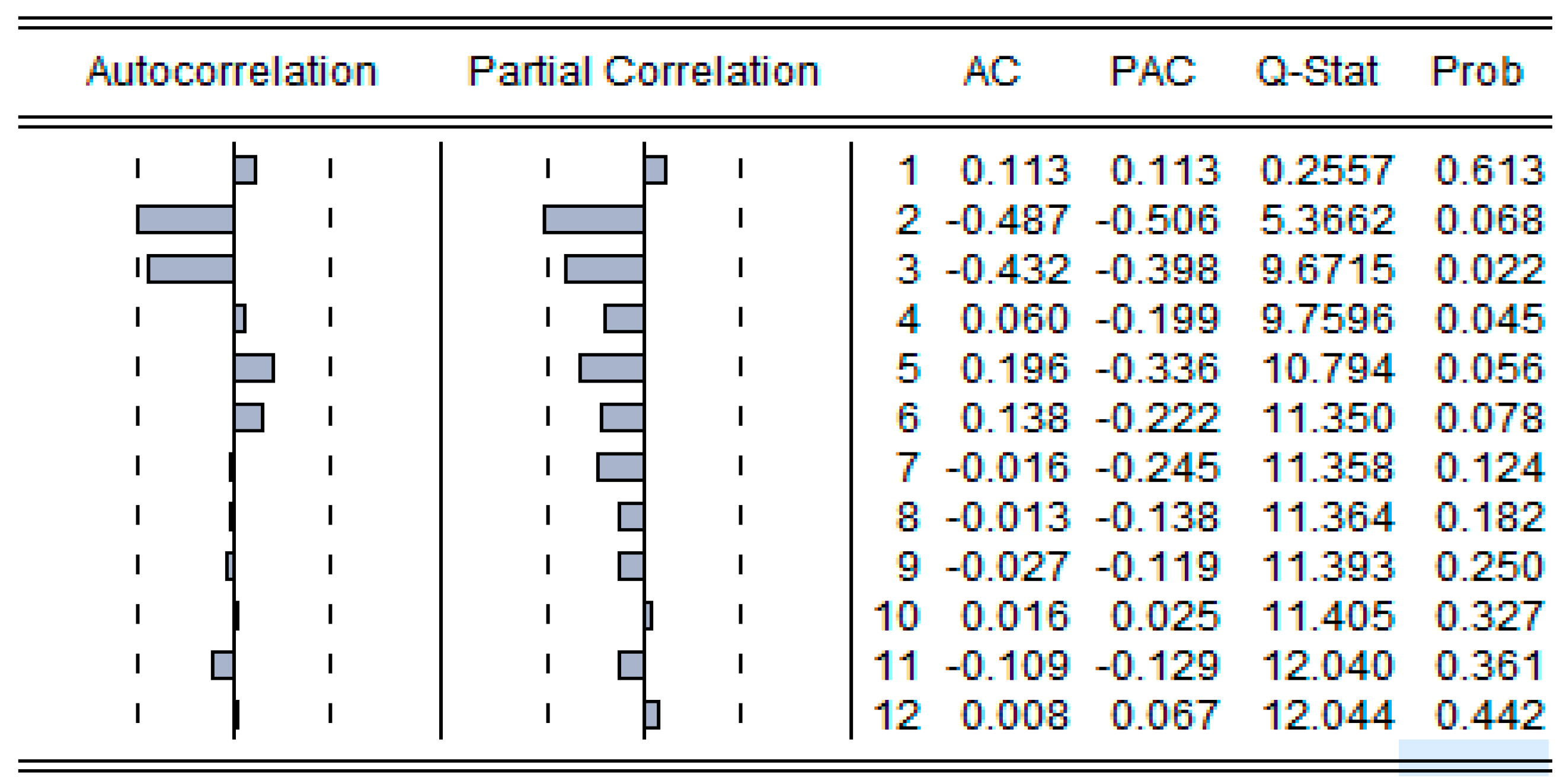
4.4. Calculation Process of the MGM-ARIMA Combined Model

The core of the combined model calculation is using ARIMA model to correct the forecasting residuals of the MGM. In the section above, the forecasting result of the MGM has already been presented. The residual sequence can be obtained via subtraction.

The first step for ARIMA model is the unit root test of residual sequence, the purpose of which is to determine the order of difference. The differential order to make the sequence stationary is represented by the value of parameter ‘d’ in ARIMA model. Appendix A

Table A2. The Result of unit root test.

Augmented Dickey-Fuller		t-Statistic	Prob. *
Test statistic		−4.13621	0.0269
Test critical values:	1% level	−4.72836
	5% level	−3.75974
	10% level	−3.32498

* Denotes rejection of the hypothesis at the 0.05 level.

shows the result after zero-order difference. The value of a T test is between 1% and 5%. Therefore, we can consider that under a 95% confidence interval, the sequence is stationary and d = 0.

After determining the solution of differential equation, we can obtain the values of ‘p’ and ‘q’ by drawing the relevant coefficient figure. Figure 4 is relevant coefficient figure of the sequence after zero-order difference. Here, the auto-correction coefficient figure can reflect the value of ‘q’ and the partial auto-correction figure present the value of ‘p’.

Knowing the value of ‘d’, we can get ‘p’ and ‘q’ from the correlation coefficient diagram. Comparing the three sets of possible values in

Table 2. Results of R value test.

ARIMA (p, 0, q)	R Value
(5, 0, 3)	0.634
(4, 0, 3)	0.549
(5, 0, 2)	0.614

, we decide to select ARIMA (5, 0, 3), because of its maximum R value.

Figure 4 shows that the partial auto-correction figure becomes stationary after five-order difference and the auto-correction coefficient figure becomes stationary after three-order difference; thus p = 5 and q = 3. Establish the ARIMA (5, 0, 3) model in SPSS software and then the corrected residuals can be obtained, as is shown in Appendix A

Table A3. Initial error and corrected error of residual sequence.

Year	Error of MGM	Error Forecast by ARIMA (5, 0, 3)
2000	0.0000	−1.21
2001	3.4894	−1.17
2002	−4.3812	−1.38
2003	−0.9070	−3.24
2004	1.9398	−2.64
2005	−9.8511	−1.97
2006	−6.3175	−1.62
2007	1.7831	5.12
2008	12.3692	10.5
2009	−2.0981	−0.69
2010	−7.4760	−6.96
2011	−7.4566	−7.17
2012	−1.9373	−0.24
2013	1.8335	1.93
2014	3.4164	0.58
2015	−5.5212	−4.18
2016	0.9243	−0.11
2017		−1.93
2018		−2.39
2019		−5.61
2020		−1.79
2021		0.91
2022		1.41
2023		−1.8
2024		−3.55
2025		−3.6
2026		−2.48
2027		−1.71
2028		−0.84
2029		−0.4
2030		−1

. Based on the corrected residual sequence and original sequence, the final forecasting value of the combined model can be acquired by calculation. Figure 5 shows that the difference between fitted value and true value is very small and the forecasting result is identical to the first two models, which all show a decreasing trend.

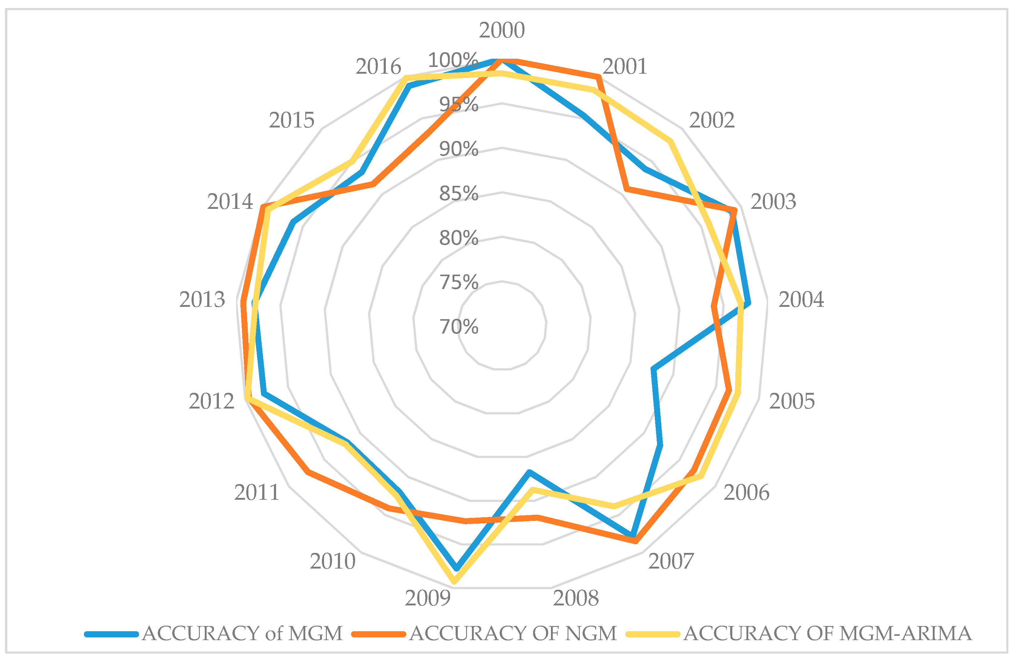
4.5. Goodness Test of Model

To judge the goodness of the three models, we use the mean absolute percent error (MAPE) to calculate their accuracy. The specific evaluation criteria for MAPE is as follows: the value of MAPE between 20–50% indicates a reasonable forecasting effect; 10–20% indicates a good forecasting effect; 0–10% indicates an excellent forecasting effect. Here, the calculation equation for the mean absolute percent error (MAPE) is as follows:

$$\mathrm{MAPE}=\frac{\left|Y_t^{*}-Y_t\right|/Y_t}{N}$$

(27)

where: $Y_t$ represents the original value; $Y_t^{*}$ represents the predicted value; N represents the number of sample data.

As is shown in

Table 3. Goodness of fit.

	MGM	NGM	MGM-ARIMA
MAPE	4.938%	3.821%	3.439%

, the MAPE of the three models all remains within 5%. Therefore, the forecasting effects are excellent. This indicates that the forecasting models used in this paper are extremely applicable and the accuracy is very high.

In addition, the relative error of each year at the fitting stage can be calculated and the method of 1-relative error can be adopted.

Figure 6 shows the accuracy of the three forecasting models. We can see that the forecasting goodness of these three models exceeds 85%, and the average accuracy is 95%, in spite of the different accuracy of each year. In a word, the reliability of these three models is very high.

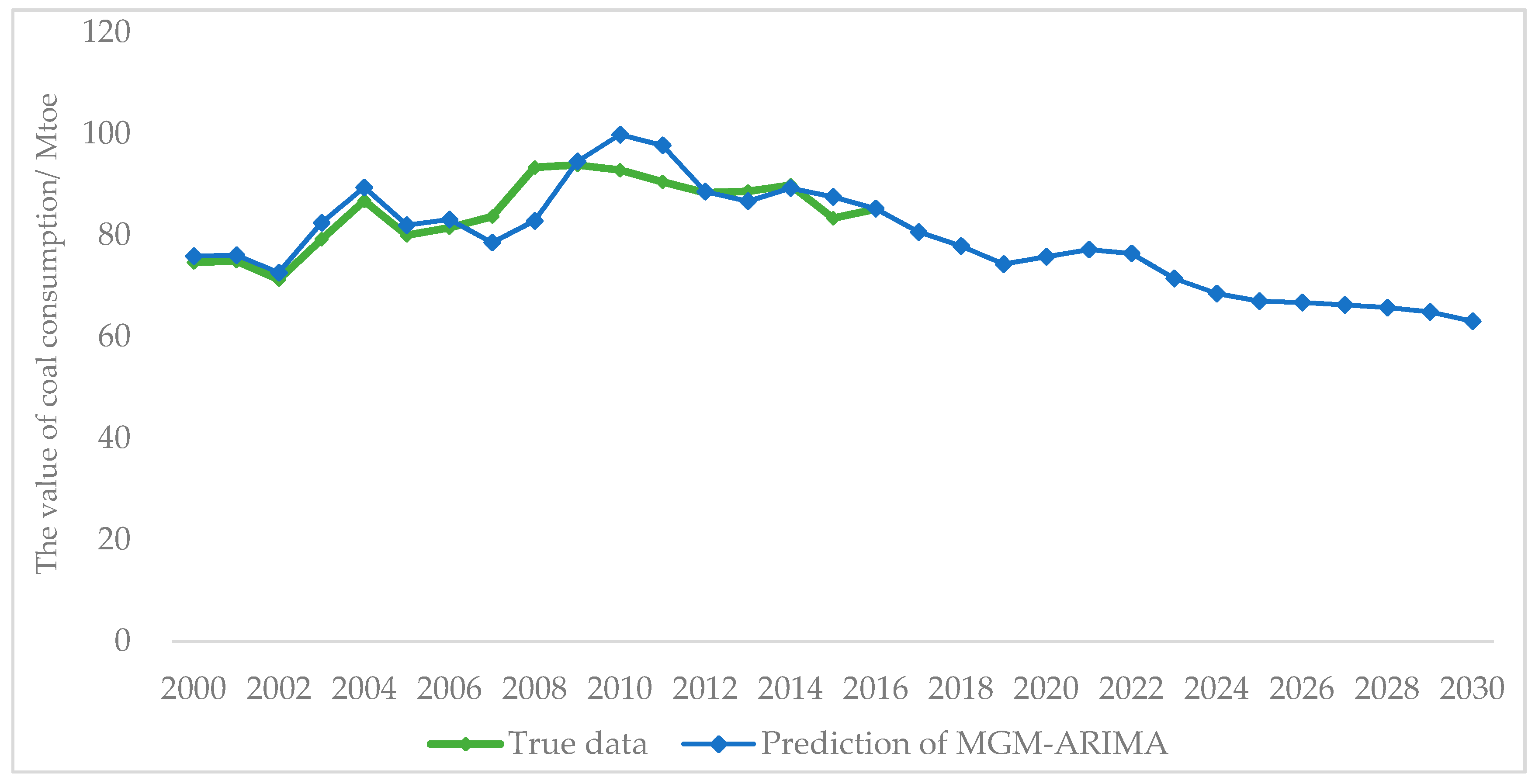
4.6. Forecast Results and Discussion

Table 4. Final forecasting period 2017–2030 (Unit: Mtoe (Million Tons of Oil Equivalent)).

Year	MGM	NGM	MGM-ARIMA
2017	82.5647	82.1295	80.6347
2018	80.2526	81.5579	77.8626
2019	79.9076	80.1653	74.2976
2020	77.5388	78.6682	75.7488
2021	76.265	77.1433	77.175
2022	74.9854	75.6323	76.3954
2023	73.2503	74.1566	71.4503
2024	72.0452	72.7238	68.4952
2025	70.6119	71.3346	67.0119
2026	69.2123	69.9882	66.7323
2027	67.9547	68.6824	66.2447
2028	66.583	67.4154	65.743
2029	65.3007	66.186	64.9007
2030	64.0417	64.9928	63.0417

presents the forecasting results of South Africa’s coal consumption in 2017–2030, and it shows that the coal consumption of South Africa will follow a stable decrease in future. This result is in line with the judgment based on the trend of South Africa’s electricity demand by 2030. Even, there are no studies related to coal consumption forecasting of South Africa. However, Inglesi et al. applied the Engle-Granger methodology for co-integration to predict long-term centricity demand in South Africa and the results showed that the South Africa’s electricity demand would reduce by 24–27% in 2030 [45]. In other words, it can indirectly indicate coal consumption may continue to decrease by 2030 because 90% of the electricity is generated from coal [46]. Besides, the decline trend of coal consumption is also consistent with the direction of policy adjustment in South African government.

For this forecasting result, we will discuss from the following aspects:

First, the mean absolute percent error of the forecasting models (MGM, NGM, MGM-ARIMA) has averaged 4 percent. On the one hand, the existing error assessment criteria clearly states that as long as the value of MAPE is less than 5%, the prediction effect of the model is excellent. The three values of MAPE given in Table 3 are all less than 5%, which implies that the forecasting results in this study are very convincing. On the other hand, these three models still have some deficiencies in prediction. For example, these models belong to the category of time series forecasting models. The time series prediction model only shows good effect at the simulation of the sequence itself. However, the future trend of a sequence is not only influenced by its historical data, but also by other variables. In other words, this prediction model used in this study cannot reflect the effect of other factors on the system. Neglecting the changes in internal factors maybe lead to inaccurate predictions, which need to be overcome in subsequent studies.

Second, coal consumption’s downward trend is related to changes in the energy structure of the world today. With the continuous decline in the running cost of natural gas, exports of natural gas continue to increase. This has led to the fact that coal has become less competitive. Apart from this, with the emphasis on air pollution and climate warming, more and more investment has been made in renewable energy power generation equipment. In other words, alternatives to coal, such as wind, solar energy, and hydropower, are becoming commonplace.

Third, the downward trend of coal consumption in the future will have an impact on South Africa’s coal development and policy formulation. For coal development, although the future coal consumption is declining, it is still the major source of power generation in a short period of time. Thus, future investment should be placed on the improvement of existing power equipment and the development of cleaning equipment. For policy formulation, the South African government should gradually reduce the dependence on coal over the next 14 years. At the same time, policy formulation should be focused on how to reduce the production costs of natural gas. In addition, the subsidies of renewable energy power generation equipment should be strengthened continuously.

5. Conclusions

South Africa is a country that the energy sources are diversified, such as solar energy and wind energy [12,47,48]; however, its coal consumption represents 88.7% of the total consumption of the whole African continent. In addition, it covers 69.6% of the energy consumption of South Africa. The significant coal consumption leads to a large amount of carbon emission in South Africa. Furthermore, it will cause global ecological deterioration. Therefore, the longterm prediction of South Africa’s coal consumption can provide a data support for global environmental governance.

This study adopted linear (MGM and MGM-ARIMA) and nonlinear (NGM) models to forecast South Africa’s coal consumption in 2017–2030. The error in these three forecasting models is all below 5%: MGM (4.9%), NGM (3.8%), and MGM-ARIMA (3.4%). The small forecasting error indicates the high reliability of the three models in forecasting the long-term coal consumption. During the next 14 years, the development tendency of South Africa’s coal consumption will follow an annual decrease of 1.9%. This result shows that South Africa is reducing its dependence on coal. This also indicates that the strategy of increasing the use of renewable energy, formulated by the South African government, has scored remarkable achievements, which contributes to the carbon emission reduction [49,50].

References

1. Ouyang, X.; Lin, B. An analysis of the driving forces of energy-related carbon dioxide emissions in China’s industrial sector. Renew. Sustain. Energy Rev. 2015, 45, 838–849. [Google Scholar] [CrossRef]
2. Mcglade, C.; Ekins, P. The geographical distribution of fossil fuels unused when limiting global warming to 2 °C. Nature 2015, 517, 187–190. [Google Scholar] [CrossRef] [PubMed] [Green Version]
3. Höök, M.; Tang, X. Depletion of fossil fuels and anthropogenic climate change—A review. Energy Policy 2013, 52, 797–809. [Google Scholar] [CrossRef] [Green Version]
4. Marland, G.; Boden, T.A.; Andres, R.J.; Brenkert, A.L.; Johnston, C. Global, Regional, and National Fossil-Fuel CO2 Emissions; Carbon Dioxide Information Analysis Center (CDIAC): Oak Ridge, TN, USA, 2012.
5. Wang, Q.; Zhao, M.; Li, R.; Su, M. Decomposition and decoupling analysis of carbon emissions from economic growth: A comparative study of China and the United States. J. Clean. Product. 2018, 197, 178–184. [Google Scholar] [CrossRef]
6. Peters, G.P.; Marland, G.; Hertwich, E.G.; Saikku, L.; Rautiainen, A.; Kauppi, P.E. Trade, transport, and sinks extend the carbon dioxide responsibility of countries: An editorial essay. Clim. Chang. 2009, 97, 379–388. [Google Scholar] [CrossRef]
7. Wang, Q.; Chen, X. Energy policies for managing China’s carbon emission. Renew. Sustain. Energy Rev. 2015, 50, 470–479. [Google Scholar] [CrossRef]
8. Zhang, Y.J.; Da, Y.B. The decomposition of energy-related carbon emission and its decoupling with economic growth in China. Renew. Sustain. Energy Rev. 2015, 41, 1255–1266. [Google Scholar] [CrossRef]
9. World Bank. The Wor ld Bank Data; World Bank: Washington, DC, USA, 2007; Available online: http://data.worldbank.org (accessed on 14 July 2018).
10. British Petroleum. Statistical Review of World Energy; British Petroleum: London, UK, 2017; Available online: https://www.bp.com/zh_cn/china/reports-and-publications/_bp_2017-_.html (accessed on 14 July 2018).
11. McEwan, C. Spatial processes and politics of renewable energy transition: Land, zones and frictions in South Africa. Political Geogr. 2017, 56, 1–12. [Google Scholar] [CrossRef]
12. Aliyu, A.K.; Modu, B.; Tan, C.W. A review of renewable energy development in Africa: A focus in South Africa, Egypt and Nigeria. Renew. Sustain. Energy Rev. 2018, 81, 2502–2518. [Google Scholar] [CrossRef]
13. Pollet, B.G.; Staffell, I.; Adamson, K.A. Current energy landscape in the Republic of SouthAfrica. Int. J. Hydrogen Energy 2015, 40, 16685–16701. [Google Scholar] [CrossRef]
14. Wang, Q.; Li, R. Journey to burning half of global coal: Trajectory and drivers of China’s coal use. Renew. Sustain. Energy Rev. 2016, 58, 341–346. [Google Scholar] [CrossRef]
15. Apergis, N.; Loomis, D.; Payne, J.E. Are fluctuations in coal consumption transitory or permanent? Evidence from a panel of US states. Appl. Energy 2010, 87, 2424–2426. [Google Scholar] [CrossRef]
16. Gurgul, H.; Lach, Ł. The role of coal consumption in the economic growth of the Polish economy in transition. Energy Policy 2011, 39, 2088–2099. [Google Scholar] [CrossRef] [Green Version]
17. Kumar, U.; Jain, V.K. Time series models (Grey-Markov, Grey Model with rolling mechanism and singular spectrum analysis) to forecast energy consumption in India. Energy 2010, 35, 1709–1716. [Google Scholar] [CrossRef]
18. Yoo, S.H. Causal relationship between coal consumption and economic growth in Korea. Appl. Energy 2006, 83, 1181–1189. [Google Scholar] [CrossRef]
19. Bildirici, M.E.; Bakirtas, T. The relationship among oil, natural gas and coal consumption and economic growth in BRICTS (Brazil, Russian, India, China, Turkey andSouth Africa) countries. Energy 2014, 65, 134–144. [Google Scholar] [CrossRef]
20. Wang, Q.; Li, R. Decline in China’s coal consumption: An evidence of peak coal or a temporary blip? Energy Policy 2017, 108, 696–701. [Google Scholar] [CrossRef]
21. Wang, Q.; Jiang, X.-T.; Li, R. Comparative decoupling analysis of energy-related carbon emission from electric output of electricity sector in Shandong Province, China. Energy 2017, 127, 78–88. [Google Scholar] [CrossRef]
22. Ziramba, E. Disaggregate energy consumption and industrial production in South Africa. Energy Policy 2009, 37, 2214–2220. [Google Scholar] [CrossRef]
23. Shahbaz, M.; Tiwari, A.K.; Nasir, M. The effects of financial development, economic growth, coal consumption and trade openness on CO2 emissions in South Africa. Energy Policy 2013, 61, 1452–1459. [Google Scholar] [CrossRef] [Green Version]
24. Odhiambo, N.M. Coal Consumption and Economic Growth in South Africa: An Empirical Investigation; Academic Forum: Santa Rosa, CA, USA, 2016; p. 15. [Google Scholar]
25. Menyah, K.; Wolde-Rufael, Y. Energy consumption, pollutant emissions and economic growth in South Africa. Energy Econ. 2010, 32, 1374–1382. [Google Scholar] [CrossRef]
26. Al-Mulali, U.; Che, N.B.C.S. The impact of energy consumption and CO2 emission on the economic and financial development in 19 selected countries. Renew. Sustain. Energy Rev. 2012, 16, 4365–4369. [Google Scholar] [CrossRef]
27. Alton, T.; Arndt, C.; Davies, R.; Hartley, F.; Makrelov, K.; Thurlow, J.; Ubogu, D. Introducing carbon taxes in South Africa. Appl. Energy 2014, 116, 344–354. [Google Scholar] [CrossRef]
28. Ediger, V.Ş.; Akar, S. ARIMA forecasting of primary energy demand by fuel in Turkey. Energy Policy 2007, 35, 1701–1708. [Google Scholar] [CrossRef]
29. Org, Z. Day-ahead wind speed forecasting using f-ARIMA models. Renew. Energy 2009, 34, 1388–1393. [Google Scholar]
30. Farahbakhsh, H.; Ugursal, V.I.; Fung, A.S. A residential end-use energy consumption model for Canada. Int. J. Energy Res. 2015, 22, 1133–1143. [Google Scholar] [CrossRef]
31. Choi, J.; Roberts, D.C.; Lee, E.S. Forecasting Oil Production in North Dakota Using the Seasonal Autoregressive Integrated Moving Average (S-ARIMA). Nat. Resour. 2015, 6, 16–26. [Google Scholar] [CrossRef]
32. Berwick, M.; Malchose, D. Forecasting North Dakota Fuel Tax Revenue and License and Registration Fee Revenue; Upper Great Plains Transportation Institute: Fargo, ND, USA, 2012. [Google Scholar]
33. Dejuán, Ó.; López, L.A.; Tobarra, M.Á.; Zafrilla, J. A Post-Keynesian Age Model to Forecast Energy Demand in Spain. Econ. Syst. Res. 2013, 25, 321–340. [Google Scholar] [CrossRef]
34. Lochin, E.; Fladenmuller, A.; Moulin, J.Y.; Fdida, S. Energy Consumption Models for Ad-Hoc Mobile Terminals; Med-Hoc Net: Paries, France, 2003. [Google Scholar]
35. Okumus, I.; Dinler, A. Current status of wind energy forecasting and a hybrid method for hourly predictions. Energy Convers. Manag. 2016, 123, 362–371. [Google Scholar] [CrossRef]
36. Yu, F.; Xu, X. A short-term load forecasting model of natural gas based on optimized genetic algorithm and improved BP neural network. Appl. Energy 2014, 134, 102–113. [Google Scholar] [CrossRef]
37. Plessis, W.D. Energy efficiency and the law: A multidisciplinary approach. S. Afr. J. Sci. 2015, 111, 1–8. [Google Scholar] [CrossRef] [Green Version]
38. Shaikh, F.; Ji, Q.; Shaikh, P.H.; Mirjat, N.H.; Uqaili, M.A. Forecasting China’s natural gas demand based on optimised nonlinear grey models. Energy 2017, 140, 941–951. [Google Scholar] [CrossRef]
39. Lee, Y.S.; Tong, L.I. Forecasting energy consumption using a grey model improved by incorporating genetic programming. Energy Convers. Manag. 2011, 52, 147–152. [Google Scholar] [CrossRef]
40. Li, S.; Yang, X.; Li, R. Forecasting China’s Coal Power Installed Capacity: A Comparison of MGM, ARIMA, GM-ARIMA, and NMGM Models. Sustainability 2018, 10, 506. [Google Scholar] [CrossRef]
41. Chen, L.; Lin, W.; Li, J.; Tian, B.; Pan, H. Prediction of lithium-ion battery capacity with metabolic grey model. Energy 2016, 106, 662–672. [Google Scholar] [CrossRef]
42. Box, G.E.P.; Jenkins, G. Time Series Analysis, Forecasting and Control; Holden-Day, Incorporated: San Francisco, CA, USA, 1990; pp. 238–242. [Google Scholar]
43. Wang, Q.; Li, S.; Li, R.; Ma, M. Forecasting U.S. Shale Gas Monthly Production Using a Hybrid ARIMA and Metabolic Nonlinear Grey Model. Energy 2018, 160, 378–387. [Google Scholar] [CrossRef]
44. British Petroleum. Statistical Review of World Energy; British Petroleum: London, UK, 1965–2017; Available online: https://www.bp.com/en/global/corporate/energy-economics/statistical-review-of-world-energy/downloads.html (accessed on 14 July 2018).
45. Inglesi, R. Aggregate electricity demand in South Africa: Conditional forecasts to 2030. Appl. Energy 2010, 87, 197–204. [Google Scholar] [CrossRef] [Green Version]
46. Thopil, G.A.; Pouris, A. Water usage forecasting in coal based electricity generation: The case of South Africa. Energy Procedia 2015, 75, 2813–2818. [Google Scholar] [CrossRef]
47. Othieno, H.; Awange, J. Energy Resources in Africa; Springer International Publishing: Basel, Switzerland, 2016. [Google Scholar]
48. Wang, Q.; Li, R. Natural gas from shale formation: A research profile. Renew. Sustain. Energy Rev. 2016, 57, 1–6. [Google Scholar] [CrossRef]
49. Azimoh, C.L.; Klintenberg, P.; Wallin, F.; Karlsson, B.; Mbohwa, C. Electricity for development: Mini-grid solution for rural electrification in South Africa. Energy Convers. Manag. 2016, 110, 268–277. [Google Scholar] [CrossRef] [Green Version]
50. Eberhard, A.; Kåberger, T. Renewable energy auctions in South Africa outshine feed-in tariffs. Energy Sci. Eng. 2016, 4, 190–193. [Google Scholar] [CrossRef] [Green Version]
Figure 1. Value of MGM model parameters. Note: The values of ‘a’ and ‘b’ in Figure 1 correspond to Equation (13). Figure 1 shows the solution of ‘a’ and ‘b’ in Equation (13).
Sustainability 10 02552 g001
Figure 2. The forecasting of the MGM model.
Sustainability 10 02552 g002
Figure 3. Forecasting of the NGM model.
Sustainability 10 02552 g003
Figure 4. Correlation plot of the stationary sequence.
Sustainability 10 02552 g004
Figure 5. Forecasting of the MGM-ARIMA model.
Sustainability 10 02552 g005
Figure 6. Accuracy of forecasting of all three models.
Sustainability 10 02552 g006