Article

A Rice Mapping Method Based on Time-Series Landsat Data for the Extraction of Growth Period Characteristics

1
College of Natural Resources and Environment, South China Agricultural University, Guangzhou 510642, China
2
Key Laboratory of the Ministry of Land and Resources for Construction Land Transformation, South China Agricultural University, Guangzhou 510642, China
3
Guangdong Provincial Key Laboratory of Land Use and Consolidation, South China Agricultural University, Guangzhou 510642, China
4
Guangdong Province Land Information Engineering Technology Research Center, South China Agricultural University, Guangzhou 510642, China
5
College of Agriculture and Animal Husbandry, Qinghai University, Xining 810016, China
6
Guizhou Academy of Sciences, Guiyang 550001, China
7
ASRC Federal, U.S. Geological Survey Earth Resources Observation and Science (EROS), Sioux Falls, SD 57198, USA
8
Department of Geography and Environmental Resources, College of Liberal Arts, Southern Illinois University Carbondale (SIUC), Carbondale, IL 62901, USA
*
Authors to whom correspondence should be addressed.
Sustainability 2018, 10(7), 2570; https://doi.org/10.3390/su10072570
Submission received: 4 July 2018 / Revised: 18 July 2018 / Accepted: 19 July 2018 / Published: 23 July 2018
(This article belongs to the Section Sustainable Agriculture)

Abstract

:
The rapid and accurate acquisition of rice cultivation information is very important for the management and assessment of rice agriculture and for research on food security, the use of agricultural water resources, and greenhouse gas emissions. Rice mapping methods based on phenology have been widely used but further studies are needed to clearly quantify the rice characteristics during the growth cycle. This paper selected the area where rice agriculture has undergone tremendous changes as the observation object. The rice areas were mapped in three time periods during the period from 1993 to 2016 by combining the characteristics of the harvested areas, flooded areas, and the time interval when harvesting and flooding occurred. An error matrix was used to determine the mapping accuracy. After exclusion of clouds and cloud shadows, the overall accuracy of the paddy fields was higher than 90% (90.5% and 93.5% in period 1 and period 3, respectively). Mixed pixels, image quality, and image acquisition time are important factors affecting the accuracy of rice mapping. The rapid economic development led to an adjustment of people’s diets and presumably this is the main reason why rice cultivation is no longer the main agricultural production activity in the study area.

1. Introduction

Rice agriculture plays an important role in global food security assessment [1], utilization of agricultural water resources [2], greenhouse gas emissions [3], bird flu epidemic prevention [4] and other research. Rice cultivation areas are vulnerable to climate change, agricultural policy adjustments, land-use changes, and other factors. For example, due to rapid population growth and urbanization, China’s rice acreage has generally declined between 2005 and 2015 [5]. Due to the warming of the climate and increasing demand for food, in the past ten years, the area of rice cultivation has rapidly expanded in high latitudes, such as Northeast Asia [6]. Information on the spatial variation of these rice cultivation areas is crucial for related research on rice agriculture.
Rice mapping using remote sensing methods is an important approach for monitoring rice production. New mapping methods are still being proposed and include methods such as the image statistics methods based on reflectivity and vegetation indices [7,8,9] and time-series analysis methods based on vegetation indices and radar echoes [10,11,12]. Currently, rice mapping methods based on key phenological phases are the most widely used and stable rice mapping methods. Due to the phenological differences of the rice plants in different growth periods, such as the transplanting period [13] and the tillering period [14], significant differences exist between rice and non-rice land-use types. For example, since a mixed signal exists for rice seedlings and the flooded areas in the initial growth stage, the signal is extracted from the vegetation- or water-sensitive spectral bands or remote sensing indices [6,15,16,17,18].
Phenology-based rice mapping methods require a quantified expression. Crop phenology refers to the study of periodic crop life cycles and the changes that occur over time. It is quite intuitive and simple to capture the changes in a crop’s growth cycle. The method of relying on a single scene to capture the characteristics of the phenological period is influenced by the surrounding surface conditions. In order to eliminate the interference of other surface conditions in single-view images, the creation of non-paddy field masks (forests, wetlands, grasslands, etc.) is a prerequisite for rice mapping [6,17,19]. This undoubtedly increases the steps used in rice mapping and it is difficult to assess the error associated with this step. Therefore, studies have been conducted to map rice in a complex landscape where rice and wetlands coexist [20,21].
Land use changes and rapid economic development are considered important factors affecting global rice production. The Pearl River Delta is one of the fastest-growing regions in the global economy and this has been especially noticeable over the past 30 years. Rapid economic development and increased urbanization have greatly changed the original land use conditions in this region [22,23]. Air pollution [24,25], water resources security [26,27], soil pollution [28,29], human activities [30], and other issues that resulted from this process have also attracted attention. In this study, we selected traditional rice agricultural areas in the Pearl River Delta. By capturing the changes in the rice planting areas, we determine and discuss the impacts and challenges that these changes have on rice mapping.
With the increased availability of high-quality time-series remote sensing images, it is possible to use time-series data to capture the characteristics of the entire growth period of rice in paddy fields. Therefore, in this study, we propose to use an intuitive classifier to extract the phenophase characteristics of rice from time-series data to distinguish rice fields from non-rice land types, thereby reducing errors and uncertainties for creating non-rice masks. Specifically, the main objectives of this study are (1) to explore the ability of Landsat images to reflect changes in the phenophase characteristics of rice at different growth stages; (2) to examine the accuracy of the rice mapping results in the study area for different time periods; (3) to analyze the application potential of this research method based on three factors: image quality, image acquisition time, and mixed pixels; (4) to determine and discuss the changes in the traditional rice agriculture in the study area.

2. Study Area

The study area is Zengcheng City in the central part of Guangdong Province and in the east of Guangzhou City, located in the northeast corner of the Pearl River Delta (Figure 1). The geographical coordinates of the study area are 23°05′–23°37′ N and 113°32′–114°00′ E. The research area is located in the southern subtropical zone and has a maritime monsoon climate with hot and rainy conditions. There is no winter season and because of the long growing season, the area can be cultivated throughout the year. The elevation decreases from north to south and the land is roughly divided into middle-low mountains/valleys, hilly land, and alluvial plains. Each land type covers about one-third of the total area (Figure 1c). Most of the cultivated land in the area is located in the hills and alluvial plains. The soil is rich in organic matter and suitable for planting crops.
The study area covers about 1741 sq km. In 2015, the registered population of the area was 872,500 and was comprised of the non-agricultural population of 231,000 and the agricultural population of 641,500 (Table 1). The area is located in the traditional double-season rice planting area in South China and has a high-quality rice variety with local characteristics. This region is located in an important part of the Pearl River Delta connecting Macau to Hong Kong. Since the end of the last century, Zengcheng has gradually transformed itself into an emerging industrial city. Its annual gross agricultural output value as a percentage of the gross domestic product (GDP) fell from 13% in 1995 to 5% in 2015.

3. Materials and Methods

3.1. Data and Preprocessing

3.1.1. Data

In 2016, field surveys were conducted on the rice cultivation in the study area and data on the rice planting history and cropping systems in the region were collected, as well as land use maps for the region in 2005 and 2015. Remote sensing images over three time periods were collected (Table 2). Landsat Thematic Mapper (TM) images were obtained for the first two time periods and Landsat 8 Operational Land Imager (OLI) images were used for the third time period. The TM and OLI data used in this study were sourced from https://glovis.usgs.gov and were the L1TP Landsat surface reflectance data product. These data were used to ensure the reliability and consistency of the data source.

3.1.2. Data Preprocessing

1. Top of Atmosphere (TOA) Reflectance Correction
We use a TOA reflectance correction method that uses only the Earth–Sun geometry to define the reflectivity of the satellite measurements and an atmospheric correction was not applied. We compare the time-series images of the Landsat products in three time periods instead of analyzing the images separately [31]. TOA image correction has been able to meet the time series of remote sensing index analysis, rather than the absolute value of these indices. Because the surface changes of the rice fields (water-vegetation-soil) in the time series are far greater than any variability caused by atmospheric influences, an atmospheric correction was not required [17].
2. TM image cloud and cloud shadow mask
For the TM images, cloud masks were created using the Automatic Cloud Cover Assessment (ACCA) [32] and the Function of mask (Fmask) methods [33]. The ACCA method extracts the thick cloud boundary accurately and the Fmask method is more suitable for thin clouds (Figure 2). However, neither of these methods is ideal for cloud shadows.
The position of the cloud shadows is affected by factors such as the sun angle, the angle of the satellite sensors, the height of the clouds, and the terrain relief. In a single image, the height of the clouds is not uniform and, therefore, the cloud shadows have different degrees of offset with respect to the position of the clouds but the offset of the shadows generated by the same type of cloud in the same scene is nearly similar. Therefore, we visually interpret the type of clouds in a single scene and move the cloud mask to obtain a corresponding cloud shadow mask (Figure 2c–f).
3. OLI image cloud and cloud shadow mask
For the OLI image, we select the pixels in the Quality Assessment Band marked as “not affected by instruments or clouds” as a mask to remove the cloud and cloud shadows in the scene.

3.2. Vegetation Index and Water Body Index

In this study, the characteristics of the key phenological changes of the rice were captured using the normalized difference vegetation index (NDVI) [34] and the modified normalized difference water index (MNDWI) [35]. The NDVI is one of the most widely used remote sensing spectral indices for monitoring vegetation density and health. The NDVI values range from −1 to 1. The index is easy to interpret and compare, and compensates for the differences between images as a result of different atmospheric conditions and satellite instrument characteristics. Its calculation formula is
  NDVI = ρ NIR ρ RED ρ NIR + ρ RED  
where ρ NIR is the near-infrared band (0.76–0.90   μ m ) and ρ RED is the red band (0.63–0.69   μ m ). We use the NDVI as an indicator of crop harvesting characteristics, taking into account that the NDVI is prone to saturation in high vegetation cover but sensitive to low vegetation cover changes. There is no winter in the study area and the vegetation remains green throughout the year. During the crop harvesting season, the NDVI loses its ability to detect change due to the saturation of high vegetation areas; this can result in misinterpretations of the characteristics of the harvested crops and the changes in vegetation coverage of non-harvested crop lands.
The MNDWI is an improvement over the normalized difference water index (NDWI) and has been shown to be more applicable to the detection of open waters while suppressing the background noise of vegetation, soil, and developed land [35,36]. The formula is
  MNDWI = ρ GREEN ρ SWIR ρ GREEN + ρ SWIR  
where ρ GREEN is the green band (0.52–0.60   μ m ) and ρ SWIR is the mid-infrared band (1.60–1.70   μ m ). The green band is sensitive to differences in water turbidity, sediments, and pollution and the mid-infrared band shows strong contrast between the land and water features due to high water absorption and strong reflection of vegetation and natural landscapes [37]. Therefore, the MNDWI is more suitable for extracting the water bodies located in built-up areas because, unlike the NDWI, it reduces or even eliminates land noise [35].

3.3. Rice Mapping Method

The rice mapping consisted of three steps, including extraction of the harvested areas, the flooded areas, and the time interval when harvesting and flooding occurred. The process is as follows (Figure 3):
(1) Extraction of the harvested areas: The high-vegetation coverage area mask from June to October (NDVI > 0.6/0.5) and the low-vegetation coverage area mask from July to November (0 < NDVI < 0.4/0.3) are used. An area is classified as harvested when a high-vegetation area changes to a low-vegetation area over one month. The time of the harvest is the image time of the low vegetation mask (Figure 3c–e). (2) Extraction of the flooded areas: the water area mask from March to August (MNDWI > 0/0.1) and the non-water area mask from April to September (MNDWI < 0) are used. An area is classified as flooded when a non-water area changes into a water area over one month. The time of the flooding is the image time of the water area mask (Figure 3f–h). (3) An area is classified as a paddy field when the overlapping area of the harvested areas and the flooded areas is separated by about 100 days (Figure 3i).

3.4. Accuracy Assessment

Stratified random sampling was used to obtain the test samples for the rice classification. At the pixel scale (regardless of the problem of mixed pixels), the land types include rice fields, non-paddy fields and, within the rice field class, small rice fields (10 Landsat pixels and below), medium-sized rice fields (11 to 50 Landsat pixels), and large rice fields (51 Landsat pixels and above). In order to classify the size of the fields, in the Landsat original image, the agricultural land area (land use status map) was classified using object-oriented segmentation and the field types are determined based on the number of pixels.
The 2016 test samples were obtained using field measurements and the test samples of the remaining years were extracted from the original Landsat image and the corresponding scene in Google EarthTM [17]. In order to determine the mapping accuracy, an error matrix (at the pixel scale) is used to evaluate the user’s accuracy, the producer’s accuracy, and the overall accuracy. The sampling design used to obtain the test samples affects the mapping accuracy and the variance of the estimated parameters is used to explain the uncertainty of the sampling design, that is, the estimated variances of the overall accuracy, the user’s accuracy, and the producer’s accuracy [38]. The error matrix formulas are defined as follows:
  O = j = 1 q p jj  
where O is the overall accuracy, q is the number of classes,   i is the map class, j is the reference class, and p jj is the proportion of the area in i and j .
  U i = p ii p i ·  
where U i is the user’s accuracy of i , i is the map class, p ii is the proportion of the area of i in the map class and the reference class, and p i · is the area proportion of i in the map class.
  P   j = p jj p · j  
where P   j is the producer’s accuracy of j , and p · j is the proportion of the area of j in the reference class.
We denote the sample estimate of p ij as p ^ ij , then
  p ^ ij = W i n ij n i ·  
where W i is the area proportion of i in the map class. n ij is the number of samples whose map class is i and the test sample is j . n i · is the number of samples of i in the map class.
The standard deviation is used to quantify the sampling variability associated with the accuracy estimate. The estimated variance of the overall accuracy is
V ^ ( O ^ ) = i = 1 q W i 2 U ^ i ( 1 U ^ i ) / ( n i · 1 )  
The estimated variance of the user’s accuracy of i in the mapping result is
V ^ ( U ^ i ) = U ^ i ( 1 U ^ i ) / ( n i · 1 )  
The estimated variance of the producer’s accuracy for j in the test sample is
V ^ ( p ^   j ) = 1 N ^ · j 2 [ N j · 2 ( 1 P ^   j ) 2 U ^ j ( 1 U ^ j ) n j · 1 + p ^   j 2 i j q N i · 2 n ij n i ·   ( 1 n ij n i · ) / ( n i · 1 ) ]  
where N j is the total number of margins of j in the map class and n j is the total number of j in the test sample. N ^ · j is the total number of estimated margins for the pixels of the j in the test sample; the formula is
  N ^ · j = i = 1 q N i · n i · n ij  

4. Result

4.1. Spatio-Temporal Changes In Rice Cultivation in the Study Area

In period 1, rice cultivation was the region’s main agricultural production activity but after 20 years, the rice planting area decreased by more than 80% (Figure 4). The largest decrease in the rice planting area occurred in the southern alluvial plain. In period 1, the plain was still one of the main rice producing areas. From period 1 to period 2, the area of paddy fields decreased considerably only in the northern part of the plain; in period 3, there was only a sporadic distribution of paddy fields throughout the plains. The central hilly region, “one step behind”, experienced similar changes. From period 1 to period 2, the rice planting area shrank but it still retained the majority of the area. In period 3, the rice fields were scattered in the hilly region. Correspondingly, the northern valley has retained more rice agriculture.
Figure 5 shows that a large number of the large paddy fields (over 4.5 ha) were distributed in the study area in period 1. By the second period, large-scale rice fields were scattered only in the north of the plain and were concentrated in the central hilly region and the northern valley region. By the third period, large-scale rice fields were scattered only in the northern valleys. From period 1 to period 2, the distribution of small-scale paddy fields (less than 0.9 ha) and medium-sized rice fields (ranging from 0.9 ha to 4.5 ha) increased in the central hilly region and in the northern mountainous region. This is due to the fact that with the gradual reduction in the area of paddy fields, more and smaller areas of paddy fields occur but the overall trend indicates that the area of medium-sized rice fields and small rice fields has decreased significantly.

4.2. Mapping Accuracy

The accuracy results of the rice mapping are shown in Table 3 and Table 4. The overall accuracy of rice mapping in the three periods was 93.5%, 81.0%, and 90.5%, respectively. In the second period, the mapping results were poor (user’s accuracy and overall accuracy for rice and non-rice lands were around 80%) because cloud and cloud shadow could not be eliminated entirely in the image (see the Landsat data).
For the first and third period, the accuracy was higher for the non-rice class than the rice class (95.0% vs. 92.0%, 93.0% vs. 88.0%, respectively). The high accuracy of the non-rice class indicates that the rice class cannot be easily defined by the extraction rules defined for the harvested areas, flooded areas, and the time interval. This also explains that the user’s accuracy is higher for the rice class than the non-rice class (in periods 1 and 2 respectively, 94.8% vs. 92.2%, and 92.6% vs. 88.6%).

4.3. Influence of Rice Field Area on Mapping Accuracy

In each of the three periods, the smaller the area of a single paddy field, the lower the overall accuracy of the classification results (in period 1, 79.3% of all paddy fields were small-scale paddy fields, 88.5% were medium-sized paddy fields, and 96.0% were large-scale rice fields; in period 2, the proportions were 60.0%, 78.0%, and 86.0%, respectively; in period 3, the proportions were 76.3%, 82.0%, and 93.5%, respectively). Due to the failure of completely eliminating the cloud and cloud shadows, the mapping accuracy was generally low in period 2. After removing the cloud and cloud shadows, the mapping method used in this study is very stable with regard to the mapping accuracy of the medium-sized and large-scale rice fields (overall accuracy in periods 1 and 3 was about 90%).
The smaller the area of the paddy fields and the greater the amount of mixed pixels, the more difficult it is to determine a threshold for the remote sensing index. The area of small paddy fields is generally underestimated (the producer’s accuracies of rice mapping in the three periods were 75.3%, 64.7%, and 77.3%, respectively). Mixed pixels are common in 30-m spatial resolution images and the segmented areas of the Landsat pixels corresponding to small rice fields have a very high probability of mixed pixels. Other areas in the study area, especially other crops planted very close to the paddy fields, had almost no water present during the rice transplanting period. When the pixels of rice and non-rice crops are mixed, the MNDWI at the transplanting stage is close to or even larger than 0, resulting in a failure of extraction during masking of the flooded features, thereby reducing the mapping accuracy of the small paddy fields.

4.4. Estimated Variance of Mapping Accuracy

The overall precision, user’s accuracy, and cartographic accuracy of the rice mapping method were estimated based on the areas (number of pixels) of rice and non-rice in the classified image. By comparing and analyzing the overall precision of rice mapping in the three periods, we can observe the influence of the rice field changes in the study area on the mapping accuracy. The overall accuracy of rice mapping was highest (0.918) in period 1. During period 3, the paddy area was significantly smaller and the overall accuracy was lower (0.896). Due to the reduction of the paddy area and the influence of cloud and cloud shadows, the overall precision of the rice mapping was lowest during period 2 (0.844).
The changes in the paddy field area have a significant effect on the precision of the rice mapping. The small-scale rice fields have lower overall accuracy estimates in all periods (0.718 in period 1, 0.636 in period 2, and 0.782 in period 3). With the shrinking and disappearance of the large and medium-sized rice fields, the proportion of small rice fields increased. The overall accuracy of the small paddy fields was higher during period 3 than during period 1.
The estimated accuracy of the rice field mapping was 0.920 in period 1 and 0.720 in period 3 and the significant reduction in the estimated accuracy of the mapping showed that the paddy field area was underestimated due to the smaller size of the rice paddy area. Most of the rice fields that were underestimated were small rice fields. The accuracy of the small paddy field mapping was estimated to be 0.763 during period 1 and the values for periods 2 and 3 were 0.702 and 0.591, respectively.

4.5. Comparison of Cartographic Results with Census Data

In order to further verify the rice mapping method proposed in this study, we use socio-economic statistical data for the study area to verify the accuracy of the mapping results. The rice agriculture data in the study area is based on one year and two seasons and the difference in the planting area of the early rice and late rice is very small in the statistical data of the same period. The statistical data in Table 5 shows the average of the sown area of the early rice and late rice in the same year. In period 1, the differences between the rice mapping results and statistical data were small, 19,542 ha compared with 22,849 ha. Consistent with the results reported in Table 6, the image quality affected the extraction accuracy of the paddy fields in period 2 and the area of paddy fields during this period was seriously underestimated, especially in the hilly and valley areas where rice fields were widely distributed.

5. Discussion

5.1. Advantages of this Study’s Rice Mapping Method

The farming system in the study area is 1 year 2 ripe. The suitable rice planting time ranges from March to November each year and the rice growth period lasts about 120 days and is divided into four main growth stages [39]. The classification method proposed in this study is based on the unique cyclic characteristics of paddy fields that include the periods of submergence, vegetation cover, and a mixed surface of bare soil/vegetation residue. Among them, the change from the vegetation cover period to the bare soil/vegetation residue period represents the harvesting characteristics of crops. Surfaces that feature this characteristic include crops such as rice (the marine monsoon climate in the study area limits the sudden drop in vegetation index caused by fallen leaves and other vegetation types). Approximately 100 days prior to the harvest period, the flooding of the fields represents the water–vegetation surface change that distinguishes rice fields from other crops. The combination of using the harvested areas, flooded areas, and the time interval between flooding and harvesting (about 100 days) separates most rice fields from non-rice fields in the study area, including riverbanks and wetlands because these sites do not exhibit the harvesting characteristics. These surface change characteristics are common in low-latitude tropical regions; therefore, the method can be used in other areas at low latitudes. However, for high latitudes, the applicability of this method requires further testing due to factors such as defoliation in non-rice regions that may interfere with the extraction of harvested areas.

5.2. Challenges of the Rice Mapping Method

5.2.1. Mixed Pixels

As rice fields are becoming more fragmented, the mixed pixel problem inherent in 30-m Landsat images will inevitably increase and this strongly affects the classification accuracy. However, this effect merely places higher requirements on the spatial resolution of the image data and does not change the quantitative differences between rice and non-rice land types. With the increasing availability of high-resolution remote sensing data and new data fusion methods resulting in more complex images (e.g., more bands), the ability of the proposed method to extract small rice fields can be further improved.

5.2.2. Cloud and Cloud Shadows

In addition to the problem of mixed pixels, cloud and cloud shadows have a significant impact on the classification accuracy. This is especially true with regard to capturing the flooding characteristics during the transplanting period when the MNDWI values of the clouds and cloud shadows are very close to those of the water bodies. Therefore, the preprocessing of clouds and cloud shadows in the image is very important. As the accuracy of cloud recognition algorithms is improving, the reduction of “contaminated” pixels in the sequential data will greatly improve the classification accuracy.

5.2.3. Acquisition Time of the Images

Phenology-based rice mapping requires high-quality images for specific periods. Previous studies have found that images of flooding are very important, even if clouds are present because even with a cloud cover as high as 70%, the pixels that do not have clouds can still be classified correctly. The results of this study show that the combined use of the classification results for multiple adjacent years can yield accurate information on rice agriculture in the study area during a time period.
Our proposed rice mapping method based on time-series data to extract the characteristics of the growing season increases the number of images that are required and added the harvest period to the observation window except for the flooding period. During the harvest period of rice, especially for the of late rice, the requirements are much higher regarding the quantity and quality of the images than for the flooding period. Therefore, if rice mapping methods that rely only on flooding are used, fewer images are needed and the quality requirements are lower.

5.3. Challenges to Rice Agriculture in the Study Area

The land-use data (Figure 6) from 1995 to 2015 indicate that the land use patterns of most paddy fields in the study area did not change and most areas are still agricultural land. These plots are no longer producing rice and were transformed into the production of non-rice products such as corn, bananas, sugarcane, and vegetables. There is very little change in land-use types in the paddy fields (both converted to developed), and this shift is concentrated in the southern impact plain.
We discuss the observed 20-year change in rice agriculture in the study area from two perspectives. First, the large reduction in rice agriculture is closely related to the rapid economic development in the region and even China. With the rapid increase in the national income, the Chinese people’s quest for an increasingly diversified diet means that the demand for processed food and meat products has increased rapidly, whereas the consumption of cheap staple foods such as starch and rice has decreased significantly. This directly leads to an increase in the farmland area used for growing feed and processed food crops such as corn and soybeans [40]. From 1990 to 2010, almost all of China’s main agricultural products, including four kinds of animal products (pork, poultry, beef, and dairy products) and four kinds of crops (rice, wheat, corn, and soybeans), have increased in per capita consumption, except rice and wheat [41]. The adjustment in the dietary structure brought about by economic growth is considered to be the main reason why rice agriculture “disappeared” in this study area.
Second, the decrease in the rice-growing area is closely related to the differences in the regional economic development. The economic statistics in the study area (Table 7) indicate that the southern alluvial plain is a region with a developed economy, dense population, and convenient transportation. The industries there have developed rapidly and, correspondingly, traditional agriculture there has been affected and has changed. The area in second place in terms of industrial production is the central hilly region with good natural conditions and relatively developed economic conditions. In the mountainous areas, the most traditional agricultural production activity—rice agriculture—still exists due to the constraints of the natural conditions and economic development.

6. Conclusions

In this study, a mapping approach of determining harvested areas, flooded areas, and the time interval when harvesting and flooding occurred (about 100 days) was used to distinguish rice and non-rice land types in three periods at the pixel scale. The proposed method simplifies the extraction of rice fields and avoids the uncertainty in creating non-rice masks. The accuracy results demonstrate that the performance of the mapping method is stable and reliable in this study area. Since 1995, the rice cultivation area in the study area has decreased significantly, especially in the southern alluvial plains and the central hilly regions. In contrast, the northern valleys have retained more rice-growing areas. The rapid economic growth that led to the adjustment of people’s diets is considered an important reason for the transformation of a large number of rice fields in the study area into other agricultural production areas. The characteristics of the rice growth period used for the classification in this study are common in low latitude tropical regions. But for high latitudes, the applicability of this method requires further testing due to factors such as defoliation in non-rice regions that may interfere with the extraction of harvested areas. Cloud and cloud shadows, as well as the presence of mixed pixels, have a significant impact on the classifier performance. The accuracy of the proposed rice mapping method can be further improved by the use of more accurate cloud and cloud shadow recognition algorithms, multi-source remote sensing images, and multi-source data fusion algorithms.

Author Contributions

Investigation, J.L.; Methodology, J.L.; Project administration, Y.H.; Supervision, L.L.; Writing—original draft, J.L.; Writing—review & editing, H.Z., Z.L., Z.T. and G.W.

Funding

This research received no external funding.

Acknowledgments

This work was supported by Guangdong Provincial Science and Technology Plan Project (2017B090907030), Qinghai Province Science and Technology Plan Project (2017-ZJ-730), Guangzhou Science and Technology Plan Project (201804020034, 201807010048).

Conflicts of Interest

The authors declare no conflict of interest.

References

  1. Elert, E. Rice by the numbers: A good grain. Nature 2014, 514, S50–S51. [Google Scholar] [CrossRef] [PubMed] [Green Version]
  2. Bouman, B. How much water does rice use. Rice Today 2009, 8, 28–29. [Google Scholar]
  3. Sass, R.L.; Cicerone, R.J. Photosynthate Allocations in Rice Plants: Food Production or Atmospheric Methane? Proc. Natl. Acad. Sci. USA 2002, 99, 11993–11995. [Google Scholar] [CrossRef] [PubMed]
  4. Gilbert, M.; Golding, N.; Zhou, H.; Wint, G.R.; Robinson, T.P.; Tatem, A.J.; Lai, S.; Zhou, S.; Jiang, H.; Guo, D.; et al. Predicting the risk of avian influenza A H7N9 infection in live-poultry markets across Asia. Nat. Commun. 2014, 5, 4116. [Google Scholar] [CrossRef] [PubMed]
  5. Zhang, G.; Xiao, X.; Biradar, C.M.; Dong, J.; Qin, Y.; Menarguez, M.A.; Zhou, Y.; Zhang, Y.; Jin, C.; Wang, J.; et al. Spatiotemporal patterns of paddy rice croplands in China and India from 2000 to 2015. Sci. Total Environ. 2017, 579, 82–92. [Google Scholar] [CrossRef] [PubMed]
  6. Dong, J.; Xiao, X.; Menarguez, M.A.; Zhang, G.; Qin, Y.; Thau, D.; Biradar, C.; Moore, B. Mapping paddy rice planting area in northeastern Asia with Landsat 8 images, phenology-based algorithm and Google Earth Engine. Remote Sens. Environ. 2016, 185, 142–154. [Google Scholar] [CrossRef] [PubMed] [Green Version]
  7. Fang, H.; Wu, B.; Liu, H.; Huang, X. Using NOAA AVHRR and Landsat TM to estimate rice area year-by-year. Int. J. Remote Sens. 1998, 19, 521–525. [Google Scholar] [CrossRef]
  8. Nguyen, T.T.H.; De Bie, C.A.J.M.; Ali, A.; Smaling, E.M.A.; Chu, T.H. Mapping the irrigated rice cropping patterns of the Mekong delta, Vietnam, through hyper-temporal SPOT NDVI image analysis. Int. J. Remote Sens. 2012, 33, 415–434. [Google Scholar] [CrossRef]
  9. Pan, Y.; Li, L.; Zhang, J.; Liang, S.; Zhu, X.; Sulla-Menashe, D. Winter wheat area estimation from MODIS-EVI time series data using the Crop Proportion Phenology Index. Remote Sens. Environ. 2012, 119, 232–242. [Google Scholar] [CrossRef]
  10. Bouvet, A.; Le Toan, T. Use of ENVISAT/ASAR wide-swath data for timely rice fields mapping in the Mekong River Delta. Remote Sens. Environ. 2011, 115, 1090–1101. [Google Scholar] [CrossRef] [Green Version]
  11. Nuarsa, I.W.; Nishio, F.; Hongo, C.; Mahardika, I.G. Using variance analysis of multitemporal MODIS images for rice field mapping in Bali Province, Indonesia. Int. J. Remote Sens. 2012, 33, 5402–5417. [Google Scholar] [CrossRef]
  12. Mosleh, M.K.; Hassan, Q.K. Development of a Remote Sensing-Based “Boro” Rice Mapping System. Remote Sens. 2014, 6, 1938–1953. [Google Scholar] [CrossRef] [Green Version]
  13. Xiao, X.; Boles, S.; Frolking, S.; Salas, W.; Moore, B.; Li, C.; He, L.; Zhao, R. Observation of flooding and rice transplanting of paddy rice fields at the site to landscape scales in China using VEGETATION sensor data. Int. J. Remote Sens. 2002, 23, 3009–3022. [Google Scholar] [CrossRef]
  14. Qiu, B.; Li, W.; Tang, Z.; Chen, C.; Qi, W. Mapping paddy rice areas based on vegetation phenology and surface moisture conditions. Ecol. Indic. 2015, 56, 79–86. [Google Scholar] [CrossRef]
  15. Xiao, X.; Boles, S.; Frolking, S.; Li, C.; Babu, J.Y. Mapping paddy rice agriculture in South and Southeast Asia using multi-temporal MODIS images. Remote Sens. Environ. 2006, 100, 95–113. [Google Scholar] [CrossRef]
  16. Dong, J.; Xiao, X.; Kou, W.; Qin, Y.; Zhang, G.; Li, L.; Jin, C.; Zhou, Y.; Wang, J.; Biradar, C.; et al. Tracking the dynamics of paddy rice planting area in 1986–2010 through time series Landsat images and phenology-based algorithms. Remote Sens. Environ. 2015, 160, 99–113. [Google Scholar] [CrossRef] [Green Version]
  17. Kontgis, C.; Schneider, A.; Ozdogan, M. Mapping rice paddy extent and intensification in the Vietnamese Mekong River Delta with dense time stacks of Landsat data. Remote Sens. Environ. 2015, 169, 255–269. [Google Scholar] [CrossRef]
  18. Liu, W.; Dong, J.; Xiang, K.; Wang, S.; Han, W.; Yuan, W. A sub-pixel method for estimating planting fraction of paddy rice in Northeast China. Remote Sens. Environ. 2018, 205, 305–314. [Google Scholar] [CrossRef]
  19. Xiao, X.; Boles, S.; Liu, J.; Zhuang, D.; Frolking, S. Mapping paddy rice agriculture in southern China using multi-temporal MODIS images. Remote Sens. Environ. 2005, 95, 480–492. [Google Scholar] [CrossRef]
  20. Brisco, B.; Li, K.; Tedford, B.; Charbonneau, F.; Yun, S.; Murnaghan, K. Compact polarimetry assessment for rice and wetland mapping. Int. J. Remote Sens. 2012, 34, 1949–1964. [Google Scholar] [CrossRef] [Green Version]
  21. Zhou, Y.; Xiao, X.; Qin, Y.; Dong, J.; Zhang, G.; Kou, W.; Jin, C.; Wang, J.; Li, X. Mapping paddy rice planting area in rice-wetland coexistent areas through analysis of Landsat 8 OLI and MODIS images. Int. J. Appl. Earth. Obs. Geoinf. 2016, 46, 1–12. [Google Scholar] [CrossRef] [PubMed] [Green Version]
  22. Zhang, L.; Weng, Q.; Shao, Z. An evaluation of monthly impervious surface dynamics by fusing Landsat and MODIS time series in the Pearl River Delta, China, from 2000 to 2015. Remote Sens. Environ. 2017, 201, 99–114. [Google Scholar] [CrossRef]
  23. Wei, C.; Taubenböck, H.; Blaschke, T. Measuring urban agglomeration using a city-scale dasymetric population map: A study in the Pearl River Delta, China. Habitat Int. 2017, 59, 32–43. [Google Scholar] [CrossRef]
  24. Fan, Q.; Lan, J.; Liu, Y.; Wang, X.; Chan, P.; Hong, Y.; Feng, Y.; Liu, Y.; Zeng, Y.; Liang, G. Process analysis of regional aerosol pollution during spring in the Pearl River Delta region, China. Atmos. Environ. 2015, 122, 829–838. [Google Scholar] [CrossRef]
  25. Qin, M.; Wang, X.; Hu, Y.; Huang, X.; He, L.; Zhong, L.; Song, Y.; Hu, M.; Zhang, Y. Formation of particulate sulfate and nitrate over the Pearl River Delta in the fall: Diagnostic analysis using the Community Multiscale Air Quality model. Atmos. Environ. 2015, 112, 81–89. [Google Scholar] [CrossRef]
  26. Liu, B.; Zhang, H.; Xie, L.; Li, J.; Wang, X.; Zhao, L.; Wang, Y.; Yang, B. Spatial distribution and partition of perfluoroalkyl acids (PFAAs) in rivers of the Pearl River Delta, southern China. Sci. Total Environ. 2015, 524, 1–7. [Google Scholar] [CrossRef] [PubMed]
  27. Huang, G.; Liu, C.; Sun, J.; Zhang, M.; Jing, J.; Li, L. A regional scale investigation on factors controlling the groundwater chemistry of various aquifers in a rapidly urbanized area: A case study of the Pearl River Delta. Sci. Total Environ. 2018, 625, 510–518. [Google Scholar] [CrossRef] [PubMed]
  28. Wei, Y.; Bao, L.; Wu, C.; He, Z.; Zeng, E. Assessing the effects of urbanization on the environment with soil legacy and current-use insecticides: A case study in the Pearl River Delta, China. Sci. Total Environ. 2015, 514, 409–417. [Google Scholar] [CrossRef] [PubMed]
  29. Wang, Y.; Jiao, J.J.; Zhang, K.; Zhou, Y. Enrichment and mechanisms of heavy metal mobility in a coastal quaternary groundwater system of the Pearl River Delta, China. Sci. Total Environ. 2016, 545, 493–502. [Google Scholar] [CrossRef] [PubMed]
  30. Wu, C.; Yang, S.; Huang, S.; Mu, J. Delta changes in the Pearl River estuary and its response to human activities (1954–2008). Quatern. Int. 2016, 392, 147–154. [Google Scholar] [CrossRef]
  31. Song, C.; Woodcock, C.E.; Seto, K.C.; Lenney, M.P.; Macomber, S.A. Classification and Change Detection Using Landsat TM Data: When and How to Correct Atmospheric Effects? Remote Sens. Environ. 2001, 75, 230–244. [Google Scholar] [CrossRef]
  32. Irish, R.R. Landsat 7 automatic cloud cover assessment. In Proceedings of the SPIE—The International Society for Optical Engineering, Orlando, FL, USA, 23 August 2000; pp. 348–355. [Google Scholar]
  33. Zhu, Z.; Woodcock, C.E. Object-based cloud and cloud shadow detection in Landsat imagery. Remote Sens. Environ. 2012, 118, 83–94. [Google Scholar] [CrossRef]
  34. Tucker, C.J. Red and photographic infrared linear combinations for monitoring vegetation. Remote Sens. Environ. 1979, 8, 127–150. [Google Scholar] [CrossRef] [Green Version]
  35. Xu, H. Modification of normalised difference water index (NDWI) to enhance open water features in remotely sensed imagery. Int. J. Remote Sens. 2006, 27, 3025–3033. [Google Scholar] [CrossRef]
  36. Di Vittorio, C.A.; Georgakakos, A.P. Land cover classification and wetland inundation mapping using MODIS. Remote Sens. Environ. 2018, 204, 1–17. [Google Scholar] [CrossRef]
  37. Ghosh, M.K.; Kumar, L.; Roy, C. Monitoring the coastline change of Hatiya Island in Bangladesh using remote sensing techniques. ISPRS J. Photogramm. 2015, 101, 137–144. [Google Scholar] [CrossRef]
  38. Olofsson, P.; Foody, G.M.; Herold, M.; Stehman, S.V.; Woodcock, C.E.; Wulder, M.A. Good practices for estimating area and assessing accuracy of land change. Remote Sens. Environ. 2014, 148, 42–57. [Google Scholar] [CrossRef] [Green Version]
  39. Brouwer, C.; Prins, K.; Heibloem, M. Irrigation Water Management: Irrigation Scheduling; Training Manual No. 4; FAO: Rome, Italy, 1989. [Google Scholar]
  40. Lopez, R.A.; He, X.; De Falcis, E. What Drives China’s New Agricultural Subsidies? World Dev. 2017, 93, 279–292. [Google Scholar] [CrossRef]
  41. FAO. FAOSTAT Agricultural Data. Food and Agriculture Organization of the United Nations. Available online: http://www.fao.org/faostat/en/#data/QC (accessed on 12 June 2017).
Figure 1. Schematic diagram of the study area. (a) The study area is located on the southern coast of China. (b) The study area is located in the hinterland of the Pearl River Delta, corresponding to Landsat Path 122/Row 044. (c) Administrative divisions of the study area and the main terrain.
Sustainability 10 02570 g001
Figure 2. 
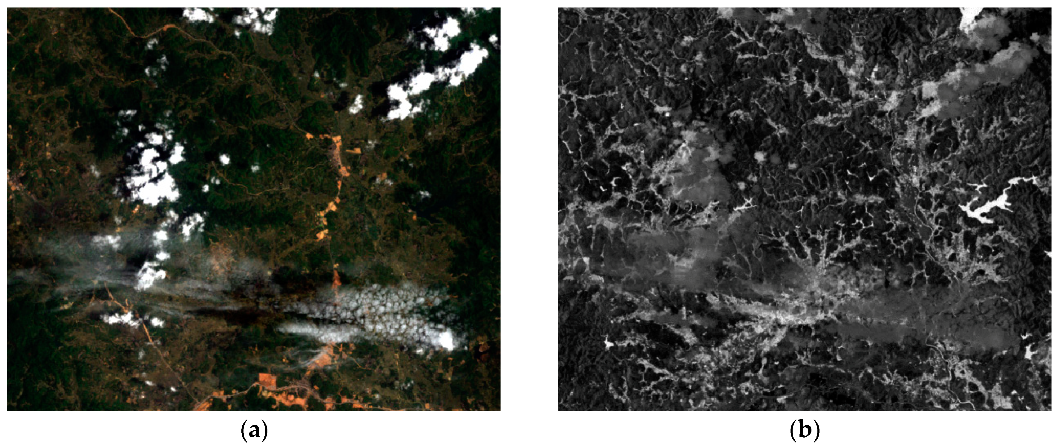
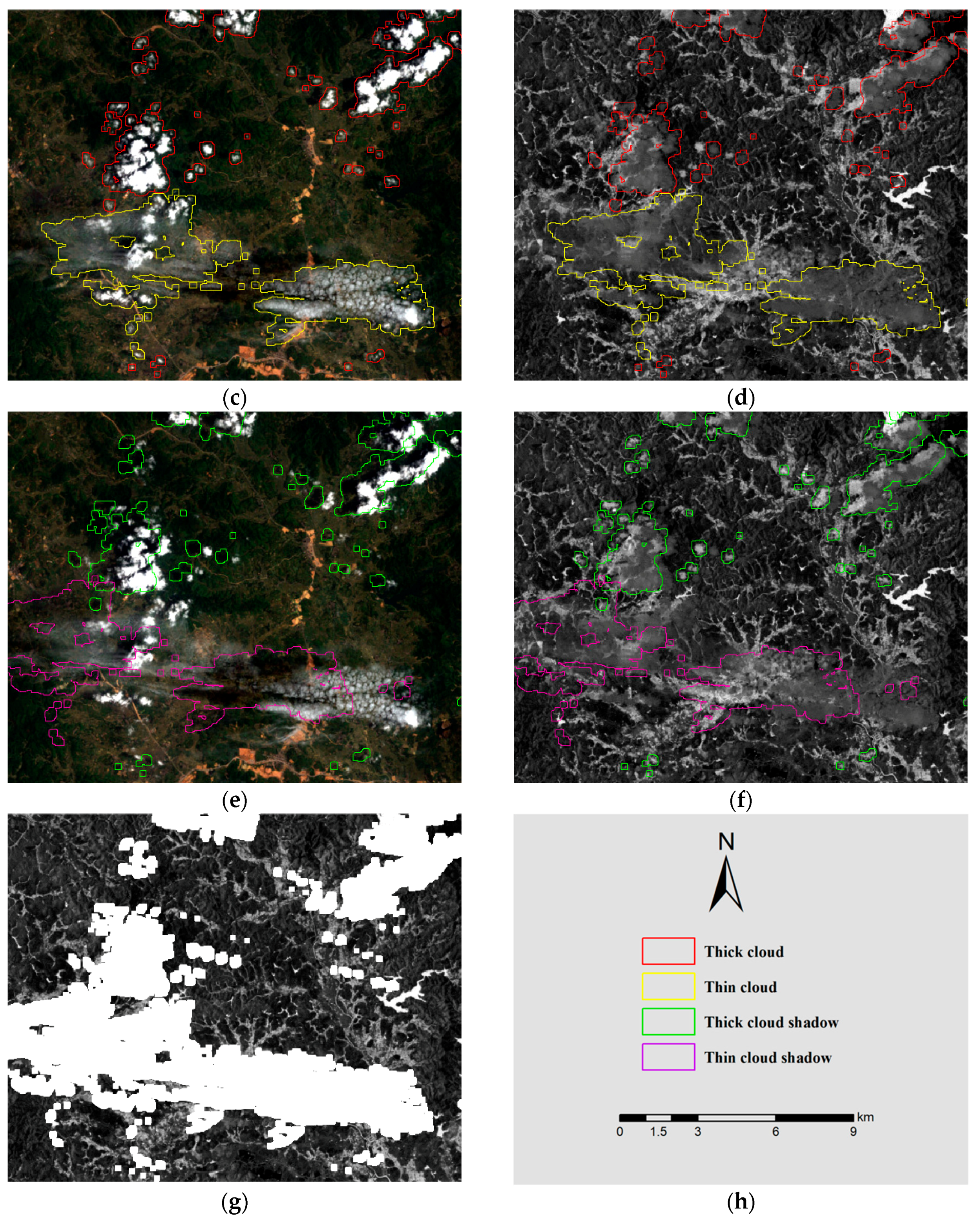
Cloud and cloud shadow masking process. (a) Portion of the Thematic Mapper (TM) True Color scene (after Top of Atmosphere (TOA) processing) of the study area on 21 August 1994. Note that this scene contains two different types of clouds and cloud shadows that produce different relative offsets. (b) is the modified normalized difference water index (MNDWI) of the TOA image. (c,d) are the cloud masks extracted using Fmask in the true color scene and the MNDWI scene respectively. The clouds were visually classified into two types: red for thick clouds and yellow for thin clouds. (e,f) are true color and MNDWI scenes respectively. By moving the relative positions of the two kinds of cloud masks, corresponding cloud shadow masks are generated; the green marks are thick cloud shadows and the purple marks are thin cloud shadows. (g) is the MNDWI scene used for rice extraction after the final removal of cloud and cloud shadows.
Sustainability 10 02570 g002aSustainability 10 02570 g002b
Figure 3. 
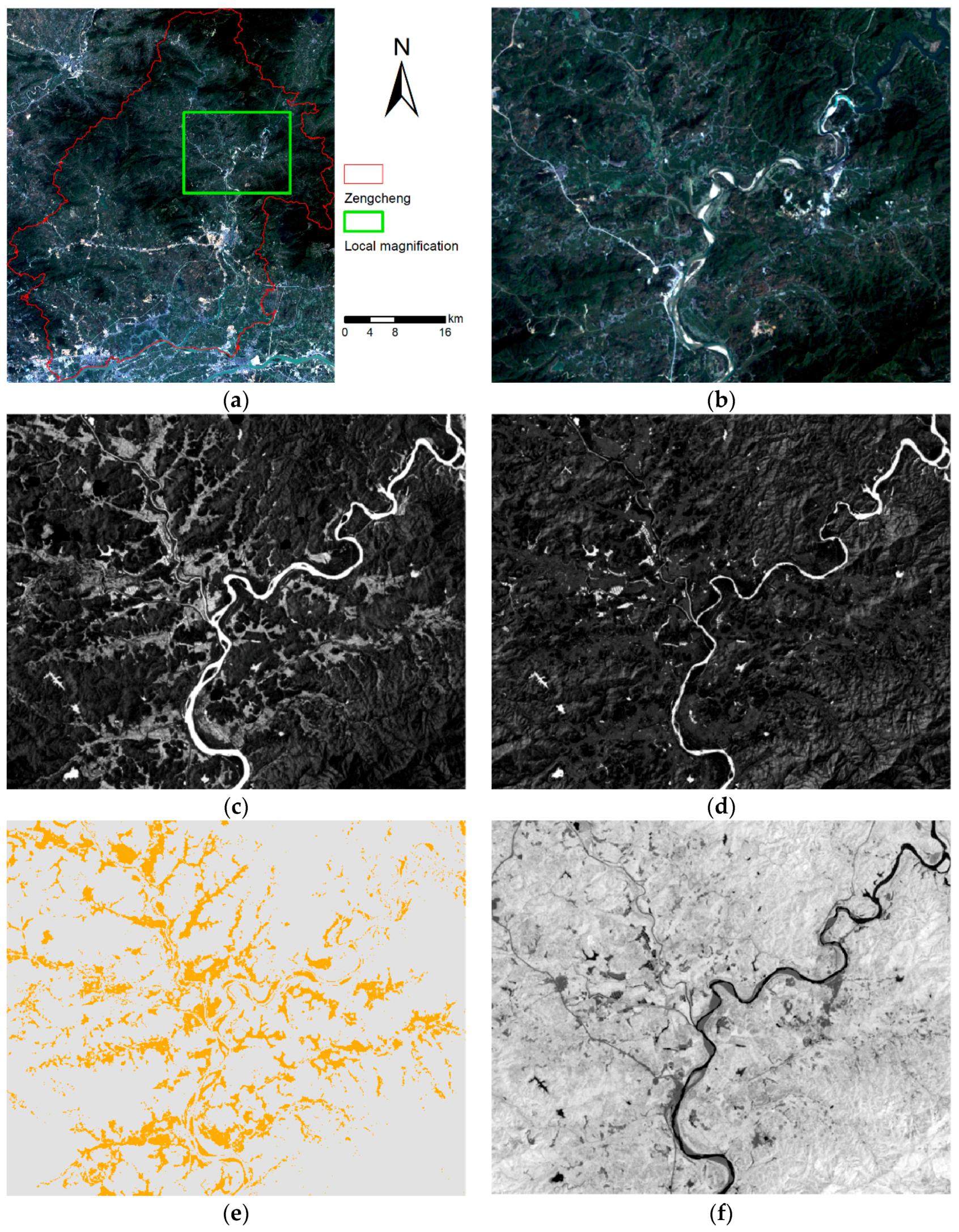
Rice extraction process (1994 as an example). (a) is the true color magnified scene (TOA) of the research area on 24 October 1994. (b) shows a partial enlargement of the study area. (c,d) are the MNDWI scenes on 21 August and 24 October respectively. The yellow parts of scene (e) indicate the flooded areas. In addition to rice fields, the class also includes changes in the river bank. (f,g) are the normalized difference vegetation index (NDVI) scenes on 24 October and 25 November of the current year. The blue parts of scene (h) are the harvested areas. In addition to rice fields, the class also includes other harvested crops. Scene (i) is the overlapping area of the flooded areas and the harvested areas (separated by 96 days), which are the rice planting areas.
Sustainability 10 02570 g003aSustainability 10 02570 g003b
Figure 4. Rice mapping results in the study area (Periods 1, 2, and 3). From period 1 to 3, the scale of rice agriculture in the region dropped sharply by more than 80% and occurred sequentially from south to north.
Sustainability 10 02570 g004
Figure 5. 
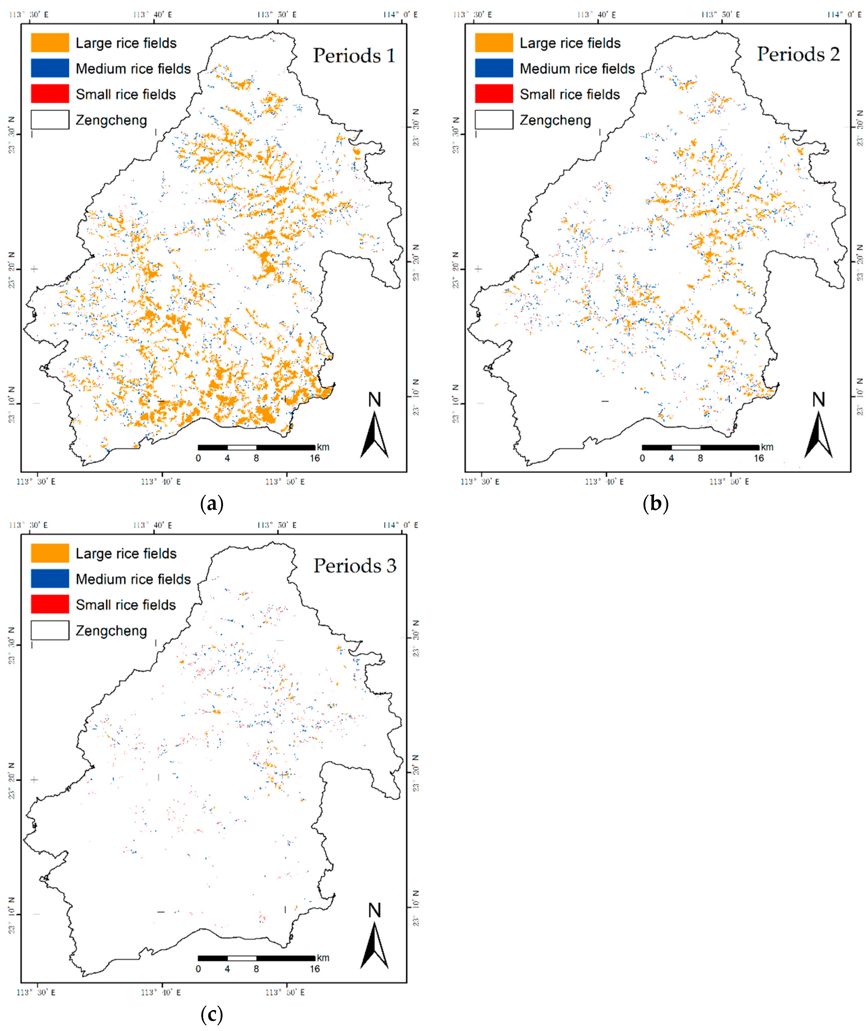
Panicle area of rice in the study area during periods 1, 2, and 3 (small paddy field ≤ 10 Landsat pixels, 11 Landsat pixels < medium paddy field ≤ 50 Landsat pixels, large paddy field > 51 Landsat pixels). From period 1 to period 2, large paddy fields first disappeared in the southern alluvial plains. During the 3rd period, large-scale rice fields were sporadically distributed only in the northern valleys.
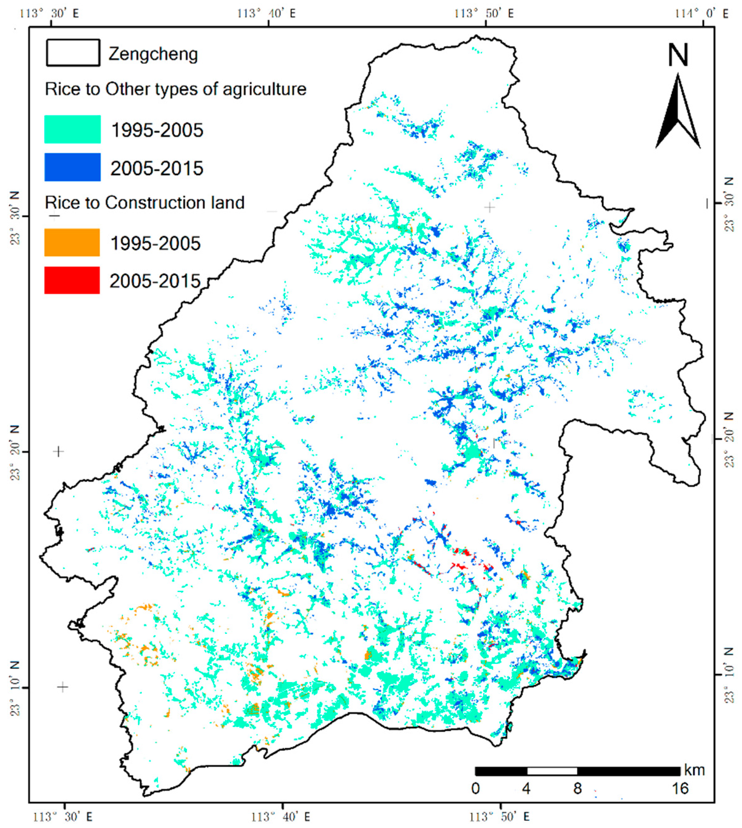
Sustainability 10 02570 g005
Figure 6. Land use change in rice fields in the study area from 1995 to 2015. Only some rice fields have become developed areas in the southern plains. The vast majority of rice fields have been transformed into other agricultural production activities such as growing corn, bananas, sugarcane, and vegetables.
Sustainability 10 02570 g006
Table 1. Social and Economic Details of the Study Area. The GDP was calculated at 1990 prices. (Zengcheng Statistical Yearbook).
YearsGross Agricultural Production (yuan)Gross Domestic Product (yuan)Agricultural PopulationTotal Population
1995   7.40 × 10 8   5.64 × 10 9   5.5 × 10 5   7.2 × 10 5
2005   2.72 × 10 9   2.69 × 10 10   5.8 × 10 5   7.9 × 10 5
2015   4.72 × 10 9   9.46 × 10 10   6.4 × 10 5   8.7 × 10 5
Table 2. Landsat data used in the study. The Landsat images of each year correspond to at least one full rice planting cycle. The early rice planting cycle corresponds to the images covering April to July and the late rice planting cycle corresponds to the images covering August to November.
Time PeriodYearsData Date
Period 1199302/23, 04/04, 05/14, 07/17, 08/18, 09/03, 10/05, 11/22
199407/20, 08/21, 10/08, 10/24, 11/09, 11/25
199603/03, 05/22, 06/07, 07/09, 07/25
Period 2200402/22, 03/09, 05/28, 06/13, 06/29, 07/31, 08/16, 09/01, 10/03, 10/19, 11/04, 11/20
200604/15, 07/21, 08/22, 09/23, 10/25, 11/10
Period 3201308/09, 08/25, 09/10, 09/26, 10/12, 10/28, 11/29
201602/07, 03/26, 07/16, 08/01, 09/18, 10/04, 10/20, 11/05, 11/21
Table 3. The overall, user’s, and producer’s accuracies for the maps of the three periods. The proportional random samples consisting of 200 fields were labeled as either ‘rice’ or ‘non-rice’ for each time point.
Reference Data
ClassRiceNon-riceTotalUser’s Accuracy
Period 1 classified map of rice paddy extentRice9259794.8%
Non-rice89510392.2%
Total100100200
Producer’s accuracy92.0%95.0% 93.5%
Period 2 classified map of rice paddy extentRice832110479.8%
Non-rice17799682.3%
Total100100200
Producer’s accuracy83.0%79.0% 81.0%
Period 3 classified map of rice paddy extentRice8879592.6%
Non-rice129310588.6%
Total100100200
Producer’s accuracy88.0%93.0% 90.5%
Table 4. The overall, user’s, and producer’s accuracies for the maps of the small, medium, and large rice fields in the three periods. A proportional random sample of 300 small rice fields or 200 medium/large rice fields were labeled as either ‘rice’ or ‘non-rice’ for each time point.
Reference Data
TypesClassRiceNon-riceTotalUser’s Accuracy
Period 1 classified map of rice paddySmall rice fieldsRice1132513881.9%
Non-rice3712516277.2%
Total150150300
Producer’s accuracy75.3%83.3% 79.3%
Medium rice fieldsRice901310387.4%
Non-rice10879789.7%
Total100100200
Producer’s accuracy90.0%87.0% 88.5%
Large rice fieldsRice9429697.9%
Non-rice69810494.2%
Total100100200
Producer’s accuracy94.0%98.0% 96.0%
Period 2 classified map of rice paddySmall rice fieldsRice976716459.1%
Non-rice538313661.0%
Total150150300
Producer’s accuracy64.7%55.3% 60.0%
Medium rice fieldsRice822610875.9%
Non-rice18749280.4%
Total100100200
Producer’s accuracy82.0%74.0% 78.0%
Large rice fieldsRice891710684.0%
Non-rice11839488.3%
Total100100200
Producer’s accuracy89.0%83.0% 86.0%
Period 3 classified map of rice paddySmall rice fieldsRice1163715375.8%
Non-rice3411314776.9%
Total150150300
Producer’s accuracy77.3%75.3% 76.3%
Medium rice fieldsRice862210879.6%
Non-rice14789284.8%
Total100100200
Producer’s accuracy86.0%78.0% 82.0%
Large rice fieldsRice95810392.2%
Non-rice5929794.8%
Total100100200
Producer’s accuracy95.0%92.0% 93.5%
Table 5. Comparison of rice paddy areas mapped in this study and from statistical data (rice sown area). The statistical data for period 1 were for the entire area; the statistical data for period 2 were divided into various administrative regions; there were no rice acreage statistical data for period 3.
Data SourcesTotalAlluvial PlainHillsMountains
Rice area in period 1Mapped results (ha)19,542---
Statistical data (ha)22,849---
Rice area in period 2Mapped results (ha)10,217194539674305
Statistical data (ha)14,483276957915923
Table 6. The estimated variance of the overall accuracy, user’s accuracy, and producer’s accuracy for the maps of rice paddies in the three periods. This estimate was performed separately after all pixels had been hard-classified. The first type of hard classification: pixels are rice fields or non-paddy fields. The second type of hard classification: pixels are small rice fields, medium rice fields, large rice fields, or non-rice fields.
ClassEstimated Variance of Overall AccuracyEstimated Variance of User’s AccuracyEstimated Variance of Producer’s Accuracy
Period 1 classified map of rice paddyRice fields0.9180.9260.920
Small rice fields0.7180.7340.763
Medium rice fields0.8950.8770.934
Large rice fields0.9570.9530.960
Period 2 classified map of rice paddyRice fields0.8440.8190.659
Small rice fields0.6360.6070.702
Medium rice fields0.7780.7460.716
Large rice fields0.8920.8730.907
Period 3 classified map of rice paddyRice fields0.8960.8190.720
Small rice fields0.7820.7310.591
Medium rice fields0.8930.8390.767
Large rice fields0.9240.9070.839
Table 7. Industrial output statistics of the study area. The GDP was calculated at 1990 prices (Zengcheng Statistical Yearbook).
YearIndustrial Production (Constant Prices in 1990. Unit: 10,000 yuan)
Alluvial Plain AreaHilly AreaMountains
1995569,026306,56695,938
20053,821,480799,304259,020
20158,224,8143,307,210-

