The Effects of the Cohesion Policy on the Sustainable Development of the Development Regions in Romania

Abstract

The objective of this study was to characterize the development regions in Romania and to measure spatial imbalances, starting from the national and the European Union aspiration to promote more economic and social policies adapted to the different regional particularities. For this purpose, we conducted a multifactorial analysis of the sustainability of the development regions in Romania at NUTS II level by constructing a synthetic index of socio-economic development for the regions that appreciate sustainability and have accepted structural and cohesion funds. The multi-criteria synthetic index was obtained by aggregating several sub-indices (economy, health, education, public utilities, and living standards). We used cluster analysis to identify patterns of regional development in Romania over time. For 1998 and 2006, the same cluster structure was obtained. However, due to economic and social changes that occurred after 2006 (negative impact of the global financial crisis as well as the positive impact of EU funds), in 2016, we recorded another structure of clusters, except in the Bucharest-Ilfov region which continues to present a number of unique features. In addition, we show that the polarized regional development model is increasingly strengthening and the network of urban agglomerations needs to be territorially balanced to boost their ability to “export” wealth.

1. Introduction

A series of challenges cross national, institutional and political borders: globalization, the mobility of the workforce, the climate changes, a strong demographic decline, the importance of the renewable energy sources, etc.

Although some aspects of the EU regional policy are found in the Preamble of the Treaty of Rome, as the recognition of the need to reduce the disparities among the EEC countries and regions, this policy did not reach its current dimension until the end of 1980, thus becoming one of the priority policies in the European Union and replacing its initial objective to reduce the regional economic disparities, measured by GDP/capita, through another wider concept: economic and social cohesion [1]. Consequently, the EU regional policy is one of the key policies in building the European Union and it represents an incentive for national investment programs with co-funding from structural funds [2].

In this context, the cohesion policy was created in a strong relationship with other community policies, for example the competitive policy, the state aid policy, the protection of the environment, in the field of transport, promoting innovation or the development of the informational society. Therefore, we appreciate that the European Union cohesion policy has the possibility to transform the shared challenges for all European Union countries into development opportunities.

The challenge of an integrated approach based on regions for the improvement of the territorial and social cohesion, strongly promoted in the new Cohesion Policy and the European Agenda 2020, strengthens the scientific and technical debate regarding planning tools and practices [3], monitoring/evaluation systems, and governance patterns on a regional and sub-regional level.

Unfortunately, the effects of the previous programming period regarding the intervention by means of structural funds did not always lead to the expected results [4,5,6]. This demonstrates the need to assess the previous actions and to point out new and more efficient solutions [7,8].

This policy acts in very different local contexts and aims at very heterogenous economic and social regional contexts. Even if the cohesion policy has a unique regulation frame, it needs to approach different national and regional circumstances including various institutional arrangements. Moreover, its operations include a multitude of measures and rules as well as national, regional and local systems [9].

The main objective of our research was: to illustrate the effects of economic integration and the implementation of cohesion policy on the development regions of Romania; to perform multi-criteria hierarchy of regions; and to measure the development gaps between them. The selected research period allowed us to provide information on the stage of economic and social development prior to joining the European Union (2006) and to determine the evolutions that the development regions have had until the end of 2016, given that they had benefited from the Structural and Cohesion Funds related to the 2007–2013 programming period. In addition, we found the patterns of development of the regions over time through cluster analysis, including the synthetic index of socio-human development as determined in our research.

2. Literature Review

According to the conceptual frame and to some key methodological choices, different studies reached contradictory conclusions [10]. The existing research, based on tradition regression methods indicates that the benefits of this policy are fully maximized only in the regions with pre-existing socio-economic conditions and/or when they benefit from the ability to implement favorable policies. In exchange, with some exceptions [11,12], the existing counterfactual analysis tries to outline the “net” impact of a policy at the EU level ignoring the heterogeneity potential of the regions in the regression analysis.

In the same context, other authors [13] proposed to build a synthetic indicator which should allow the measuring of the progress registered with the economic and social cohesion policy from the regions of Spain and Portugal in the EU regional policy.

At the same time, European Union Member States are characterized by a significant variation regarding the level of sustainable development. The disparities in this field can have a negative effect on the national economies. In this sense, the European Union elaborated methods for the continuous monitoring of progress to accomplish a sustainable development for member states based on some indices regarding the following aspects: the socio-economic development, consumption and production, social inclusion, demographic changes, public health, climate and energy changes, sustainable transport, natural resources, global partnership, and governance (report regarding the analysis of the innovation 2011) [2]. These methods are based on analysis and evaluation of diversified indicators. Sustainable development indicators are used to monitor the implementation of the sustainable development strategy in a report published by Eurostat every two years. From more than 100 indices, eleven have been identified as main indicators. The purpose of these indicators is to present global progress towards sustainable development correlated with the objectives defined in the directives [14]. In addition to these sub-indicators, other synthetic indicators with a more general character have been elaborated. The synthetic indicators describe and measure the processes which represent the quality of life of the population and its impact on the economy and the environment. These synthetic indicators can include sustainable development, environment performance, economic welfare, and environmentally sustainable development indicators, among others.

Currently, the economic dimension of sustainable development is a major problem and is an important trend of economic research [15,16,17]. Sustainable development concerns achieving balance in three main dimensions at once: in the economic dimension signifying the pursuit of sustainable economic development; in the social dimension signifying the protection of public health and social integration; and in the environmental dimension placing a significant emphasis on environmental protection and natural resources in a way as not to endanger the capabilities to meet the needs of future generations [18,19].

There are several comparative analyses in the field of sustainable development of the EU Member States. Venkatesh used the total sustainability index to compare the development of twelve Asian countries [20]. Bujnowicz-Haras et al. evaluated the level of sustainable development of the European Union countries using taxonomy methods under the form of the Hellwing development model based on 23 variables grouped into themes: socio-economic development, consumption and production, social inclusion, demographic changes, public health, climate changes and energy, and natural resources [21]. Zelazna and Gołebiowska performed studies on the monitoring indicators especially on the greenhouse gases, on the shares of the renewable energy in the final gross energy consumption and the primary energy consumption [22]. Stec et al. carried out social-economic evaluation of the aspects related to sustainable development in the EU Member States using 27 variables divided into four groups: the demographic potential and the labor market, the economic potential, the development level of the social infrastructure and the development level of the technical infrastructure [23].

Other authors [24] proposed a relative evaluation for the sustainability level of the EU Member States using the aggregate indicator for the relative sustainability level covering ten diagnosis variables characterizing the sustainable development of the EU Member States. Comparative analysis was carried out based on the linear classification of the countries according to the aggregate indicator and based on the volatility index.

The member countries of the European Union are characterized by a significant variation on the level of sustainable development. Disparities in this area can adversely affect the functioning of the economic system [25]. Other authors [26] used a method of normalization of values different from the one normally used in multi-criteria evaluations to determine the economic development of individual regions. This allowed the determination of unused potential of economic development in each region.

On the other hand, the problem of regional disparities is a matter of special interest both as a decisive factor and for practitioners and university teaching staff [27]. In Romania, one of the main priorities of the economic policy is “the balanced and sustainable territorial development of the regions in Romania”, as well as the “reduction of the economic and social disparities between Romania and the other EU Member States” [28].

Fotea and Guțu [29] emphasized that, due to their endless resources, large scale influence and social, cultural and economic involvement, higher education institutions have played a decisive role in the development of societies. The accelerated socio-economic transformations, especially in the last decades, often encompassed in concepts such as “knowledge society” or “knowledge-based economy”, show the great importance of knowledge in the process of economic growth and development.

Unfortunately, most empirical studies carried out in Romania pointed out a waring process of deepening the regional disparities started from the transition period and continuing up to now [30,31,32,33,34,35]. Despite the availability of structural funds and significant cohesion funds which should enhance the economic development for the underdeveloped regions, the EU accession did not counteract the disparities for the regional based growth. On the contrary, the developed regions obtained the largest part of the post-accession benefits, based on their expertise in accessing European funds [36,37]. These discrepancies are highly visible considering foreign direct investments, which are concentrated in the region Bucharest-Ilfov [38]. Another aggravating factor for the territorial disparities was the recent economic crisis which had unequal effects at the regional level [39,40].

Much of the literature on regional disparities is focused on the analysis of the GFP per capita indicator, as a complex economic measure for the development level [33,34,35,36,37,38,39,40,41]. In addition, other studies used regional GDP to highlight the disparities between development regions [42,43].

At the same time, another important contribution [44] is research considering a more complex approach to regional disparities based on more indicators offering complementary information. This paper points out the problem of the territorial convergence in Romania, combining the economic and social perspectives by using a new synthetic development indicator at a county level. The index includes various economic and social aspects (GDP/capita, labor productivity and life expectancy), offering a synthetic development measure that is used in assessing the degree of convergence in the counties of Romania.

However, the above-mentioned methodologies do not cover the matter and only confirm that there is a universal quantification method including various aspects of sustainable development.

Starting from these elements, our study aimed at researching the phenomenon of regionalization, of the cohesion policy and of the effects of putting this in practice in Romania to find suitable solutions for Romania to increase its capacity, develop sustainably and benefit from structural and cohesion funds in nominal as well as economic and social development terms.

In our process, we used a cluster of research methods to better outline the phenomenon of regional sustainable development in Romania and its implications. Therefore, in our research, we performed comparison, benchmarking, synthesis and cluster analyses to identify some development patterns of the regions in time.

3. Materials and Methods

In our research, we started from the Global Index Method for Regional Development, developed and adapted by a research committee from the Bucharest Academy of Economic Studies [45], holding that there is a wide range of criteria and indicators for the analysis of the economic and social development level on regions. The evaluation of territorial disparities is often limited to pointing out the information related to a single economic or social indicator, thus we assess that using various indicators would lead to different perspectives sometimes opposed, on the same territorial disparities. This shortcoming can be avoided by using a method based multiple criteria of evaluation; for example, the calculation of the regional synthetic indicators allows us to capture several economic and social aspects, both quantitative and qualitative related to the regional development.

Therefore, we considered X₁, X₂, … X_p to be the analyzed indicators used to outline the development level of the n regions in Romania. Firstly, we calculated using the normalization procedure (the minimum–maximum method) the adjusted values of the indicators for each region using Equation (1):

$$I_n^m=\frac{X_n^m-X_{\min }^m}{X_{\max }^m-X_{\min }^m}$$

(1)

where $X_n^m$ is the value for the indicator m for the n region, and $X_{\min }^n$ and $X_{\max }^m$ represent the minimum and maximum value of the m index, respectively.

When using indicators with a negative significance (for example, the mortality rate and the unemployment rate), the adjusted values of the indicator are determined by means of Equation (2):

$$I_n^m=\frac{X_{\max }^m-X_n^m}{X_{\max }^m-X_{\min }^m}$$

(2)

The purpose of using this method was to obtain a uniform variation of the indicators, having values between 0 and 1, irrespective of the type of the index and of the margin which was initially registered.

Next, we determined the Global Development Index for each n region by calculating a simple or weighted average (Equation (3)) of the values which were previously adjusted:

$$I^n=\frac{1}{p}{\displaystyle \sum _{m=1}^p{I}_n^m}$$

(3)

This method has several advantages that can point out territorial differences because it assesses more different variables, considering the indicators included in the evaluation have a different importance and offer the possibility to allocate in the calculation of the final average, various shares for the adjusted value according to the importance we give them in the territorial analysis carried out.

4. Results

4.1. Building the Synthetic Index for the Economic and Social Development of the Regions: Assessment Tool for the Effects of Regionalization and Attracting Structural and Cohesion Funds in Romania at the NUTS II Level

Starting from the Global Development Index, we built a territorial synthetic index considered to be more adapted to the development particularities for the regions in Romania. We created this indicator with criteria that should allow obtaining information based on the data available in the official statistics. To build the multi-criteria indicator for the economic-social development of the regions in Romania [43], we performed following steps:

Step 1.

We selected the researched period so that the result of the analysis reflects the level of the existing disparities for the division of the Romanian territory in the current structure, in eight development regions (1998) should include relevant information regarding the socio-economic development stage before the accession to the European Union (2006) and should point out the evolution of the development regions in the programming period 2007–2013, when they benefited from structural and cohesion funds.

Step 2.

We chose the social and economic indicators as the object of research describing the size of the disparities among regions and we created a hierarchy of the territorial units. First, we identified the significant indicators from the perspective of the more complex characterization of the territorial differences. Our option for the chosen indicators was based on the desire present various degrees of economic and social development but was restricted by the available data on regions from the official statistics. Therefore, we chose 16 indicators, selected based on the relevance and the availability of the official data, avoiding redundancies.

The chosen indicators were structured into five classes (the statistical data being on the level of the region). We considered the following structure:

Class 1, Economy: We considered the essential elements related to the economic development of the development regions:

• Gross internal product/capital, expressed in thousands of RON/capita;
• Average monthly net income, expressed in RON/employee;
• Registered unemployment rate, expressed in percentages.

Class 2, Health: We considered relevant the following indicators:

• The number of hospital beds, expressed in beds/1000 inhabitants of the region;
• The number of doctors per 1000 inhabitants expressed in doctors/1000 inhabitants of the region;
• Infantile mortality rate, deaths under one year per 1000 newborns;
• The average life expectancy at birth, expressed in years.

Class 3, Education: we chose to include the indicators:

• The rate of school dropout in the pre-university education, expressed in percentages;
• The total number of students, expressed by a total number of students per 1000 inhabitants.

Class 4, Public Utilities: We included the following:

• The density of the town street on development regions, expressed in km/100 kmp;
• The density of the sewage system expressed in km/100 kmp;
• The surface of green places in cities and towns as a percentage from the build-up areas from towns in the development regions.

Class 5, Living Standard: We included indicators regarding:

• The living surface of the housing fund, expressed in mp/inhabitant;
• The volume of natural gases distributed, expressed in mc/inhabitant;
• The quantity of drinking water distributed on inhabitant expressed in mc/inhabitant;
• The criminality rate expressed in people with a final conviction per 100,000 inhabitants.

We chose these indicators considering that the investment in the analyzed period 1998–2016, both from national funds and from structure and cohesion funds, could determine significant changes and high differences on the development level in our country. We considered that these differences can be shown through the five classes of indicators included in our study. We noticed that, for some indicators, such as the incomes from salary, the average life expectancy and the infantile mortality rate, the positions of the different regions are pretty close, while, for some other indicators, such as the development level for public utilities, there are big differences, because of both the influence of the surface and the population and some specific condition for each area.

Step 3.

We carried out the calculation of some indicators derived based on the primary ones, so that we obtain a better comparison level among regions. To carry out relevant comparisons, we considered appropriate the transformation of the primary indicators as they are described by the National Institute of Statistics into a new form, according to the population of the region or to the surface of the region and the primary indicator.

In this way, by showing the density of town streets, the density of the sewage pipes and the density of the green places, we reported the primary indicators to the surface of that regions. From the data regarding GDP, the hospital beds, the number of medical staff, the number of students for each region, the natural gases distributed and the volume of drinking water, per capita indicators were derived.

Step 4.

We carried out the standardization of the primary data, because the chosen indicators for the calculation of the synthetic index for the economic-social development have different measurement units (RON, percentages, different values per 100 km², per 100,000 people, etc.) and register different variation margins and different changing means making it impossible to compare them or to aggregate them directly. The conversion the primary indicators into a common measurement unit and a form that should facilitate the aggregation of the values on the regional level was made through the minimum–maximum standardization method. With the help of this method, we calculated the standard value in two ways.

For those indicators showing a more favorable situation when values are higher (e.g., GDP/capita, the number of students per 1000, inhabitants etc.), we calculated the standard value between 0 and 1 for each of the indicators using the Equation (4):

$$y_{nm}=\frac{x_{nm}-\min (x_m)}{\max (x_m)-\min (x_m)}$$

(4)

where $y_{nm}$ is the standar value of the m indicator for the n region (n = $\overline{1,8}$ and m = $\overline{1,9}$ and $x_{nm}$ is the primary value of the m indicator for the n region.

For those indicators showing a better situation when values are lower (e.g., the unemployment rate and the criminality rate), we applied Equation (5):

$$y_{nm}=\frac{\max (x_m)-x_{nm}}{\max (x_m)-\min (x_m)}$$

(5)

We thought these changes are necessary to accomplish a unitary evaluation which should not rely on the nature of the sub-indicators or on their different measurement units. By means of this standardization, the region with the highest territorial performance for a certain indicator registers the value 1, while the region with the lowest performance will have the standardized value 0.

Step 5.

For each “n” region and for each “c” class of indicators, we calculated sub-index (class) $I_c^n$, creating a simple arithmetic average for the standardized values of the class indicators:

$$I_c^n=\frac{1}{p_c}{\displaystyle \sum }_{m=1}^{p_c}{y}_m^n$$

(6)

where n = $\overline{1,8}$; m = $\overline{1,p_c}$; and p_c is the number of characteristics included in the c class.

By synthesizing the standardized values and building a sub-index for each class, we obtained useful information to point out the disparities and to create a partial hierarchy of the region according to various criteria.

Separate analyses of the disparities for each of the three components of the sub-index for the class Economy in 1998, 2006 and 2016 bring valuable information (

Table 1. Sub-index for the class ECONOMY for 1998, 2006 and 2016 *.

	1998	2006	2016
Region NORTH-WEST	0.275693979	0.299201648	0.398858035
Region CENTER	0.336792583	0.167104663	0.335990155
Region NORTH EAST	0	0.220588235	0.333333333
Region SOUTH EAST	0.386877422	0.194714622	0.119242773
Region SOUTH-MUNTENIA	0.213253846	0.105624421	0.16577885
Region BUCHAREST-ILFOV	1	1	0.923076923
Region SOUTH WEST OLTENIA	0.502122575	0.251973316	0.02923208
Region WEST	0.37713764	0.378881859	0.426471387

Source: calculations performed by the authors based on the date from INSSE Tempo-online. * GDP/regional inhabitant is expressed on the level of the year 2014.

). From the perspective GDP per capita, which is the most relevant indicator of the economic development level, the region North East registers the lowest value for this indicator, followed closely by the region South West Oltenia. The region North East includes some of the counties with the lowest development in Romania: Vaslui is last place in the territorial hierarchies, followed by Botoșani, Neamț and Suceava.

A comparable situation can be noticed in the case of the monthly average salary, where the Region North East is among the lowest together with the region South East. As for the unemployment rates, the highest disparities were registered in the regions South West, Oltenia and South East.

The amplitude of the disparities is maintained when we look at it from the perspective of the sub-class index which reunites the three components by aggregating the sub-indicators, as the individual variations are not reduced.

In the class of indicator Health, we notice a deepening of the disparities in the analyzed period, especially in the regions South East and South Muntenia. The indicator life expectancy at birth has a low variation due to the multitude of factors influencing it. The infant mortality rate, used to assess the evolution of the interregional disparities under the aspect of the health level, has the same evolution with the indicators the number of hospital beds per 1000 inhabitants and the number of doctors per 1000 inhabitants.

Even though the infantile mortality rate was reduced between 1998 and 2016, this indicator has not improved enough to take Romania from the maximum negative position registered on the level of the European Union. The disparity among the urban and rural values of the index is maintained at approximatively 4–5 in this period. Despite the improvement of the living standard, the existing disparities between the village and the town are still in favor of the town. In the European Union, these differences have reduced, while, in Romania, they remain constant. This trend is also valid for the level of life expectancy. For the male population, it is constantly higher, with almost two years in the urban environment as compared to the rural environment and with almost one more year for women from towns as compared to women living in the countryside. In Romania, there is a strong social stratification determined by the profile of the living space. This stratification is present not only in the quality of living but also in the life expectancy (

Table 2. Sub-index for the class HEALTH for 1998, 2006 and 2016.

	1998	2006	2016
Region NORTH-WEST	0.377277963	0.262868865	0.299191166
Region CENTER	0.587692014	0.404985298	0.37275608
Region NORTH EAST	0.18590952	0.195187769	0.173608189
Region SOUTH EAST	0.327923903	0.21394552	0.065825206
Region SOUTH-MUNTENIA	0.215490898	0.081389694	0.08186892
Region BUCHAREST-ILFOV	0.899331178	0.999806723	0.999651387
Region SOUTH WEST OLTENIA	0.311279614	0.161301264	0.259999531
Region WEST	0.680946816	0.349369515	0.37447155

Source: calculations carried out by authors based on the data INSSE Tempo-online.

).

If we refer to the aspects related to education (

Table 3. Sub-index for the class EDUCATION for 1998, 2006 and 2016.

	1998	2006	2016
Region NORTH-WEST	0.299143793	0.304419914	0.274882645
Region CENTER	0.316899588	0.385647085	0.158348949
Region NORTH EAST	0.508587037	0.509577589	0.323099435
Region SOUTH EAST	0.180120811	0.179748017	0.228635397
Region SOUTH-MUNTENIA	0.955315215	1.000146572	0.799947473
Region BUCHAREST-ILFOV	0.524355224	0.378594125	0.500034404
Region SOUTH WEST OLTENIA	0.170348027	0.115006822	0.14617221
Region WEST	0.244692146	0.221836454	0.442625277

Source: calculations carried out by authors based on the data INSSE Tempo-online.

), regarding the rate of school dropout and the number of students from each region, we must point out that the investment in education does not necessarily lead to high regional development. To obtain such a result, it is necessary, in addition to having good values of these indicators, to create the conditions for good employment and standard of living, to enhance local stability and reduce outmigration of persons with a high educational level. Therefore, investments in education is not successful when highly qualified staff migrate from the country for better working conditions and/or due higher incomes.

For the indicators from the class Public Utilities (

Table 4. Sub-index for the class PUBLIC UTILITIES for 1998, 2006 and 2016.

	1998	2006	2016
Region NORTH-WEST	0.03124341	0.024311087	0.171770861
Region CENTER	0.00840538	0.095122391	0.15966504
Region NORTH EAST	0.243178709	0.321716982	0.315194654
Region SOUTH EAST	0.194908853	0.460167454	0.573060017
Region SOUTH-MUNTENIA	0.101601026	0.238845837	0.159611244
Region BUCHAREST-ILFOV	1.000061956	1.000125615	1.000000016
Region SOUTH WEST OLTENIA	0.224913997	0.201508056	0.192459037
Region WEST	0.178881154	0.369472707	0.486180569

Source: calculations carried out by authors based on the data INSSE Tempo-online.

), there is a very high variability, both because of the influence of the surface of the regions and of the population, as well as due to some specific conditions for each region.

We noticed very high territorial disparities for the indicators: the density of green spaces in cities and towns, the density of public sewage system, and the density of the town streets. These territorial variations of the indicators are mostly explained as the municipality of Bucharest has a smaller surface as compared to the other regions but also a higher population density and a good network of public utilities (

Table 5. The sub-index for the class LIVING STANDARD for 1998, 2006 and 2016.

	1998	2006	2016
Region NORTH-WEST	0.337244216	0.323489109	0.341337655
Region CENTER	0.629367495	0.523618992	0.456098427
Region NORTH EAST	0.032884771	0.022472193	0.138992087
Region SOUTH EAST	0.279554254	0.263715566	0.322549687
Region SOUTH-MUNTENIA	0.314990218	0.382643859	0.217261157
Region BUCHAREST-ILFOV	0.807043117	0.944909995	0.970828124
Region SOUTH WEST OLTENIA	0.144386857	0.306699988	0.262162301
Region WEST	0.432930277	0.430181368	0.425997351

Source: calculations carried out by authors based on the data INSSE Tempo-online.

). All standardized indicators resulted from the report of the surface of the regions are influenced by this characteristic.

The major dimension of structure or the existence of regional disparities are strongly influenced by the urban–rural axis, by the phenomenon of residential concentration, and the access to services and infrastructure.

Step 6.

We carried out the aggregation of the Sub-indicators $I_c^n$, for each territorial unit n under the form of a weighted average (Equation (7)). The The share (p_c) given for each class c takes into account the relative significance of the indicators relating to the respective class, reported to the other classes of indicators, so that if we sum up the share we obtain 100%:

$${\displaystyle \sum _{c=1}^5{p}_c}=100\%$$

(7)

Considering the relevance of the indicators and the importance of the different economic, social aspects and the utilities they reflect, we considered adequate the aggregation of the sub-indicators granting the classes considered in our study the following different shares:

• Class 1, Economy—40%
• Class 2, Health—15%
• Class 3, Education—15%
• Class 4, Public Utilities—15%
• Class 5, Living Standard—15%

We calculated the Synthetic indicator for economic-social development (

Table 6. Synthetic index of economic-social development for 1998, 2006 and 2016.

Synthetic Index	1998		2006		2016
	Size	Position	Size	Position	Size	Position
Region NORTH-WEST	0.267013999	7	0.256944005	5	0.322620563	3
Region CENTER	0.366071705	3	0.27824793	4	0.306426336	4
Region NORTH EAST	0.145584006	8	0.245578474	6	0.275967488	5
Region SOUTH EAST	0.302127142	6	0.245522332	7	0.226207655	7
Region SOUTH-MUNTENIA	0.323411142	5	0.297703663	3	0.255114859	6
Region BUCHAREST-ILFOV	0.884618721	1	0.898515469	1	0.889807859	1
Region SOUTH WEST OLTENIA	0.328488304	4	0.218466746	8	0.140811794	8
Region WEST	0.381472615	2	0.35718175	2	0.429979767	2

Source: calculations carried out by authors based on the data INSSE Tempo-online.

) for each region n (I_n) by aggregating the sub-indicators p (class) under the form of a weighted arithmetic share:

$$I_i=\frac{{\displaystyle \sum _{c=1}^5{I}_c^n}}{100},\mathrm{i}=\overline{1,n}$$

(8)

Step 7.

Based on the aggregation of the partial class indicators and of their weighting, we carried out for each of the analyzed years in our study a ranking of the development regions, starting from the highest value, which points out the less favorable situation. In this classification, the value of the calculated indicator for the territorial disparities from the point of view of the economic-social development is between 1 (being the best score) and 0 (if the same region registered the lowest level for all primary indicators).

The synthetic indicator for the economic-social development was calculated based on several criteria so that the results obtained should allow the complex evaluation of the relative positions of the regions, based on a series of features structured in classes of similar indicators. We opted for this method because, besides showing the territorial imbalances, it facilitates the multi-criteria hierarchy of the regions and the measurement of the development disparities among these. Moreover, the selected research period allowed us to outline information regarding the economic-social development stage before the European Union accession (2006) and to find the evolution of the development regions up to the end of 2016, because they benefited from structural and cohesion funds for the programming period 2007–2013.

The variation registered by the index on development regions shows the fact that the less developed regions in Romania are concentrated in the North-East, Câmpia Româna, South-West Oltenia, and South Muntenia regions, while the more developed regions are especially in the west and in the center of the country. An exception is the region Bucharest-Ilfov, which dominates the classifications and its classification was significantly enhanced by the amplitude of the territorial disparities.

It is interesting to note that the multi-criteria analysis points out different results from those of a unifactorial analysis: the hierarchy of the regions based on the synthetic index places the region South West Oltenia in the last place, while the hierarchy of the regions based on GDP/capita places the North East region in last place (

Table 7. The hierarchy of the development regions based on the synthetic index and on GDP/capita.

	Macroregion One		Macroregion Two		Macroregion Three		Macroregion Four
	North West	Center	North East	South East	South Muntenia	Bucharest-Ilfov	South West Oltenia	West
Position calculated based on the synthetic index	3	4	5	7	6	1	8	2
Position calculated as a share from GDP/place average	6	3	8	4	5	1	7	2

Source: calculations carried out by authors based on the data INSSE Tempo-online. GDP/regional capita expressed on the level of the year 2014.

).

In the evolution of the synthetic development index, we notice that the regions Bucharest-Ilfov and Centre have a special situation: they keep their position in the regional hierarchy, especially for the economic development. The region South West Oltenia registered a very unfavourable evolution, from position 4 in 1998 to the last in 2016. The region has a high rurality degree being confronted with a massive migration of the workforce on a high unemployment level background.

4.2. Applying the Cluster Analysis on the Development Regions of Romania

Continuing the multifactorial analysis of the effects of economic integration and of implementing the cohesion policy on the development regions in Romania, we propose the use of cluster analysis to identify some development patterns for the regions in time.

The cluster analysis aims, in a series of data, to identify groups (clusters) with similar elements inside a group and with special elements if these elements belong to another group. Cluster analysis offers the possibility to analyze the similarities and differences of elements to classify them into different homogenous classes. Each variable from the set of analyzed data is assigned to a group and the multitude of groups is a discrete and non-classifiable cluster.

To reach the objective of the analysis, we chose the series of data corresponding to the five variables included in the analysis (

Table 8. List of analyzed variables.

GDP	Gross Domestic Product per Capita, Current Prices
SISHD	Synthetic index of social-human development
FDI	Foreign direct investments
UEMPR	Unemployment rate
CEMP	Civil employed population

Source: calculations carried out by authors based on the data INSSE Tempo-online and NBR data.

) and to the eight development regions of Romania. The analysis started from the idea that the determining factor for the development level of a region is the Gross Domestic Product per capita. Among the factors with a major influence on the development level, there are the foreign direct investments, the unemployment rate and the number of civil employees. At the same time, we introduced in the cluster analysis the synthetic index for the socio-human development, as calculated in the previous section.

Starting from these aspects, the matrix resulted Y = ${\Vert y_{ij}\Vert }_{i=\overline{1,n}}$, ${}_{j=\overline{1.m}}$ where m = 5 represents the number of variables and n = 8 corresponding to the number of development regions. We transformed it (the method z-score):

$$z_{ij}=\frac{y_{ij}-\overline{y_j}}{{\sigma }_j},\mathrm{where}\overline{y_j}=\frac{{\displaystyle {\sum }_{i=1}^n{y}_{ij}}}{n},{\sigma }_j=\sqrt{\frac{{\displaystyle {\sum }_{i=1}^n{(y_{ij}-\overline{y_j})}^2}}{n-1}}$$

(9)

to generate the proximity matrix (W = ${\Vert w_{ij}\Vert }_{i=\overline{1,n}}$, ${}_{j=\overline{1,n}}$). Then, we used the Euclidean distance formula [46]:

$$\begin{array}{l}\mathrm{W}={\Vert w_{ij}\Vert }_{i=\overline{1,n}},{}_{j=\overline{1,n}},w_{ij}=\sqrt{{\displaystyle {\sum }_{i=1}^n{(z_{ik}-z_{ij})}^2}},\\ \mathrm{j}=\overline{1,m},\mathrm{k}=\overline{1,m},\mathrm{j}\ne i,\mathrm{k}\ne i,w_{ii}=0\end{array}$$

(10)

Subsequently, for the determination of the distance among clusters, we used the Wards Method, [47]:

$$\Delta (A,B)={{\displaystyle \sum _{i\in A\cup B}\Vert x_i^{}-m_{A\cup B}\Vert }}^2-{{\displaystyle \sum _{i\in A}\Vert x_i-m_A\Vert }}^2-{\displaystyle \sum _{i\in B}\Vert x_i}$$

(11)

To test the significance of the belonging of the five variables to the clusters, we used ANOVA (analysis of variance). The condition of applying this is that the dispersions of the analyzed variables should not differ significantly. To test the fulfilment of this condition, we used Levene’s Test whose hypothesis is null:

$$H_{0\_1}:{\sigma }_1^2={\sigma }_2^2={\sigma }_3^2=\mathrm{\dots }={\sigma }_r^2$$

(12)

The condition of accepting the null hypothesis H_{0_1} is:

$$\mathrm{Sig}.\mathrm{F}>\alpha \mathrm{equivalent}\mathrm{to}{F}_{stat}<F_{\alpha ,r-1,n-r}$$

(13)

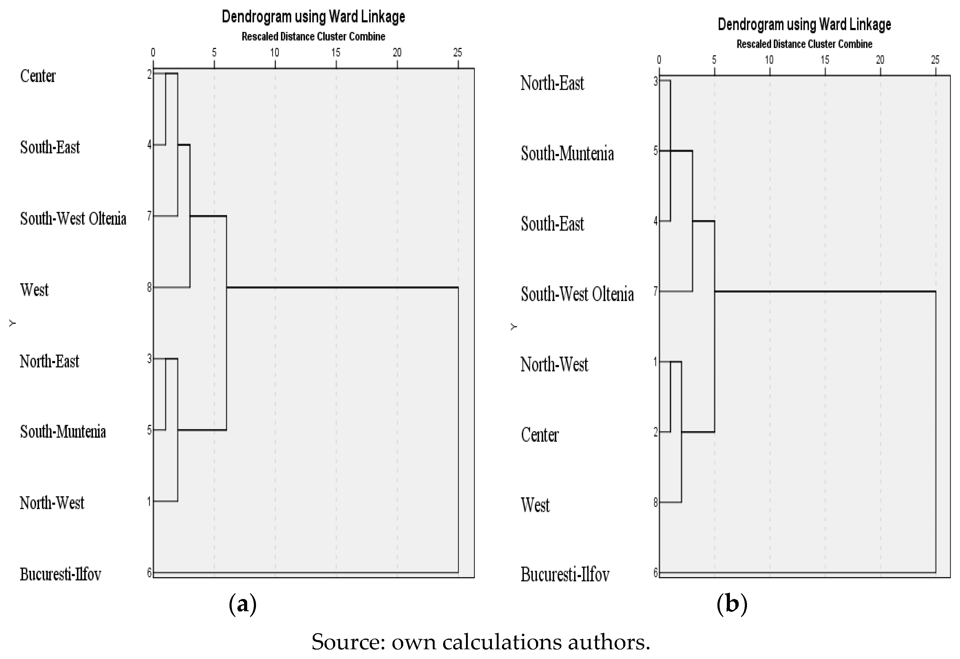
Applying the Hierarchical Cluster Analysis Method for the series of data corresponding to 1998, 2006 and 2016, we obtained the dendrograms presented in Figure 1.

The three years included in the analysis resulted in three clusters (

Table 9. The structures of the clusters on the level of 1998, 2006 and 2016.

Analyzed Year	Cluster	Development Regions
1998	A	North East, South Muntenia, North West
	B	Centre, South East, South West Oltenia, West
2006	C	Bucharest-Ilfov
2016	A	North West, Center, West
	B	North East, South Muntenia, South East, South West Oltenia
	C	Bucharest-Ilfov

Source: own calculations.

), from which one has one developed region, the region Bucharest-Ilfov. At the same time, we pointed out that, for 1998 and 2006, there was the same structure of the clusters. Due to the economic and social transformations after 2006 (the negative influence of the global economic and financial crisis as well as the positive influence of the European funds), in 2016, there was registered another structure of the clusters in addition to the developed region Bucharest-Ilfov which continues to present a series of unique characteristics.

Applying the Levene’s Test on the series of data corresponding to each year the analysis was carried out resulted in the null hypothesis being accepted (

Table 10. Results of the test of homogeneity of variances for 95% level of trust.

Year	1998		2006		2016
Variables	Levene’s Statistic *	Sig.	Levene’s Statistic *	Sig.	Levene’s Statistic *	Sig.
GDP	0.100	0.765	0.209	0.667	0.313	0.600
SISHD	3.205	0.133	1.142	0.334	0.163	0.703
FDI	0.127	0.736	0.061	0.815	0.548	0.493
UEMPR	2.116	0.087	0.502	0.510	0.001	0.982
CEMP	0.457	0.529	1.375	0.258	0.015	0.906

* Groups with a sole case are ignored in the calculation of the test of homogeneity of variances. Source: own calculations using SPSS.

). This conclusion results from the fact that all values are significant (α = 0.05). Consequently, to test the significance of belonging of the five variables to clusters, the ANOVA methodology can be used.

The results of using the ANOVA methodology (

Table 11. Results of using the ANOVA methodology for 95% level of trust.

Null Hypothesis: The Averages of the Variables on the Level of the Cluster are not Significantly Different
Year	1998		2006		2016
Variable	F	Sig.	F	Sig.	F	Sig.
GDP	36.797	0.001	29.301	0.002	122.090	0.000
SISHD	38.463	0.001	69.790	0.000	45.144	0.001
FDI	230.070	0.000	257.385	0.000	351.530	0.000
UEMPR	6.121	0.045	5.971	0.047	20.948	0.004
CEMP	8.209	0.026	7.764	0.029	7.064	0.035

Source: own calculations using SPSS.

) point out the fact that, for all variables, the null hypothesis is rejected, and the alternative hypothesis is accepted. Consequently, the average values of the level of the clusters for the analyzed variables are statistically significant and offer information on the characteristics of the clusters.

After the cluster analysis was carried out for 18 years (1998–2016), we can distinguish a first observation, i.e., Bucharest-Ilfov. We observed more distinctive characteristics of the other regions in Romania. The development regions could not be associated in any clusters in the analyzed period.

5. Discussions

Starting from 1998, on the level of the development regions, there were three different clusters. The first cluster included three regions: North East, South Muntenia and North West regions. The second cluster consisted of four regions: Center, South-East, South West Oltenia and West regions. The third cluster included only Bucharest-Ilfov (

Table 12. The main characteristics of the clusters corresponding to the year 1996.

Cluster	No. of Regions	Variables	Average	Std. Deviation	Minimum	Maximum
A	3	GDP	1396.93	160.44	1223.30	1539.70
		SISHD	0.24	0.091	0.15	0.32
		FDI	2218.33	1141.51	1136.00	3411.00
		UEMPR	10.93	2.65	8.80	13.90
		CEMP	1315.63	103.644	1203.60	1408.10
B	4	GDP	1638.45	138.30	1452.70	1780.60
		SISHD	0.34	0.034	0.30	0.38
		FDI	2887.25	1271.87	1226.00	4146.00
		UEMPR	10.85	0.63	10.20	11.70
		CEMP	996.42	127.54	832.60	1106.60
C	1	GDP	2845.30		2845.30	2845.30
		SISHD	0.88		0.88	0.88
		FDI	30,594.00		30,594.00	30,594.00
		UEMPR	4.90		4.90	4.90
		CEMP	880.00		880.00	880.00

Source: own calculations authors.

).

The first cluster was characterized by a relatively low value of the Gross Domestic Product per capita (with an average of 1396.93 lei/capita), a low synthetic index for the social human development with significant variations among regions and a high number of civil employees (1315.63 thousand people). The unemployment rate registered almost the same value for the first and second clusters, thus cannot be considered a relevant differentiation element. However, in these clusters, there are significant variations of the unemployment rate among the development regions (between 9.80% in North West and 13.90% in North-East).

A general specific characteristic of the first cluster is the high number of employed people correlated with a low level of GDP per capita. This situation can be found in the poor regions, which is confirmed by the low value of the synthetic index of socio-human development as compared to the other clusters. At the same time, as compared to the other clusters, the value of foreign direct investments was significantly lower (30%); compared to Bucharest-Ilfov, the value of foreign direct investments was almost 14 times lower, representing only 7.20% of the amounts invested in Bucharest and Ilfov.

The second cluster is defined by a relatively higher value of the Gross Domestic Product per capita (1638.45 lei/capita), a synthetic index for the socio-human development significantly higher than the one in the first cluster, a higher average value of foreign direct investments (2887.25 million Euros) and the same significant variations among the development regions as well as fewer civil employees (996.42 thousand people). The unemployment rate of this cluster was almost equal to the value registered in the first cluster, i.e., an average rate of 10.85%, with no significant variations among regions.

Synthesizing the specific information from the analysis on this cluster, we can characterize the component regions as being situated on a higher development level as opposed to the regions from the first cluster: the GDP/capita correlated with the number of employed being more favorable. The confirmation of this fact comes from the higher value of the synthetic index of socio-human development registered on the level of the second cluster as opposed to the first cluster: an average value of 0.34 compared to 0.24.

The third cluster for 1998 consists of a single region, Bucharest-Ilfov. The specific features of this region did not allow its association with other clusters because there were higher values for all analyzed variables. The Gross Domestic Product per capita registered a value of 2845.30 lei/capita, 100% more than the average value registered by the regions from the first cluster and 70% more than the average value of the GDP/capita registered by the regions from the second cluster. The value of the synthetic index for socio-human development registered a value of 0.88, which is four and three times higher than that in the development regions from the first and from the second cluster, respectively. A significant difference was registered on the level of foreign direct investments which in 1998 was 30,594 million Euros, more than the levels registered by the other regions and an extreme difference of almost 28 times higher than the North East region (1136 million Euros). At the same time, there were significant differences in the unemployment rate, which was 4.90%, i.e., less than half the average levels registered by the regions from the first and the second cluster.

In 2006, there were no structural changes from the start of the cluster analysis. There were the same three clusters. The first cluster included three regions: North East, South Muntenia and North West. The second cluster included four regions: Center, South-East, South West Oltenia and West. The third cluster included only Bucharest-Ilfov.

Compared to 1998, in 2006, there were important evolutions for the variables registered on the level of the development regions (

Table 13. The main characteristics of the clusters corresponding to 2006.

Cluster	No. of Regions	Variables	Average	Std. Deviation	Minimum	Maximum
A	3	GDP	12,872.33	2365.73	10,295.80	14,946.60
		SISHD	0.27	0.03	0.25	0.30
		FDI	1403.00	919.94	411.00	2228.00
		UEMPR	5.40	1.56	3.60	6.40
		CEMP	1195.37	46.37	1155.40	1246.20
B	4	GDP	15,130.83	2708.30	12,463.20	18,570.10
		SISHD	0.27	0.06	0.22	0.36
		FDI	2024.50	788.89	938.00	2653.00
		UEMPR	5.70	1.21	4.10	7.00
		CEMP	938.28	106.56	839.40	1035.80
C	1	GDP	35,012.10		35,012.10	35,012.10
		SISHD	0.90		0.90	0.90
		FDI	22,205.00		22,205.00	22,205.00
		UEMPR	2.20		2.20	2.20
		CEMP	1130.10		1130.10	1130.10

Source: own calculations authors.

). Therefore, on the level of the first cluster, although there was the lowest value of the Gross Domestic Product per capita (registering an average of 12,872.33 lei/capita), we can notice the growth of almost 10 times of this indicator from 1998, which signifies an important progress for the regional development. As for the average unemployment rate, there was a reduction on the level of all analyzed development regions. At the same time, compared with 1998, there were reductions in the level of foreign direct investments, but also for the synthetic index of the socio-human development.

The first cluster is characterized by a relatively low value of the Gross Domestic Product as compared to the other two clusters, registering an average value of 12,872.33 lei/capita. The value of the synthetic index for the socio-human development registered a tiny improvement, growing from 0.24 in 1998 to 0.27 in 2006, a change influenced most probably by the reduction of the number of civil employees from 1315.63 thousand people to 1195.37 thousand people in the similar analyzed period. The value of foreign direct investments registers a reduction from the previous period, up to an average of 1403 million Euros and it is maintained on the lowest value among the three clusters. At the same time, there are high variations of the value of foreign direct investments between the development regions included in this first cluster. The unemployment rate and the number of civil employees registers reductions from the previous period.

For the second cluster, the average value of the Gross Domestic Product per capita is situated on a higher level than the development regions included in the previous cluster, 15,130.83 lei/capita, and the growth rate since 1998 was marginally higher than the growth rate of the GDP per capita registered in the first cluster (9.24 times vs. 9.22 times). As for the average value of the synthetic index of human development, this registered a decrease as opposed to the previous period included in the analysis, from 0.34 to 0.27 feeling the negative influence of the reduction of the value of foreign direct investments. They registered a decline in 2006 compared to 1998, registering an average value of 2024.50 million Euro and significant disparities between the development regions, varying between a minimum value of 938 million Euros in South West Oltenia and a maximum value of 2653 million Euro in South Muntenia. The unemployment rate and the number of civil employees registered lower values than the previous period; the average rate of unemployment reaching 5.70% and the number of employed people 938.22 thousand people.

The third cluster in 2006 was the same as 1998, the single region of Bucharest-Ilfov. This cluster is characterized by a high value of the Gross Domestic Product per capita (35,012.10 lei/capita) as well as other indicators. In 1998, there were values 70% or 100% higher for GDP per capita in Bucharest-Ilfov compared to the average of the GDP per capita in the other two clusters, while, in 2006, we see an amplification of the regional disparities: the value GDP per capita in Bucharest-Ilfov being 272% higher than the registered average by the regions included in the first cluster and 231% higher than the GDP per capita for the regions included in the second cluster.

A slightly different situation is registered for the evolution of the volume of foreign direct investment in Bucharest-Ilfov where in 2006 we see a decrease by 27% of the volume of these investments as compared to the volume registered in 1998, reaching an average of 2.20%, a value less than half the average unemployment rate registered on the level of the two other clusters. In this development region, we notice that the number of employed population increased to 1130.10 thousand people, in contradiction with the tendency manifested on the level of the other two clusters where there were reductions on the level of this index.

Continuing the cluster analysis for 2016, even if the number of clusters was constantly three, we notice a reorganization of the development regions within these clusters. The first cluster now includes North West, Center and West; the second cluster consists of North East, South East, and South West Oltenia; and the third cluster still includes only Bucharest-Ilfov.

A first important observation for 2016 is the segmentation of the development regions in clusters corresponding to the significant geographical areas of Romania: the first cluster includes regions situated inside the Carpathian Chain, and the second includes regions outside the Carpathian Chain. A second observation is a qualitative advance of specific indicators for the first cluster as compared to the indicators for the second cluster (

Table 14. The main characteristics of the clusters corresponding to 2016.

Cluster	No. of Regions	Variables	Average	Std. Deviation	Minimum	Maximum
A	3	GDP *	34,179.83	2889.00	31,633.10	37,319.20
		SISHD	0.35	0.07	0.31	0.43
		FDI	5364.00	1154.52	4108.00	6379.00
		UEMPR	3.40	0.92	2.60	4.40
		CEMP	1012.93	167.91	834.60	1168.00
B	4	GDP *	26,750.05	3767.31	21,899.50	30,698.60
		SISHD	0.22	0.06	0.14	0.28
		FDI	3000.00	1459.65	1606.00	4837.00
		UEMPR	6.95	0.91	6.30	8.30
		CEMP	979.63	164.31	761.30	1116.10
C	1	GDP *	86,501.80		86,501.80	86,501.80
		SISHD	0.89		0.89	0.89
		FDI	42,021.00		42,021.00	42,021.00
		UEMPR	1.50		1.50	1.50
		CEMP	1360.30		1360.30	1360.30

* GDP per capita value corresponding to the year 2015. Source: own calculations authors.

).

Therefore, the first cluster is characterized by a higher value of the Gross Domestic Product per capita (34,179.83 lei per capita) with low variations among the development regions, a synthetic index for the socio-human development a little bit higher, a more significant volume for the foreign direct investments (5364 million Euros) with a little variation among regions, and an average rate of unemployment (3.40%) lower than that registered by the development regions included in the second cluster.

The second cluster is characterized in 2016 by a lower average value of the Gross Domestic Product per capita (26,750.05 lei/capita) as compared to the previous cluster, a lower value of the synthetic index of social-human development (0.22 vs. 0.35) from the one registered in the first cluster with higher inter-regional variability, and a higher average unemployment rate, 6.95%.

The third cluster again only includes Bucharest-Ilfov where the characteristics are different from the other development regions of Romania. Therefore, the value of the Gross Domestic Product per capita reaches a maximum of 86,501.80 lei/inhabitant, maintaining its rhythm of sustained growth, i.e., 247% of the value registered in 2006. The level of the synthetic index of socio-human development calculated for this cluster registers a value of 0.89, more than the value registered by the two other clusters. The total value of foreign direct investments was almost double the previous period, reaching 42,021 million Euros, representing a volume of foreign direct investments of almost 8 times higher than the one from the regions from the first cluster and 14 times higher than the similar volume registered in the component regions of the second cluster. The unemployment rate maintained its ascending trend behind, 0.7% lower than the level in 2006, reaching 1.50%, which is extremely low rate compared to the national unemployment rate. The evolution of the number of civil employees increased from 1130.10 thousand people in 2006 to 1360.30 thousand people in 2016. The general welfare level perceived in this region represents an attraction point for the workforce from other regions, especially in the marginal zones.

Among the main causes of the growing spatial gaps, we emphasize the following: unbalanced distribution of economic resources (e.g., R&D potential and FDI are highly concentrated in Bucharest-Ilfov), chronic underdevelopment of the North-Eastern and of the Southern Regions, the spatially differentiated impact of the recent economic and financial crisis [31], etc. Our findings provide empirical support for the theory of increasing regional gaps in the initial phases of economic development of a country, according to the “natural” cycle of inequalities described by the Kuznets curve [48,49]. Finally, our study has delimited the dimensions and areas of development in which the efforts of the EU regional policy should be concentrated, in line with the conclusions of Puga [50] and Cuadrado and Marcos [1]. Reducing the most significant disparities between the regions would contribute to achieving a more uniform economic and social cohesion.

Consequently, as in the case of Holgado et al. [13], we should prioritize, within the framework of the cohesion funds for the coming period, 2014–2020, the actions on the development disparities identified in our study, alongside others that could be contributed by future studies with similar objectives. A crucial part of this process is the collection and use of evidence and options and of what works and what does not, with particular focus on the work that should be done before the implementation [51].

6. Conclusions

We can say that the development policy in the analyzed period registered an effect of relevelling the regional hierarchy without bringing spectacular changes. Some authors [52] obtained similar results, i.e., reducing inequality between incomes is a phenomenon that manifests itself between countries, but not between regions in each country.

We also notice that the North East and Southern parts of the country are less developed while the West and North West register better evolutions. This situation is determined both by the economic structure of the regions, those in which the rural activity is major, and the geographic proximity of the position of some regions reported to the Western markets and the possibility of attracting investment in the secondary and tertiary sectors, a hypothesis also confirmed by other studies [53]. Therefore, the best “repositioning” in the territorial hierarchy was registered by the North-West region, and it had an advantage related to its closeness to the Western markets and to the fact that it is a transit route towards the rest of the country.

The evolution of the economic space from our country does not point out major changes related to the special structure of Romania: we notice an increasingly polar development type, where the capital of the country dominates, registering the highest economic and social development level along with other counties that have large urban centers with a more diversified economic structure (e.g., Cluj-Napoca, Timișoara, and Constanța). At the same time, we notice a weak use of the economic and human potential in the peripheral areas with a low urbanization level. In these regions, social and economic disfunctions were more obvious than the demographic ones determining the growth of the demographic ageing which together with a low level of education of the inhabitants created areas with multiple disfunctions. We can conclude that, similar to other studies [53,54,55], the catching-up process of the new EU Member States is accompanied by an increase in regional divergence between developing cities and rural areas. We appreciate that a more obvious differentiation of the regional development in the analyzed period is also the result of the action of several factors: the growth of foreign direct investments, strengthening the position of small and medium sized enterprises, and research and development activities concentrated most of the times in the more developed urban areas.

After studying the level of economic-social regional development, we appreciate that the significance of the quality of governance is high, being able to increase the effective capacity of mobilizing the structural funds and to enhance development. Therefore, if the level of decentralization is a factor influencing to a less extent the performance in the field of attracting European funds, as well as creating good conditions for the implementation, then it is possible that a government act would have a high influence. We think that the factors offering good local governance are not developed correspondingly on a regional level in Romania.

At the same time, we appreciate that cohesive economic, social and territorial policy must respect the idea “one-size-fits-one”, according to which the specific characteristics of one region cannot be implemented in another region. We note the importance of bottom-up planning and elaborating the development strategy, from the region to a national level, so that the policies should adapt to the regional specific context to obtain positive effects on the level of the population and of the economic actors.

We appreciate as limits of the research the institutional instability in Romania and the numerous changes in competences allocated to the various actors involved in regional development policy at national level, issues that have led to major limitations in accessing information.

In addition, the territorial hierarchy efforts, as we have used as a reference unit the development region, has limits generated by the following.

Interregional heterogeneity: Regions are different in terms of surface (46,531 ha urban area in the South East Region compared to 84,869 ha urban area in the North West Region), population (2.01 million persons in the West Region, compared to 3.92 million persons in the North East Region), number of cities (24 in the South East Region compared to 37 cities in the Center Region), etc., thus are not perfectly comparable. We appreciate that the type of regionalization existing in Romania is very limited in terms of access to resources, and in terms of the competences held, and it is rather a functional response to the EU requirements to achieve the absorption of funds for Romania within the EU regional policy. In Romania, the development regions have been created in the form that they exist today in 1998, operating according to the same rules, which, according to the statements of the decision makers in the field, do not allow them to achieve performance in attracting funds, especially because they do not have legal personality. To optimize the absorption of European funds, the authorities discuss the opportunity of another form of administrative or territorial organization.

Intraregional heterogeneity: Many gaps occur within each region, but these are compensated for by the region as a whole. We managed to partially overcome this limit by using the multifactorial analysis and introducing the synthetic index of economic and social development to assess regional imbalances.

The aim of our research was to seek answers to national concerns about the need to achieve a new regionalization, in identifying solutions to sustainable economic and social development at regional level. We did not intend to solve all the problems specific to the studied field, because we considered this goal unrealistic. Identifying answers to these hypotheses through this research has generated other questions and assumptions that will have to be studied in the future. Therefore, we are considering new questions: Is it necessary to adopt a new version of regionalization in Romania to reduce disparities? Is it desirable to reallocate the regions or is decentralization more effective, giving real autonomy to existing administrative units, by providing financial resources at each level? Would attracting structural and cohesion funds in the current division lead to an increase or decrease of regional disparities?

References

- Cuadrado Roura, J.R.; Marcos Calvo, M.Á. Disparidades regionales en la Unión Europea. Una aproximación a la cuantificación de la cohesión económica y social. Investig. Reg. 2005, 6, 63–89. [Google Scholar]
- European Commission. Analysis of Innovation Drivers and Barriers in Support of Better Policies Economic and Market Intelligence on Innovation Integrated Innovation Policy for an Integrated Problem: Addressing Climate Change, Resource Scarcity and Demographic Change to 2030 Final Report; European Commission: Maastricht, The Netherlands, 2011; p. 1. [Google Scholar]
- Las Casas, G.; Scorza, F. Sustainable Planning: A Methodological Toolkit. In Proceedings of the International Conference on Computational Science and Its Applications, Beijing, China, 4–7 July 2016; Springer: Cham, Switzerland, 2016; pp. 627–635. [Google Scholar]
- Maynou, L.; Saez, M.; Kyriacou, A.; Bacaria, J. The Impact of Structural and Cohesion Funds on Eurozone Convergence, 1990–2010. Reg. Stud. 2015, 50, 1127–1139. [Google Scholar] [CrossRef]
- Rodriguez-Pose, A.; Garcilazo, E. Quality of Government and the Returns of Investment: Examining the Impact of Cohesion Expenditure in European Regions. Reg. Stud. 2015, 49, 1274–1290. [Google Scholar] [CrossRef]
- Spilanis, I.; Kizos, T.; Giordano, B. The Effectiveness of European Regional Development Fund Projects in Greece: Views from Planners, Management Staff and Beneficiaries. Eur. Urban Reg. Stud. 2013, 23, 182–197. [Google Scholar] [CrossRef]
- Bachtler, J.; Ferry, M. Conditionalities and the Performance of European Structural Funds: A Principal-Agent Analysis of Control Mechanisms in European Union Cohesion. Reg. Stud. 2015, 49, 1258–1273. [Google Scholar] [CrossRef]
- Brandsma, A.; Kancs, D. RHOMOLO: A Dynamic General Equilibrium Modelling Approach to the Evaluation of the European Union’s R&D Policies. Reg. Stud. 2015, 49, 1340–1359. [Google Scholar] [CrossRef]
- Bachtler, J.; Wren, C. Evaluation of European Union Cohesion Policy: Research questions and policy challenges. Reg. Stud. 2006, 40, 143–153. [Google Scholar] [CrossRef]
- Mohl, P.; Hagen, T. Econometric Evaluation of EU Cohesion Policy: A Survey. 2010. Available online: ftp://ftp.zew.de/pub/zew-docs/dp/dp09052.pdf (accessed on 10 January 2018).
- Becker, S.O.; Egger, P.H.; von Ehrlich, M. Absorptive capacity and the growth and investment effects of regional transfers: A Regression Discontinuity Design with heterogeneous treatment effects. Am. Econ. J. 2013, 5, 29–77. [Google Scholar] [CrossRef]
- Crescenzi, R.; Giua, M. How does the net impact of the EU Cohesion Policy differ across countries? Presented at the RSA Conference Challenges for the New Cohesion Policy in 2014–2020: An Academic and Policy Debate, Riga, Latvia, February 2015. [Google Scholar]
- Molina, H.M.M.; Salinas Fernández, J.A.; Rodríguez Martín, J.A. A Synthetic Indicator to Measure the Economic and Social Cohesion of the Regions of Spain and Portugal. Rev. Econ. Mund. 2015, 39, 223–239. [Google Scholar]
- EUROSTAT. Sustainable Development Indicators. Available online: http://ec.europa.eu/eurostat/web/sdi/indicators (accessed on 20 February 2018).
- Dunford, M.; Smith, A. Catching up or falling behind? Economic performance and regional trajectories in the “New Europe”. Econ. Geogr 2000, 76, 169–195. [Google Scholar] [CrossRef]
- Epstein, M.J. Making Sustainability Work. Best Practices in Managing and Measuring Corporate Social, Environmental, and Economic Impacts; Berrett-Koehler Publishers: Oakland, CA, USA, 2008. [Google Scholar]
- Habek, P. Evaluation of sustainability reporting practices in Poland. Qual. Quant. 2014, 48, 1739–1752. [Google Scholar] [CrossRef]
- Bluszcz, A.; Kijewska, A. Challenges of sustainable development in the mining and metallurgy sector in Poland. Metalurgija 2015, 54, 441–444. [Google Scholar]
- Kates, R.W.; Parris, T.M.; Leiserowitz, A.A. What is sustainable development? Goals, indicators, values, and practice. Environ. Sci. Policy Sustain. Dev. 2005, 47, 8–21. [Google Scholar]
- Venkatesh, G. Sustainable Development as a single measure: Case study of some developing Asian Countries. Probl. Sustain. Dev. 2015, 10, 31–42. [Google Scholar]
- Bujnowicz-Haraś, B.; Janulewicz, P.; Nowak, A.; Krukowski, A. Evaluation of sustainable development in the member states of the European Union. Probl. Sustain. Dev. 2015, 10, 71–78. [Google Scholar]
- Zelazna, A.; Gołebiowska, J. The Measures of Sustainable Development on the European Monitoring of Energy-related Indicators. Probl. Ekorozwoju Probl. Sustain. Dev. 2015, 10, 170. [Google Scholar]
- Stec, M.; Filip, P.; Grzebyk, M.; Pierscieniak, A. Socio-economic development in the EU member states-concept and classification. Eng. Econ. 2014, 25, 504–512. [Google Scholar] [CrossRef]
- Bluszcz, A. Classification of the European Union member states according to the relative level of sustainable development. Qual. Quant. 2016, 50, 2591–2605. [Google Scholar] [CrossRef]
- Wojcik, P. Dywergencja czy konwergencja: Dynamika rozwoju polskich regionów (Divergence or convergence: Development dynamics of the Polish regions). Studia Regionalne i Lokalne 2008, 2, 41–71. [Google Scholar]
- Ginevicius, R.; Gedvilaite, D.; Bruzge, Š. Assessment of a Country’s Regional Economic Development on the Basis of Estimation of a Single Process (ESP) Method. Entrep. Bus. Econ. Rev. 2015, 3, 141–153. [Google Scholar] [CrossRef] [Green Version]
- Drăgan, C.O.; Mihai, M.; Roșculete, C.A. Accounting Students’ Perceptions of Entrepreneurial Skills as Predictor for Innovation. In Proceedings of the 6th International Conference on Innovation and Entrepreneurship (ICIE 2018), Washington, DC, USA, 5–6 March 2018. [Google Scholar]
- The Government of Romania. Decision No. 229/2017 Approving the General Decentralization Strategy. Available online: https://lege5.ro/Gratuit/ge2tmojsga2q/hotararea-nr-229-2017-privind-aprobarea-strategiei-generale-de-descentralizare (accessed on 7 January 2018).
- Fotea, A.C.; Guțu, C. Historical and Theoretical Framework of the Relation between Higher Education Institutions and the Process of Regional Economic Development. Entrep. Bus. Econ. Rev. 2016, 4, 23–42. [Google Scholar] [CrossRef]
- Dachin, A. Rural development—A basic condition for narrowing regional disparities in Romania. Romanian J. Reg. Sci. 2008, 2, 106–117. [Google Scholar] [CrossRef]
- Goschin, Z.; Constantin, D.L.; Roman, M.; Ileanu, B. The Current State and Dynamics of Regional Disparities in Romania. Romanian J. Reg. Sci. 2008, 2, 80–105. [Google Scholar]
- Patache, L.; Grama, I.G. The future of socio-economic regional disparities in Romania. In European Economic Recovery and Regional Structural Transformations; Risoprint: Cluj Napoca, Romania, 2011. [Google Scholar]
- Antonescu, D. The Analysis of Regional Disparities in Romania with Gini/Struck Coefficients. Romanian Econ. J. 2010, 2, 160–183. [Google Scholar]
- Antonescu, D. Identifying regional disparities in Romania: A convergence process perspective in relation to European Union’s territorial structures. Procedia Econ. Financ. 2012, 3, 1148–1155. [Google Scholar] [CrossRef]
- Boldea, M.; Parean, M.; Otil, M. Regional Disparity Analysis: The Case of Romania. J. East. Eur. Res. Bus. Econ. 2012. Available online: http://www.ibimapublishing.com/journals/JIEBS/jiebs.html (accessed on 15 February 2018). [CrossRef]
- Zaman, G.; Georgescu, G. Structural Fund Absorption: A New Challenge for Romania? Romanian J. Econ. Forecast. 2009, 6, 136–154. [Google Scholar]
- Goschin, Z.; Constantin, D.L. The geography of the financial crisis and policy response in Romania. In Financial Crisis in Central and Eastern Europe—From Similarity to Diversity; Gorzelak, G., Goh, C., Eds.; Barbara Budrich Publishers: Warsaw, Poland, 2010; pp. 161–190. [Google Scholar]
- Zaman, G. Impactul investiţiilor straine directe (ISD) asupra exporturilor şi dezvoltării durabile în România. J. Econ. 2011, 33, 14. [Google Scholar]
- Ailenei, D.; Cristescu, A.; Vișan, C. Regional patterns of global economic crisis shocks propagation into Romanian economy. Romanian J. Reg. Sci. 2012, 61, 41–52. [Google Scholar]
- Gheorghe, Z.; Zizi, G. A New Classification of Romanian Counties Based on A Composite Index of Economic Development. In Proceedings of the 10th International Conference on European Integration—New Challenges—EINCO 2014, Oradea, Romania, 30–31 May 2014. [Google Scholar]
- Zaman, G.; Goschin, Z. O tipologie a creșterii economice regionale în România. Romanian J. Econ. 2014, 38, 134–153. [Google Scholar]
- Hategan, C.D.; Sirghi, N.; Curea-Pitorac, R.I. The financial indicators influencing the market value of Romanian listed companies at the regional level. In Proceedings of the 26th International Scientific Conference on Economic and Social Development—“Building Resilient Society”, Zagreb, Croatia, 8–9 December 2017; pp. 160–171. Available online: https://www.esd-conference.com/upload/book_of_proceedings/Book_of_Proceedings_esdZagreb_2017_Online.pdf (accessed on 14 February 2018).
- Cismas, L.; Pitorac, R.I.; Csorba, L.M. Regional disparities of unemployment in the European Union and in Romania. J. Econ. Bus. Res. 2011, 17, 7–24. [Google Scholar]
- Goschin, Z. Regional divergence in Romania based on a new index of economic and social development. Procedia Econ. Financ. 2015, 32, 103–110. [Google Scholar] [CrossRef]
- Ailenei, D.; Angelescu, C.; Voineagu, V.; Luminiţa, D.; Dachin, A.; Dinu, M.; Goschin, Z.; Dragomirescu, H.; Ţiţan, E.; Papuc, M.C.; et al. Diminuarea Inegalităţilor—Conditie Esenţială a Coezinii Economice si Sociale, Academia de Studii Economice, Contract Cercetare nr. 91-050/21.09.2007, Faza II. 2008. Available online: http://www.coeziune.ase.ro/files/Faza2Cnt91-050.pdf (accessed on 10 February 2018).
- Rotaru, T.; Badescu, G.; Culic, I.; Mezei, E.; Mureșan, C. Metode Statistice Aplicate în Științele Sociale; Polirom: Iași, Romania, 2006. [Google Scholar]
- Marinoiu, C. Bootstrap Stability Evaluation and Validation of Clusters Based on Agricultural Indicators of EU Countries. Available online: http://www.upg-bulletin-se.ro/archive/2016-1/5.Marinoiu.pdf (accessed on 11 January 2018).
- Kuznets, S. Economic Growth and Income Inequality. Am. Econ. Rev. 1955, 45, 1–28. [Google Scholar]
- Williamson, J. Regional Inequality and the Process of National Development: A Description of Patterns. Econ. Dev. Cult. Chang. 1965, 13, 1–84. [Google Scholar] [CrossRef]
- Puga, D. European regional policies in light of recent location theories. J. Econ. Geogr. 2002, 2, 373–406. [Google Scholar] [CrossRef] [Green Version]
- OECD. Making Local Strategies Work: Building the Evidence Base; Organization for Economic Cooperation and Development: Paris, France, 2008; Available online: https://www.oecd.org/newsroom/40556222.pdf (accessed on 14 January 2018).
- Geppert, K.; Stephan, A. Regional disparities in the European Union: Convergence and agglomeration. Pap. Reg. Sci. 2008, 87, 193–217. [Google Scholar] [CrossRef] [Green Version]
- Gagliardi, L.; Percoco, M. The impact of European Cohesion Policy in urban and rural regions. Reg. Stud. 2017, 51, 857–868. [Google Scholar] [CrossRef]
- Butkus, M.; Cibulskiene, D.; Maciulyte-Sniukiene, A.; Matuzeviciute, K. What Is the Evolution of Convergence in the EU? Decomposing EU Disparities up to NUTS 3 Level. Sustainability 2018, 10, 1552. [Google Scholar] [CrossRef]
- Kramar, H. Regional convergence and economic development in the EU: The relation between national growth and regional disparities within the old and the new member states. Int. J. Latest Trends Financ. Econ. Sci. 2016, 6, 1052–1062. [Google Scholar]
Figure 1.
Dendrogram of the cluster generation for 1998, 2006 and 2016. (a) Years 1998 and 2006. (b) Year 2016.