Financial Ratios as Indicators of Economic Sustainability: A Quantitative Analysis for Swiss Dairy Farms


1
Agroscope, Tänikon, 8356 Ettenhausen, Switzerland
2
École Polytechnique Fédérale, Station 2, 1015 Lausanne, Switzerland
*
Author to whom correspondence should be addressed.
Sustainability 2018, 10(8), 2942; https://doi.org/10.3390/su10082942
Submission received: 28 June 2018
/
Revised: 9 August 2018
/
Accepted: 11 August 2018
/
Published: 19 August 2018
(This article belongs to the Section Sustainable Agriculture)
Abstract
:In agriculture, a rising number of sustainability assessments are available that also comprise financial ratios. In a literature review of farm management textbooks, taking account of the differences between European and North American practices and considering prevalent sustainability assessment approaches, we identified frequently used financial ratios. Five ratios relate to the indicator profitability and four to the indicator liquidity. Another eight financial indicators refer to the indicators financial efficiency, stability, solvency and repayment capacity. Based on more than 14,000 accountancies of dairy farms from the Swiss Farm Accountancy Data Network (FADN), we carried out a Spearman correlation analysis for normalised and harmonised financial ratios. The correlation analysis revealed mostly positive correlations. To assess the implementation of a quantitative economic sustainability assessment we compare an aggregated indicator compound of all 17 ratios with two selections of financial ratios–first, a compound European and, second, a compound North American economic sustainability indicator. The correlation between the complete and the reduced sets of indicators suggest that both aggregate economic indicators can be reasonably applied to estimate the economic sustainability for Swiss dairy farms.
1. Introduction
Sustainability assessments of farms based on quantitative indicators are of growing concern in agricultural sciences [1,2]. Agricultural production provides a wide range of public goods for society [3]. These goods cover environmental (such as biodiversity), social (such as rural vitality) as well as economic issues (such as food security) [3]. Due to their high interdependence, all three dimension or pillars are considered equally important [1]. A rising number of sustainability measurements are available covering the environmental, social and economic dimension and providing an overall sustainability assessment of a farm [4,5,6,7]. Such assessments can be categorised according to different criteria, such as their primary purpose, the level of assessment, the geographical, sector as well as thematic scope, and also the perspective on sustainability [6].
The Food and Agricultural Organization of the United Nations (FAO) published the SAFA guidelines to provide a ‘holistic global reference framework’ ([8], p. 3.) This ‘umbrella framework’ ([8], p. 10) intends to provide convergence within existing sustainability tools. Therefore, and due to its global utilisation along the food chain, this framework encompasses a wide range of indicators in the sustainability dimension ‘economic resilience.’ These indicators cover enterprise finance as well as legal requirements.
The following considerations focus on the economic sustainability at farm level of a specific farm type. According to the categorisation of Schader et al. [6], there exist different approaches with such a scope, most of which address European countries and some with a global geographical scope. Within the farm level assessment schemes, qualitative and quantitative indicators are applied in parallel.
Economic sustainability at the farm level is defined as the (long-term) viability of the farm, taking into account opportunity costs (e.g., Christen [9], Landais [10], Heißenhuber [11] and Slavickiene and Savickiene [12]). O’Donoghue et al. [13] address farms’ economic sustainability in different EU countries with a review on farm viability. Focusing on farm household income and the contribution of off-farm income they compare different models of farm viability. Their analysis reveals that such sustainability analysis requires detailed analysis to identify weaknesses of critical farms. Data from the Farm Accountancy Data Network (FADN) are considered useful to assess the economic dimension of sustainability. In FADN, large datasets with regard to the number of farms, the available variables covered and to the time series offer profound statistical analysis.
Danish farmers assessed the use of detailed quantitative data as useful to ‘gain insight in the sustainability assessment of their farm’ [14]. Using financial ratios as starting point provides a concrete information basis for assessment and improvement of farms’ economic sustainability. European assessment approaches prevalently use three indicators to depict the economic sustainability: profitability, liquidity and stability [4,15,16]. Further indicators, less prominently addressed by literature, deal with productivity, autonomy, resilience, solvency, repayment capacity, financial efficiency and local economy [17,18,19,20].
Current practices of sustainability assessments at farm level consider quantitative data and financial ratios. Comparison of farm level tools [14,21] point to the use and relevance of financial ratios. In quantitative sustainability assessments at the farm level, economic indicators are typically depicted by financial ratios, as for example return on equity (ROE). Such relative figures facilitate the comparison of differently structured farms [22] in comparison to absolute values, such as farm revenue. Relative financial ratios are either presented individually or combined towards an aggregate. In literature, the pros and cons [23] and methods for constructing composite indicators are intensely discussed [24,25]. For the latter, the single ratios or indicators are typically weighted and summed up [24]. The aggregation of financial ratios in an overall assessment constitutes a simplification and enhances comprehensibility and communicability since the use of numerous financial ratios can be ‘confusing’ [26].
It is important to mention that sustainability assessment is one among several purposes for which financial ratios are used. The analysis of (agricultural) accountancies, for example [27,28], uses financial ratios to assess the financial situation of a farm or a company in detail. Studies provided by the financial sector [29,30] make use of economic indicators and financial ratios in order to evaluate firms with the objective of supplying more information and regulating credit ratings. Similarly, financial ratios are applied to assess the risk of business failure [27,29].
While there are already studies at hand investigating the relationships (e.g., trade-offs, synergies) between financial ratios addressing general companies [31,32,33] a specific analysis for farms examining the interrelations of financial ratios for sustainability assessments so far has not been carried out as far as we are aware. A synergy, that is, a positive correlation between financial ratios and indicators, would enable us to focus on a few or even only one single financial ratio or indicator. Conversely, trade-offs between economic indicators require a cautious interpretation, since some ratios are conflicting, at least to some extent. Given sectoral specificities such as production tied to natural processes, seasonal aspects of production or the dominance of family farms, it is necessary to specifically analyse economic indicators of farms.
This paper aims to answer the following research questions (I) What are common relative financial ratios for farm assessment in general and which are used for economic sustainability assessment at farm level? (II) How do these financial ratios and key financial indicators relate to each other, and what are their trade-offs and synergies for the case of Swiss dairy farms, the most important farm type in Switzerland? In addition, the paper compares two aggregate indicators for farms’ economic sustainability, each based on a reduced set of financial ratios.
The paper is organised as follows. Section 2 describes the approach and the data used. Section 3 is devoted to the financial indicators applied to assess farms’ economic sustainability, that is, the framework of analysis. Section 4 presents the results of the empirical analysis followed by the discussion (Section 4). The final Section 5 contains our conclusions.
2. Methods
2.1. Compilation of Financial Ratios
To identify the most frequent financial ratios, we consulted farm management textbooks, agricultural accounting literature and considered also existing quantitative sustainability assessment approaches. The following review and compilation of indicators equally considers European and North American textbooks. The literature review focused on quantitative and commonly used financial ratios [14]. A set of quantitative ratios could be harmonised and aggregated into a farm economic sustainability index. Absolute values, such as the working capital or the net farm income, as well as qualitative criteria which are also widely used in farm sustainability assessment were not considered.
Furthermore, the financial ratios should have a practical relevance for farm management. The list of relative financial ratios was finally verified with sustainability assessment tools. According to the typology of sustainability assessments developed by Schader et al. [6], we prioritised approaches with a purpose on farm-advice and self-assessment at the level of the farm or the company. The compilation of financial ratios covers all found relative financial ratios that were computable based on the data at hand.
2.2. Data
The Swiss Farm Accountancy Data Network (FADN) differentiates eleven farm types. These are differentiated according to physical criteria such as the share of arable land in the utilised agricultural area, the stocking rate or the share of cattle in farm’s total livestock [34]. Between the years 2003 to 2014, the Swiss system was unaltered and includes between 2400 and 3400 farm observations, that is, farm accountings annually [35]. This analysis is based on the specialised dairy farm type, the most frequent Swiss farm type. The sample consists of 14,058 observations from 2404 farms for the above-mentioned period. In average, a dairy farm keeps 20 milking cows and cultivates 22 hectares of land. The share of milk in the farm turnover is 64%.
The data at hand offers, first, the analysis of a subgroup of dairy farms for which during a short time period observations for every year exist; such data allows calculating multi-annual means to smooth extreme annual values. Second, the data allows the analysis of a longer time series of many diverse dairy farms for which observations exists not in every year. Due to the exploratory character of the analysis and the small number of farms which were surveyed continuously, we use the unbalanced sample. For the twelve year-period, farms remained for an average of six years in the panel.
2.3. Descriptive and Correlation Analysis
As a first step, we calculated all financial ratios for each farm and for each year. Carrying out descriptive statistics, we examined the mean value, the coefficient of variation and selected percentiles in order to assess the variability of financial ratios.
For a quantitative assessment of the economic sustainability, the relation between the financial ratios is of interest, in particular with regard to trade-offs and synergies. Because the ranges of ratios differed clearly a normalisation was necessary. Following Sachs et al. [36], we transform all ratios towards the range between 0 and 1. In addition, due to some extreme values of outliers, score 0 is assigned to values of the 1st percentile and below, and score 1 is assigned to the values of the 99th percentile and above. This normalisation was realised in a linear way [37], that is, relative distances were retained for untransformed values. Furthermore, all ratios were transformed in a way that the value 1 signifies the preferable case. Ratios for which a low value indicates a better performance were transformed. In order to have an ascending progression of all financial ratios, such ratios were inverted by subtracting the calculated percentile from 1. For example, the inversion of the value 0.1 results in the value of 0.9 (1 − 0.1 = 0.9).
The transformed, normalised and-partly-inverted financial ratios (marked with a little square ▫) are the basis for correlation analysis and subsequent data processing. Taking account of the skewed distribution correlation analysis is performed using the non-parametric Spearman approach as suggested by Sachs et al. [36]. Finally, we aggregated all transformed, normalised and-partly-inverted ratios on the level of indicators, such as profitability or liquidity.
2.4. Measuring Economic Sustainability
The idea behind an aggregated performance indicator is to approximate the economic sustainability. An aggregate indicator allows comparing different farms directly, since information is condensed and can hence succinctly and efficiently be communicated [38]. Using an aggregate indicator, allows considering different ratios complementarily, such as return on assets and return on labour, to reflect different farm structures. For this exploratory analysis, we apply the widespread summation of equally weighted and normalised ratios [24].
Because there is no compelling argument in favour of only one aggregate indicator, we calculated two types of indicators. This approach draws upon the opportunity to simplify the sustainability assessment by using a reduced number of financial ratios. Such a reduced aggregate indicator could imply less complexity, fewer data requirements and higher practicability.
The first one, Y, incorporates the information of all ratios presented. The financial ratios are aggregate on level of the indicators profitability (P), liquidity (L), financial efficiency (FE) as well as the compound indicator stability/solvency/repayment capacity (S/RC; meaning S and/or RC). Hence, the aggregate indicator Y is built upon four indicators, each composed by at least four financial ratios.
The second type represents two selections, each considering just one ratio to represent an indicator. Different accounting approaches across the North Atlantic are considered by constructing an indicator ZE based on financial ratios used in Europe and an indicator ZA composed of financial ratios applied in North America. All possible compositions of ZE (4 P × 3 L × 3 S) as well as ZA (3 P × 3 L × 4 FE × 2 S/RC) were calculated across the sample and correlated with Y. To identify the combination of ratios which best covers all areas (P-L-S for Europe, P-L-FE-S/RC for North America) and which is closely related to the overall score Y, we consider from each indicator the ratio with highest correlation with Y. For all types, Y, ZE, ZA, we give all indicators the same weight, which corresponds to typical sustainability assessments [4,16].
Aggregate performance indicators are calculated for each farm and every year separately. In a subsequent step, the mean value over all years of a farm was calculated. Farms were sorted ascendingly according to Y and Z, respectively. Then, we distinguished four performance groups, each consisting of 25% or a quarter of the total sample. The first quarter represents the group of low performing farms and the fourth quarter represents the group of well performing farms according to Y, ZE and ZA. For all four performance groups, the mean scores for each ratio are given. As a consequence, the aggregate indicators enable us to explore how dairy farms with differing economic sustainability scores are mapped by financial ratios. Finally, we compared the aggregate indicators by means of the non-parametric Spearman rank correlation.
3. Framework of Analysis: Financial Indicators
European farm management textbooks [22,28] differentiate financial ratios generally into three groups: profitability, liquidity and stability. These groups usually are considered equally important. North American textbooks on farm management and farm accounting differentiate up to five areas and corresponding financial ratios: profitability, liquidity, solvency and financial efficiency [26] and some textbooks consider in addition repayment capacity [27,39].
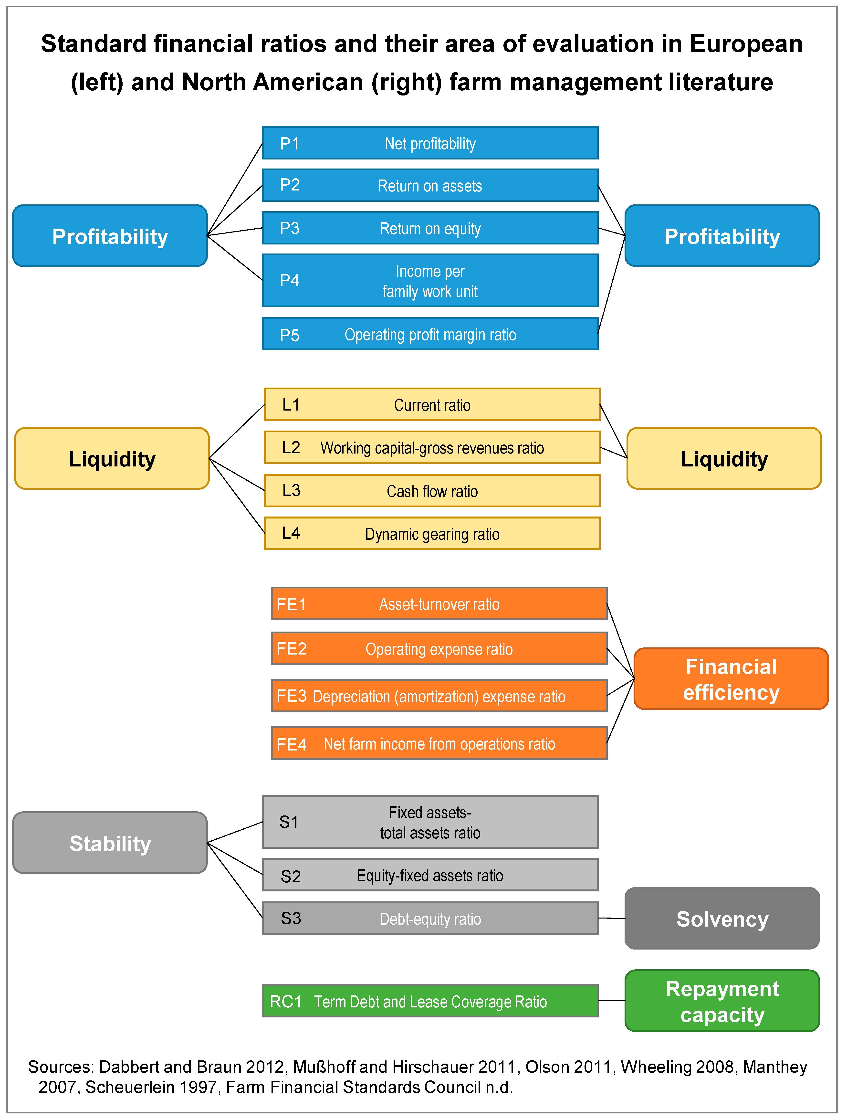
An article by Ahrendsen and Katchova [20] compared the financial ratios suggested by the American Farm Financial Standards Council [40] with those reported by the Agricultural Resource Management Survey (ARMS) [41]. A corresponding comparison does not exist for the pan-European FADN; whose ‘standard results’ do cover just a few high level financial ratios, such as farm net income and cash-flow, which apart from income per family work unit are all absolute figures [42]. We follow the recommendation from Ahrendsen and Katchova [20] and refer the ratios suggested by the Farm Financial Standards Council [40] rather than the shorter list of the ARMS [43]. From the review and selection process 17 ratios result. Figure 1 illustrates these ratios and their assignment to the different areas or indicators. This illustration shows similarities and differences across the Atlantic. Identical indicators, such as profitability and liquidity, partly are based on identical financial ratios, partly differ in practical implementation. Furthermore, we observe a partial congruence between stability and solvency. The indicators financial efficiency and repayment capacity or corresponding areas are not referred to in the European farm management textbooks. The formulas of all ratios are presented in the Appendix A.
3.1. Ratios for Profitability
Profitability ratios assess the ability of a farm to generate profit [27,39]. The ratios at hand relate the profit during a period to the factors of production such as capital (equity and total assets) and labour (unpaid family labour input) or the farm’s gross revenues. The higher the ratio, the better—this applies throughout the profitability ratios. Since different farm types use factors of production and other inputs in varying intensities, the farm type can affect these ratios.
Blanck and Bahrs [44] explained that net profitability is the best financial ratio, in order to have a proper standard of comparison and differentiation criterion for differently structured farms. Net profitability (P1) measures the relative factor income and it is calculated by dividing the farm net income (family farm income in case of a family farm) by the sum of opportunity cost that is, the imputed cost of equity (imputed capital cost are derived from the interest rate of Swiss government bond futures with a duration of 10 years) and the imputed cost for unpaid labour (opportunity cost of labour are derived from the averages of regional incomes in the 2nd and 3rd sector) [45]. In family farms, which are predominant in Europe [46] and particular in Switzerland, the farm family provides most of capital and labour. The family focuses on the remuneration of the ‘total complex of family-input’ [47]. Austrian and German farm accountancy analysis uses the business ratio net profitability [48,49].
In the following we look at the two components of the agricultural income, capital and labour remuneration, separately [39]. As a precondition, the other component needs to be valued by opportunity costs. In the first case the opportunity costs for family-own labour, that is, the imputed costs for unpaid labour, are deducted from the agricultural income. Relating the return to the total farm investment, yields the return on assets (ROA, P2). Return on equity (ROE, P3) refers to the farm net worth. Both ratios are frequently applied to measure profitability [26,50] and often used in sustainability assessments [7,45,51]. The ratio of ROE by ROA indicates the different effectivity of using debt capital versus equity capital [39].
In the case of the second component of the agricultural income, the remuneration of labour, the calculation is similar, while validating own capital (farm equity) by opportunity costs. The income per family work unit (FWU) (P4) is derived from the farm net income. Given current (low) interest rates [52], the remuneration of labour for Swiss farms outweighs the remuneration of own capital around 15 times [53]. The income per family work unit is an important criterion for agricultural policy and is a standard ratio of the Farm Accountancy Data Networks (FADN) [54,55]. Different sustainability approaches use this ratio to evaluate profitability [7,45,56,57].
Finally, the operating profit margin (P5) relates the profit to a farm’s gross revenue and hereby measures the operating efficiency [27,39,40]. US and also French farm accountancy data [58] comprise this ratio. Direct payments are considered as revenue due to their great importance in European agriculture [59], especially for Swiss farms. For example direct payments account in average for over 40% of gross revenue of Swiss farms in the mountain region in the years 2015 and 2016 [60]. We focus on sold agricultural products and direct payments but do not consider sales from agriculturally related activities (such as agri-tourism or machinery rental).
The return on assets respectively the return on assets are common ratios in European and North American farm management textbooks. Besides, European textbooks consider more keenly the remuneration of own, that is, family labour: P1 (net profitability) and P4 (income per family work unit) include this factor’s return.
3.2. Ratios for Liquidity
Liquidity describes a farm’s ability to meet its financial obligations. The current ratio (L1) is a common and very popular liquidity ratio [26]. It considers the farm’s ability to meet current debt obligations by current assets in the next twelve months [39]. Dividing current assets by current liabilities or short-term debt capital yields the current ratio (to avoid division by zero and subsequent missing values, we alter the denominator by adding one). This ratio is applied in different studies [50,61,62].
Working capital-gross revenues ratio (L2) relates the amount of working capital to business size measured by gross revenues. Generally, the higher the ratio working capital-gross revenues, the better a farm’s financial condition. However, interpretation of this ratio depends on farm type.
The cash flow ratio (L3) divides the cash flow by the turnover [63]. This ratio is used by banks [64] to compare farms within a farm type and it is also used for sustainability assessment [65]. The cash flow is the difference between receipts and payments of the farm. In our case turnover includes all sold products from agriculture and agriculture related activities as well as direct payments. The higher the cash flow ratio, the better the financial capacity [strength] [63] of a farm.
Dividing the farm liabilities including short and long-term debts by the cash flow, we obtain the dynamic gearing ratio, L4 [28]. This ratio, serves as liquidity ratio in different sustainability assessment tools [4,16,65]. It describes the necessary number of years to repay the farm liabilities by means of the cash flow.
Comparing the application of the four liquidity ratios, we see a common application in the North American and European hemisphere only for the current ratio. American farm management textbooks mention the working capital-gross revenues ratio whereas European financial analysis rather employ the cash flow ratio and the dynamic gearing ratio to assess farm’s liquidity.
3.3. Ratios for Financial Efficiency
Ratios on farms’ financial efficiency intend to measure how well financial resources were used to generate revenue [27,39]. Alone American textbooks discuss the category of financial efficiency and these measures of financial performance. All following ratios for financial efficiency are suggested by the Farm Financial Standards Council [40].
The asset-turnover ratio (FE1) assesses the efficiency in using capital [27,66] and is broadly applied [20,43,62]. To determine the asset-turnover ratio, the sum of farm production (farm turnover) plus direct payments is divided by (total) farm assets. The higher the asset-turnover ratio, the more efficient farm assets are used.
The operating expense ratio (FE2) indicates the share of operating expenses in farms’ gross revenue (in our case including direct payments). The higher the ratio, the greater the proportion of farm production that is required to cover operating expenses, that is, the less efficient a farm [67].
The depreciation expense ratio (FE3) indicates the share of depreciation in farms’ gross revenue. The lower the ratio, the less gross revenue is required to cover depreciation. Hence, the lower the depreciation expense ratio, the better. It is sensitive to farm type and the method of depreciation [40].
The interest expense ratio is another measure of financial efficiency [27,39,40]. This ratio indicates the share of farm interest expenses in the gross revenue. Swiss farms dispose of considerable shares of interest-free debts (so-called investment credits from public institutions for structural improvement). Such investments credits can lower the absolute interest expenses and hereby could influence this ratio. Therefore, this ratio is not considered. The lower the interest expense ratio, the better a farm’s financial efficiency.
3.4. Ratios for Stability and Solvency
European textbooks on agricultural accounting differentiate the areas liquidity and stability whereas American textbooks use the terms liquidity and solvency. They differentiate liquidity as a short-term measure—‘next 12 months’ [39]—whereas solvency considers all debts and takes the long-term perspective. Hereby, solvency indicate the viability of a farm after a financial adversity, that is, the ability to continue farm operations [40]. Alike, stability is regarded as viability of a farm [68] or the ability to retain profitability and liquidity. Hence, the terms stability and solvency are used in a similar context and therefore are illustrated together in this section.
For the fixed assets to total assets (S1), fixed assets (without livestock) are related to total assets [28,63]. This stability ratio shows the share of assets bound for a medium or long term, hereby analyses the asset structure and informs on the financial flexibility of a farm. Swiss FADN results report a similar ratio which includes livestock as fixed asset [60].
The equity to fixed assets ratio (S2) represents the relation of own capital or (farm) equity and the fixed assets [21]. This ratio is also called the golden rule for balance sheets, that is, to cover long-term assets by long-term credits or own capital [69]. The multiplication of S1 × S2 yields the farm debt-assets ratio, an international common ratio [28,43,70].
The farm debt to equity ratio (S3), third ratio which is relevant for both, stability and solvency, relates the debt or borrowed capital (liabilities) to the equity [26] and is suggested by the Farm Financial Standards Councils to report on a farm’s solvency [40]. It depicts how much the holders leveraged their equity in the business. The lower this ratio, the better since more equity is available to cover a farm’s debts.
3.5. Ratio for Repayment Capacity
North American farm financial analysis uses different measures of repayment capacity. This is the ability of a farm to meet cash flow obligations [39]. European textbooks do not cover a corresponding area of financial analysis; however, the topics liquidity and stability cover similar or corresponding issues. Three out of five common criteria to assess repayment capacity are absolute measures. The term debt coverage ratio (RC) is mentioned by textbooks [27,39] and commonly used in financial analysis [40,43]. This ratio assesses whether the farm generated enough cash to cover term debt payments [39]. Values greater than 1 or 100% indicate that debts are covered. The higher the ratio, the greater the margin to cover debt payments. This ratio’s value is low for farms without or with little debt; then, the denominator is zero (to avoid division by zero and subsequent missing values, we alter the denominator by adding one) or small and the resulting ratio is not computable or will be very high [40]. In the following analysis, the single ratio on repayment capacity due to its similar purpose is examined together with the ratios on stability/solvency, so that four areas of similar structure, each including at least four ratios and one, profitability, with five ratios.
4. Results
4.1. Descriptive Statistics
Table 1 presents the descriptive statistics of the pooled raw (untransformed) data on financial ratios. The statistics include the mean, the coefficient of variation and five percentiles (5th, 25th, 50th = median, 75th and 95th percentiles). The ratios for profitability indicate a generally low performance of Swiss dairy farms: for example, the majority of the farms (85.3% of observations for which P1 < 1) cannot remunerate the deployed capital and family labour at given opportunity cost. This means, they do not attain comparable incomes of other sectors. The ratio P3, return on equity, exhibits a high coefficient of variation. The large variation could be attributed to the calculation, in which the mostly low return is put in proportion to the typically voluminous equity. All profitability ratios reveal a generally low profitability of Swiss dairy farms.
The ratios on liquidity (apart from L3) exhibit extremely low and extremely high values; however, in the area between the first and the third quartile, the values lie in a common and non-critical range. Again, large coefficients of variation point to extreme values in the tails of the distribution.
Financial efficiency ratios range between zero and one (apart from singular extreme values). All ratios relate to gross revenue including direct payments. Ratios on stability and solvency inform on a farm’s capital structure. Extreme debt-to-equity ratios are below zero due to negative equity. Again, such unexpected values are mirrored in the highest coefficient of variation of all ratios. The other stability/solvency ratios are inconspicuous.
Finally, the term debt & lease coverage ratio (RC) covers a broad range of values and exhibits a considerable coefficient of variation. Strikingly, a considerable share of farms (close to 10%) do not rely on term debt or do not pay interest. For such farms, this ratio cannot be calculated.
4.2. Correlations between Financial Ratios
Table 2 reports the 136 Spearman’s rank correlations between the transformed, normalised and inverted (L4, FE2, FE3, S1 and S3 were inverted) financial ratios. Hence, a positive correlation means that the better one ratio, the better the other. Within the ratios, an almost uniform pattern of positive correlations can be observed (apart from the correlation FE1 × FE4, which is significantly negative). Three ratios—P1, FE2 and RC—feature positive correlations throughout (in case of P1, however, two correlations—those with L1 and L2—are not significant). Most ratios show few negative correlations. Only five ratios, P2, P5, FE1, L1 and S1 exhibit considerable shares of negative correlations. Only five negative correlations are below −0.1 with the highest correlation between L3 and FE1 with −0.38.
Within the five ratios on profitability, P1, net profitability, and P4, income per family work unit, stand out for few negative correlations and generally high synergies with other ratios. The synergies mainly appear within P, but also with regard to FE ratios (especially FE4, net farm income from operations ratio, which is relatively close to the profitability ratios).
Regarding the four ratios on financial efficiency, we observe two pairs of ratios. On the one hand, FE1 (asset-turnover ratio) and FE3 (depreciation expense ratio) seem similar according to their correlation coefficient and their coefficients with the other two FE ratios. On the other hand, FE2 (operating expense ratio) and FE4 (net farm income from operations ratio) exhibit a high correlation. This distinction is also reflected in a similar general structure of correlations with other ratios. The pair FE2 and FE4 shows considerably more synergetic relations and higher overall sums of correlation coefficients.
The ratios on liquidity exhibit relatively low synergies with other ratios, apart from L4, dynamic gearing ratio. Regarding L1 (current ratio) and L2 (working capital-gross revenues ratio), low synergies result from generally low correlations and especially from insignificant correlations between L1 and L2 with profitability ratios. Between L3, cash flow ratio, and FE1 as well as FE2 highest negative correlation coefficients show up, indicating trade-offs.
Finally, the ratios on stability, solvency as well as repayment capacity are examined together. These ratios exhibit a clear synergy with most other ratios apart from profitability. Negative correlations, although low, appear especially with P2 and P5. The S2 equity-fixed assets ratio and the S3 debt-equity ratio are highly correlated and feature similar results.
4.3. Correlations between Indicators
Table 3 presents the correlations between the four indicators (aggregated financial ratios), which are computed by weighing all transformed, normalised and partly inverted ratios equally. All of them are positive and significant but correlation is relatively weak (highest correlation coefficient is 0.42). Low correlation coefficients between financial efficiency and liquidity or between stability and profitability suggest that these indicators cover different issues. The aggregated indicator on financial efficiency shows the strongest correlation, both with profitability and stability.
4.4. Aggregate Performance Indicators
The aggregate performance indicator Y is composed by all 17 financial ratios. The average score is differentiated for four performance groups (quarter 1–4, Table 4). The mean score of Y ranges from 0.36 (first quarter, low performing farms) to 0.54 (fourth quarter, well performing farms). The following column shows the range between the first and fourth quarter of Y amounting to 0.18. Furthermore, Table 4 includes the mean values of the indicators and ratios across the quarters. All indicators and ratios exhibit monotonous increasing values across performance groups. This means that the fourth group of farms with the highest overall mean score has highest mean scores for all financial ratios. Looking at the range between boundary quarters (Q1–Q4), the ratios L1, L2, L4 and S3, all dealing with farm liabilities, show the lowest differences with ranges between the quarters below 0.10.
To construct the aggregate indicators ZE with one ratio from P, L and S as well as ZA with one ratio from P, L, FE and S/RC, correlation analysis between Y and all possible combinations of financial ratios were performed. Within the 36 combinations (4 P × 3 L × 3 S) of European aggregate indicators, the highest correlation with Y occurs with the combination P1/L1/S2, a correlation coefficient of 0.88; the correlation coefficient attains the combinations P1/L4/S1 and P1/L4/S2, as well as the corresponding triplets with P4. Within the aggregated indicators ZA, constructed from financial ratios referred by North American literature, the combination P5/L2/FE4/S3 exhibits the highest correlation with Y. The combination P5/L1/FE4/S3 nearly reaches that level.
Comparing the overall indicator Y (all 17 financial ratios) with the reduced sets ZE (P1/L1/S2) and ZA (P5/L2/FE4/S3) shows different levels of resulting performance indicators: the quarters of Y range between 0.36 and 0.54, ZE is on a remarkably lower level (quarters range from 0.18 to 0.39) whereas ZA lies slightly above Y (0.46 to 0.69). The difference between quarters of performance could be interpreted as an indicator’s ability to differentiate. The difference between quarters is higher for the reduced performance indicators ZA (0.23) and ZE (0.22) than for Y (0.18).
Considering the indicators profitability, liquidity, financial efficiency and stability/solvency-repayment capacity, we observe similar results across the quarters of the performance indicators. The scores are continuously increasing, providing a clear distinction between quarters. Continuously increasing scores can be detected also for the underlying financial ratios apart from FE1 in case of ZA: the average score of the quarter ZA4 exhibits the lowest value of all quarters.
Considering a larger range of values as ability to differentiate between farms, we observe highest differentiability with profitability (especially P1, P4, P5) followed by financial efficiency (especially FE2, FE4). The financial ratios on liquidity and stability/solvency-repayments capacity in contrast feature rather narrow ranges and accordingly low differentiability.
5. Discussion
The analysis of financial ratios in farm management textbooks revealed different approaches in North American and European textbooks. The areas profitability and liquidity are considered similarly and to a large part identical ratios are applied. American textbooks deal with financial efficiency and repayment capacity–areas of analysis not differentiated and explicated in European textbooks. Whereas the latter consider stability to analyse the financial structure. The areas stability (Europe) and solvency (America) partly overlap. These differences in farm management textbooks shed light on the challenge to introduce common, broadly employable standard financial ratios for economic sustainability assessment at the farm level.
5.1. Methodological Issues
Even though the present analysis is based on data from just one specific and specialised farm type and ratios as relative measures were considered, data problems occurred. Unexpected values, such as zero liabilities, any debt capital or interest rates of zero, resulted in missing values for ratio RC. The use of ratios led to very large numbers in case of division by very low values. This highlights the need for transforming the data range. Corresponding issues must be considered and anticipated, when selecting financial ratios for a sustainability assessment.
Financial statement information such as farm equity or farm debt typically are observed at a specific point in time, the reporting or accounting date. However, financial ratios should provide information on a period, usually a complete year. In this exploratory study, we did neglect this subtle distinction, due to the unbalanced nature of the panel data. In case of implementation, the recommendation of the Farm Financial Standards Council, to use the average values of the opening and the closing balance sheet [40] should be followed.
The analysis of financial ratios from farm accountancy data network (FADN) seems straightforward. However, such analysis is based on the willingness of farm operators to grant access [71]. In the Swiss FADN, farmers and accountants are paid for data provision. Important market players such as processors or supermarkets could draw on their market power to get access to such data from farms. However, providing farm financial data requires mutual trust.
Profitability ratios rely on imputed costs, for example, imputed labour (P1, P2, P3) and imputed capital costs (P1, P4, P5). The assumptions or legal requirements for labour cost imputation differ between countries: Swiss law refers to income in the second and third sector in the same region [72], whereas the Austrian [48] or the German [73] FADN approach rest upon agricultural wages. This reflects different normative assumptions on imputed labour costs that are reflected in the resulting ratios. When applying ratios that are sensitive to assumptions on imputed costs, this must be critically evaluated. This especially applies, if the farms are differently structured, for example, in case of examining simultaneously different farm types.
While we transform the outliers of the 1st and 99th percentile to the scores 0 and 1, Dolman et al. [74] determine the score 1 to the 10% best performing farms while the 10% worst performing ones were set to a value of 0. Looking at the descriptive statistics especially at the 5th and 95th percentiles (Table 1) a substantial loss of information would be the consequence. In case of L1, however, even after normalisation we have a highly right skewed distribution with few extreme values. This results in very low normalised ratios and a small range and differentiation (see Table 4).
The normalisation of the values to the range between 0 and 1 goes along with the assumption, that the higher a value, the better. This must not necessarily be the case. Hands-on literature on financial ratios often provides categories, that is, ranges together with a traffic light system [75]. This issue offers further research.
For the aggregated performance indicators, we used the simplest possible concept by weighting the indicators equally, which is motivated by analysing the basic relations of financial ratios. A logistic regression or a linear discriminant analysis, as suggested by Desbois [76], may represent more sophisticated approaches to building a score.
The present study is based on yearly data. Apart from L1 and L4, the mean values of financial ratios do not fluctuate considerably between years. Using perennial averages for the financial ratios would be an interesting alternative. This especially applies to L1, the current ratio, which is based on current farm assets and current liabilities. The use of two-year averages—as implemented in practical usage of ratios [20]—could alleviate heavy fluctuations while increasing demands on data availability. The variability of agricultural production and its’ effect on financial ratios argues also for the use of perennial averages. With less variation, the basis for the sustainability assessment would be more stable. However annual data offer two advantages: first, given an unbalanced panel, a standardisation to a uniform number of years that a farm has to be present in the sample would reduce the available data. Secondly, bearing in mind that a large investment (for example to build a new barn) affects financial ratios, with the use of yearly data the development of farms can be followed at different stages.
Farm types can differ considerably with regard to required assets or labour. Younger or beginning farmers exhibit higher debt-to-asset and asset turnover ratios [77]. Therefore, the evaluation of financial ratios for sustainability assessments should differentiate farm types and—if possible—should even be based on similar businesses [26]. The comparison of ratios is especially useful when similar farms with regard to structural and natural conditions of a specific farm type are compared. Weighing up a large number of benchmark farms with a higher degree of similarity within the benchmark group must be dealt carefully regarding the specific case and the impact on financial ratios.
5.2. Reduction of Financial Ratios
Within the financial ratios, positive correlations or synergies dominate. This is contrast to other findings with regard to the economic dimension [71]; though, the contrasting results are based on the rather qualitative SAFA method.
The mostly positive correlations between ratios and the observations that financial ratios continuously increase across quarters of the performance indicators Y, ZE and ZA suggest that a reduced set of indicators could be applied. Such a reduced set could simplify data acquisition and could increase the comprehensibility and acceptance of a sustainability assessment tool.
The most extreme case would be to focus on just one financial ratio. The correlation analysis (Table 2) points to financial ratios on profitability. These ratios provide a clear measure of economic performance. P1, net profitability, suggests itself as single financial ratio, since it exhibits positive correlation coefficients with all other financial ratios. The concentration on only one ratio which is highly dependent on assumptions on imputed costs, however, is also risky. Alternatively, the income per family work unit could be used.
6. Conclusions
Based on a literature review of financial ratios in farm management, 17 financial ratios were calculated for dairy farms from the Swiss FADN to assess their economic sustainability. The literature analysis revealed different usages of financial ratios across the North Atlantic Ocean and illuminated these differences regarding their application in farm management. Furthermore, the analysis considered these different cultures by differentiating a European and a North American accounting approach.
The harmonisation of financial ratios to scores allowed comparing and analysing them irrespective of challenges such as positive versus negative values, opposite direction of action, diverse magnitudes and differing units of measurement. Correlation analysis revealed synergies among financial ratios, most of them at a modest level. Accordingly, trade-offs are the exceptions between financial ratios. Also at the indicator level, we found small but positive correlations between profitability, liquidity, financial efficiency and stability/solvency/repayment capacity. We conclude that at least weak synergies exist between them. This result is also reflected by three performance indicators, Y compounding all ratios and ZE as well as ZA representing two subsets of ratios used in Europe (ZE) and North America (ZA). For all indicators, we observe that the overall performance is reflected by the scores of every financial ratio involved, which is in line with the predominant positive correlations between financial ratios.
This analysis represents a starting point for further elaboration and testing of a quantitative assessment of economic sustainability. The use and transformation of data offers further research opportunities with regard to the sensitivity of transforming and normalisation. Comparable studies of other Swiss farm types but also farms from other countries are necessary to assess whether the found positive correlations between financial ratios are specific for the farm type under consideration or whether it is a general agricultural phenomenon. In case of large datasets, the sample could be subdivided into group of similar farms (e.g., by farm size, farm turnover, regional origin, age of farm manager) to further refine validity of an assessment. We expect that such a procedure would reduce the observed heterogeneity. In addition, the question arises whether the found effects are transferable and the suggested approach is applicable to other industries to assess their economic sustainability.
Using financial ratios could also provide an impetus for farmers to consider the results of a sustainability assessment for farm management. For this purpose, the use and comparison of annual data instead of perennial means and the benchmarking with other, possibly similarly structured farms, would offer farm managers most benefit [26]. Finally, given the positive correlations a reduction of economic ratios within a sustainability assessment seems to be an option. This would reduce the necessary effort and may serve as an incentive to carry out an (economic) sustainability assessment more frequently.
Author Contributions
M.L. drafted the research idea and the research approach. M.E. and A.Z. reviewed the literature on farms’ economic sustainability assessments and farm management accounting to identify commonly applied financial ratios. M.E., I.B. and A.Z. performed data preparation and analysed the data. All authors are responsible for the original draft, reviewed the manuscript and discussed the results.
Acknowledgments
We thank Dierk Schmid for data extraction from the Swiss FADN database and three anonymous reviewers for their helpful comments. This study was conducted within Agroscope’s Work Programme 2014–2017.
Conflicts of Interest
The authors declare no conflict of interest.
Appendix A
Calculation of the ratios
Net profitability (P1)
Return on assets (P2)
Return on equity (P3)
Income per family work unit (FWU) (P4)
Operating profit margin ratio (P5)
Current ratio (L1)
Working capital-gross revenues ratio (L2)
Cash flow ratio (L3)
Dynamic gearing ratio (L4)
Asset turnover ratio (FE1)
Operating expense ratio (FE2)
Depreciation expense ratio (F3)
Net farm income from operations ratio (FE4)
Fixed assets-total assets ratio (S1)
Equity-fixed assets ratio (S2)
Debt-equity ratio (S3)
Term debt and lease coverage ratio (RC)
References
- Buckwell, A.; Nordang Uhre, A.; Williams, A.; Poláková, J.; Blum, W.E.H.; Schiefer, J.; Lair, G.J.; Heissenhuber, A.; Schieβl, P.; Krämer, C.; Haber, W. Sustainable Intensification of European Agriculture—A Review Sponsored by the RISE Foundation; RISE Rural Investment Support for Europe: Brussels, Belgium, 2014. [Google Scholar]
- Halog, A.; Manik, Y. Advancing integrated systems modelling framework for life cycle sustainability assessment. Sustainability 2011, 3, 469. [Google Scholar] [CrossRef]
- Cooper, T.; Hart, K.; Baldock, D. Provision of Public Goods through Agriculture in the European Union; Institute for European Environmental Policy: London, UK, 2009. [Google Scholar]
- Breitschuh, G.; Eckert, H.; Matthes, I.; Strümpfel, J.; Bachmann, G.; Breitschuh, T. Kriteriensystem Nachhaltige Landwirtschaft (KSNL). Available online: https://www.ktbl.de/fileadmin/produkte/leseprobe/11466excerpt.pdf (accessed on 9 August 2018).
- Schultheiß, U.; Zapf, R.; Döhler, H. Bewertung der Nachhaltigkeit landwirtschaftlicher Betriebe. LANDTECHNIK–Agric. Eng. 2008, 63, 293–295. [Google Scholar]
- Schader, C.; Grenz, J.; Meier, M.S.; Stolze, M. Scope and precision of sustainability assessment approaches to food systems. Ecol. Soc. 2014, 19, 42. [Google Scholar] [CrossRef]
- Meul, M.; Van Passel, S.; Nevens, F.; Dessein, J.; Rogge, E.; Mulier, A.; Van Hauwermeiren, A. MOTIFS: A monitoring tool for integrated farm sustainability. Agron. Sustain. Dev. 2008, 28, 321–332. [Google Scholar] [CrossRef]
- Food and Agricultural Organization of the United Nations (FAO). SAFA—Sustainability Assessment of Food and Agriculture Systems: Guidelines (Version 3.0); FAO: Rome, Italy, 2013. [Google Scholar]
- Christen, O. Nachhaltige Landwirtschaft—Ideengeschichte, Inhalte und Konsequenzen für Forschung, Lehre und Beratung. Ber. Landwirt. 1996, 74, 66–86. [Google Scholar]
- Landais, É. Agriculture durable: Les fondements d’un nouveau contrat social? Courrier de l’environnement de l’INRA 1998, 33, 5–22. [Google Scholar]
- Heißenhuber, A. Nachhaltige Landbewirtschaftung—Anforderungen und Kriterien aus Wirtschaftlicher Sicht; VDLUFA: Stuttgart, Germany, 2000; pp. 72–82. [Google Scholar]
- Slavickiene, A.; Savickiene, J. Comparative analysis of farm economic viability assessment methodologies. Eur. Sci. J. 2014, 10, 130–150. [Google Scholar]
- O’Donoghue, C.; Devisme, S.; Ryan, M.; Conneely, R.; Gillespie, P.; Vrolijk, H. Farm economic sustainability in the European Union: A pilot study. Stud. Agric. Econ. 2016, 118, 163–171. [Google Scholar] [CrossRef]
- de Olde, E.M.; Oudshoorn, F.W.; Sørensen, C.A.G.; Bokkers, E.A.M.; de Boer, I.J.M. Assessing sustainability at farm-level: Lessons learned from a comparison of tools in practice. Ecol. Indic. 2016, 66, 391–404. [Google Scholar] [CrossRef]
- Latruffe, L.; Diazabakana, A.; Bockstaller, C.; Desjeux, Y.; Finn, J.; Kelly, E.; Ryan, M.; Uthes, S. Measurement of sustainability in agriculture: A review of indicators. Stud. Agric. Econ. 2016, 118, 123–130. [Google Scholar] [CrossRef]
- Grenz, J. Response-Inducing Sustainability Evaluation (RISE); Bern University of Applied Sciences: Bern, Switzerland, 2017; p. 9. [Google Scholar]
- Lebacq, T.; Baret, P.V.; Stilmant, D. Sustainability indicators for livestock farming. A review. Agron. Sustain. Dev. 2013, 33, 311–327. [Google Scholar] [CrossRef]
- Diazabakana, A.; Latruffe, L.; Bockstaller, C.; Desjeux, Y.; Finn, J.; Kelly, E.; Ryan, M.; Uthes, S. A Review of Farm Level Indicators of Sustainability with a Focus on CAP and FADN; INRA: Rennes, France, 2014. [Google Scholar]
- Mishra, A.; Wilson, C.; Williams, R. Factors affecting financial performance of new and beginning farmers. Agric. Financ. Rev. 2009, 69, 160–179. [Google Scholar] [CrossRef]
- Ahrendsen, B.L.; Katchova, A.L. Financial ratio analysis using ARMS Data. Agric. Financ. Rev. 2012, 72, 262–272. [Google Scholar] [CrossRef]
- Zapf, R.; Schultheiß, U.; Doluschitz, R.; Oppermann, R.; Döhler, H. Nachhaltigkeitsbewertungssysteme—Allgemeine Anforderungen und vergleichende Beurteilung der Systeme RISE, KSNL und DLG-Zertifizierungssystem für nachhaltige Landwirtschaft. Ber. Landwirt. 2009, 87, 402–427. [Google Scholar]
- Dabbert, S.; Braun, J. Landwirtschaftliche Betriebslehre—Grundwissen Bachelor; Ulmer: Stuttgart, Germany, 2012; p. 288. [Google Scholar]
- Saltelli, A. Composite Indicators between Analysis and Advocacy. Soc. Indic. Res. 2007, 81, 65–77. [Google Scholar] [CrossRef]
- Organisation for Economic Co-operation and Development, Joint Research Centre of the European Commission. Handbook on Constructing Composite Indicators: Methodology and User Guide; OECD Publishing: Paris, France, 2008. [Google Scholar]
- Talukder, B.W.; Hipel, K.W.; vanLoon, G.W. Developing Composite Indicators for Agricultural Sustainability Assessment: Effect of Normalization and Aggregation Techniques. Resources 2017, 6, 66. [Google Scholar] [CrossRef]
- Barnard, F.; Akridge, J.; Dooley, F.; Foltz, J. Agribusiness Management; Routledge: New York, NY, USA, 2012. [Google Scholar]
- Wheeling, B.M. Introduction to Agricultural Accounting; Delmar Learning: Clifton Park, NY, USA, 2008; p. 329. [Google Scholar]
- Mußhoff, O.; Hirschauer, N. Modernes Agrarmanagement: Betriebswirtschaftliche Analyse- und Planungsverfahren; Vahlen: München, Germany, 2011. [Google Scholar]
- Basel Committee on Banking Supervision. Credit Ratings and Complementary Sources of Centre Quality Information; Basel Committee on Banking Supervision: Basel, Switzerland, 2000. [Google Scholar]
- Basel Committee on Banking Supervision. Studies on the Validation of Internal Rating Systems; Bank for International Settlements: Basel, Switzerland, 2005. [Google Scholar]
- Ohlson, J.A. Financial ratios and the probabilistic prediction of bankruptcy. J. Account. Res. 1980, 18, 109–131. [Google Scholar] [CrossRef]
- Cleary, S. The relationship between firm investment and financial status. J. Financ. 1999, 54, 673–692. [Google Scholar] [CrossRef]
- Delen, D.; Kuzey, C.; Uyar, A. Measuring firm performance using financial ratios: A decision tree approach. Expert Syst. Appl. 2013, 40, 3970–3983. [Google Scholar] [CrossRef]
- Hoop, D.; Schmid, D. Betriebstypologie ZA2015 (BT-ZA2015); Agroscope: Ettenhausen, Switzerland, 2016. [Google Scholar]
- Agroscope. Grundlagenbericht Zentrale Auswertung von Buchhaltungsdaten, Several Years (2003–2014). Available online: https://www.agroscope.admin.ch/agroscope/de/home/themen/wirtschaft-technik/betriebswirtschaft/za-bh/grundlagenbericht.html (accessed on 15 August 2018).
- Sachs, J.; Schmidt-Traub, G.; Kroll, C.; Durand-Delacre, D.; Teksoz, K. SDG Index and Dashboards Report 2017; Bertelsmann Stiftung and Sustainable Development Solutions Network (SDSN): New York, NY, USA, 2017. [Google Scholar]
- Müller-Benedict, V. Grundkurs Statistik in den Sozialwissenschaften: Eine Leicht Verständliche, Anwendungsorientierte Einführung in das Sozialwissenschaftlich Notwendige Statistische Wissen, 5th ed.; VS Verlag für Sozialwissenschaften: Wiesbaden, Germany, 2011. [Google Scholar]
- Jollands, N.; Lermit, J.; Patterson, M. The Usefulness of Aggregate Indicators in Policy Making and Evaluation: A Discussion with Application to Eco-Efficiency Indicators in New Zealand. 2003. Available online: https://openresearch-repository.anu.edu.au/handle/1885/41033 (accessed on 15 August 2018).
- Olson, K.D. Economics of Farm Management in a Global Setting; Wiley: Hoboken, NJ, USA, 2011. [Google Scholar]
- Farm Financial Standards Council. Financial Guidelines for Agriculture. Available online: https://www.ffsc.org/wp-content/uploads/2013/12/2014-Financial-Guidelines-for-Agriculture.pdf (accessed on 20 March 2018).
- National Research Council. Understanding American Agriculture: Challenges for the Agricultural Resource Management Survey; National Academies Press: Washington, DC, USA, 2008. [Google Scholar]
- European Commission. Farm Accountancy Data Network. Standard Results Indicator. Available online: http://ec.europa.eu/agriculture/rica/annex003_en.cfm#fi (accessed on 19 March 2018).
- USDA-ERS. ARMS Farm Financial and Crop Production Practices/Tailored Reports: Farm Structure and Finance; United States Department of Agriculture, Economic Research Service: Washington, DC, USA, 2018. Available online: https://www.ers.usda.gov/data-products/arms-farm-financial-and-crop-production-practices (accessed on 15 August 2018).
- Blanck, N.; Bahrs, E. Sind Erfolgreiche Betriebsleiter Tatsächlich Erfolgreich? Das Potenzial für Fehlinterpretationen bei der Kennzahl “Nettorentabilität”. Available online: http://www.gewisola.de/files/Schriften_der_GEWISOLA_Bd_46_2011.pdf (accessed on 15 August 2018).
- Breitschuh, G.; Eckert, H. Kriteriensystem nachhaltige Landwirtschaft; KTBL: Darmstadt, Germany, 2008. [Google Scholar]
- Eurostat. Agriculture Statistics—Family Farming in the EU. Available online: http://ec.europa.eu/eurostat/statistics-explained/index.php/Agriculture_statistics__family_farming_in_the_EU#Further_Eurostat_information (accessed on 6 October 2017).
- Poppe, K.J. Information Needs and Accounting in Agriculture; LEI: Den Haag, The Netherlands, 1991. [Google Scholar]
- LBG Österreich. Betriebswirtschaftliche Auswertung der Aufzeichnungen Freiwillig Buchführender Betriebe in Österreich 2016; LBG Österreich GmbH Wirtschaftsprüfung & Steuerberatung: Wien, Austria, 2017. [Google Scholar]
- Landesanstalt für Entwicklung der Landwirtschaft und der Ländlichen Räume. Landwirtschaftliche Betriebsverhältnisse und Buchführungsergebnisse: Wirtschaftsjahr 2016/17; LEL: Schwäbisch Gmünd, Germany, 2010. [Google Scholar]
- Argilés, J.M. Accounting information and the prediction of farm non-viability. Eur. Account. Rev. 2001, 10, 73–105. [Google Scholar] [CrossRef]
- Grenz, J.; Thalmann, C.; Stämpfli, A.; Studer, C.; Häni, F. RISE—A Method for Assessing the Sustainability of Agricultural Production at Farm Level. Available online: http://www.saiplatform.org/uploads/Library/RISEIndicatorsE_RDN1_2009.pdf (accessed on 15 August 2018).
- Swiss National Bank. Current Interest Rates. Available online: https://www.snb.ch/en/iabout/stat/statrep/id/current_interest_exchange_rates (accessed on 11 January 2018).
- Lips, M.; Gazzarin, C. Ex ante evaluation of the financial effects of investments. Agrarforschung Schweiz 2016, 7, 150–155. [Google Scholar]
- Hill, B. Farm Incomes, Wealth and Agricultural Policy: Filling the CAP’s Core Information Gap; CABI: Wallingford, UK; Cambridge, MA, USA, 2012. [Google Scholar]
- European Court of Auditors. Is the Commission’s System for Performance Measurement in Relation to Farmers’ Incomes Well Designed and Based on Sound Data? European Court of Auditors: Luxembourg, 2016; p. 74. [Google Scholar]
- Hennessy, T.; Buckley, C.; Dillon, E.; Donnellan, T.; Hanrahan, K.; Moran, B.; Ryan, M. Measuring Farm Level Sustainability with the Teagasc National Farm Survey; Teagasc: Athenry, Ireland, 2013; p. 27. [Google Scholar]
- Aggelopoulos, S.; Samathrakis, V.; Theocharopoulos, A. Modelling the Determinants of the Financial Viability of Farms. Res. J. Agric. Biol. Sci. 2007, 3, 896–901. [Google Scholar]
- Ministère de l’Agriculture et de l’Alimentation. Agreste—Chiffres et données—Agriculture. In Rica France—Tableaux Standard 2016; Ministère de l’Agriculture et de l’Alimentation: Paris, France, 2018. [Google Scholar]
- Manthey, R.P. Betriebswirtschaftliche Begriffe für die Landwirtschaftliche Buchführung und Beratung, 8th ed.; HLBS Verlag: Sankt Augustin, Germany, 2007; Volume 14, p. 99. [Google Scholar]
- Hoop, D.; Dux, D.; Jan, P.; Renner, S.; Schmid, D. Grundlagenbericht 2016. Stichprobe Einkommenssituation. In Zentrale Auswertung von Buchhaltungsdaten; Agroscope: Ettenhausen, Switzerland, 2017. [Google Scholar]
- Nasr, R.E.; Barry, P.J.; Ellinger, P.N. Financial structure and efficiency of grain farms. Agric. Financ. Rev. 1998, 58, 33–48. [Google Scholar]
- Purdy, B.M.; Langemeier, M.R.; Featherstone, A.M. Financial performance, risk, and specialization. J. Agric. Appl. Econ. 1997, 29, 149–161. [Google Scholar] [CrossRef]
- Wöhe, G.; Döring, U. Einführung in die Allgemeine Betriebswirtschaftslehre; Verlag Franz Vahlen: München, Germany, 2010. [Google Scholar]
- Hein, G. Wie Banken Bilanzen lesen. Agrarmanager 2015, 42–44. [Google Scholar]
- de Olde, E.M.; Oudshoorn, F.W.; Bokkers, E.A.M.; Stubsgaard, A.; Sørensen, C.A.G.; de Boer, I.J.M. Assessing the sustainability performance of organic farms in Denmark. Sustainability 2016, 8, 957. [Google Scholar] [CrossRef]
- Moss, C.B. Agricultural Finance; Taylor and Francis: London, UK, 2013; pp. 1–288. [Google Scholar]
- USDA–ERS. Documentation for the Farm Sector Financial Ratios. Available online: https://www.ers.usda.gov/data-products/farm-income-and-wealth-statistics/documentation-for-the-farm-sector-financial-ratios/ (accessed on 19 March 2018).
- Scheuerlein, A. Finanzmanagement für Landwirte: Beispiele, Anwendungen, Beurteilungen; BLV-Verl.-Ges.: München, Germany, 1997. [Google Scholar]
- Robinson, M. Measuring compliance with the golden rule. Fisc. Stud. 1998, 19, 447–462. [Google Scholar] [CrossRef]
- Department for Environment, Food and Rural Affairs. Balance Sheet Analysis and Farming Performance, England 2016/2017; Department for Environment, Food and Rural Affairs: London, UK, 2018.
- Schader, C.; Baumgart, L.; Landert, J.; Muller, A.; Ssebunya, B.; Blockeel, J.; Weisshaidinger, R.; Petrasek, R.; Mészáros, D.; Padel, S.; et al. Using the Sustainability Monitoring and Assessment Routine (SMART) for the Systematic Analysis of Trade-Offs and Synergies between Sustainability Dimensions and Themes at Farm Level. Sustainability 2016, 8, 274. [Google Scholar] [CrossRef]
- Schweizerischer Bundesrat. Verordnung über die Beurteilung der Nachhaltigkeit in der Landwirtschaft, SR 919.118, Bern, Switzerland. 1998. Available online: https://www.admin.ch/opc/de/classified-compilation/19983446/199901010000/919.118.pdf (accessed on 16 August 2018).
- BMEL. Die Wirtschaftliche Lage der Landwirtschaftlichen Betriebe. Buchführungsergebnisse der Testbetriebe des Wirtschaftsjahres 2016/2017; Bundesministerium für Ernährung und Landwirtschaft: Bonn, Germany, 2018. [Google Scholar]
- Dolman, M.A.; Vrolijk, H.C.J.; de Boer, I.J.M. Exploring variation in economic, environmental and societal performance among Dutch fattening pig farms. Livestock Sci. 2012, 149, 143–154. [Google Scholar] [CrossRef]
- Northwest Farm Credit Service. Understanding Financial Ratios and Benchmarks; Northwest Farm Credit Service: Spokane, WA, USA, 2016. [Google Scholar]
- Desbois, D. Introduction to scoring methods: Financial problems of farm holdings. Case Stud. Bus. Ind. Govern. Stat. 2014, 2, 56–77. [Google Scholar]
- Williamson, J.M. Following beginning farm income and wealth over time: A cohort analysis using ARMS. Agric. Financ. Rev. 2017, 77, 22–36. [Google Scholar] [CrossRef]
Figure 1.
Framework of quantitative economic sustainability indicators and underlying financial ratios for farm analysis.
Figure 1.
Framework of quantitative economic sustainability indicators and underlying financial ratios for farm analysis.


Table 1.
Descriptive statistics of the financial ratios.
| Ratio | Mean | Coefficient of Variation | Percentile | |||||
|---|---|---|---|---|---|---|---|---|
| 5% | 25% | 50% | 75% | 95% | ||||
| P1 | Net profitability | 0.63 | 0.66 | 0.09 | 0.38 | 0.59 | 0.83 | 1.30 |
| P2 | Return on assets | −0.05 | −1.77 | −0.21 | −0.08 | −0.03 | 0.00 | 0.05 |
| P3 | Return on equity | −9.60 | −23.96 | −56.84 | −17.36 | −7.21 | −0.92 | 9.74 |
| P4 | Income per family work unit (FWU) | 38,959 | 0.82 | 1148 | 21,267 | 35,560 | 52,942 | 89,989 |
| P5 | Operating profit margin ratio | −0.19 | −1.61 | −0.72 | −0.32 | −0.13 | 0.00 | 0.17 |
| L1 | Current ratio | 3977 | 7.43 | −16.83 | 2.28 | 8.58 | 27.33 | 32,399 |
| L2 | Working capital-gross revenues ratio | 0.30 | 2.41 | −0.67 | 0.11 | 0.30 | 0.52 | 1.24 |
| L3 | Cash flow ratio | 0.26 | 0.93 | 0.01 | 0.15 | 0.24 | 0.35 | 0.56 |
| L4 | Dynamic gearing ratio | 6.25 | 39.34 | −5.11 | 1.12 | 5.09 | 10.88 | 32.33 |
| FE1 | Asset-turnover ratio | 0.28 | 0.60 | 0.12 | 0.19 | 0.24 | 0.33 | 0.60 |
| FE2 | Operating expense ratio | 0.67 | 0.30 | 0.44 | 0.55 | 0.64 | 0.75 | 0.97 |
| FE3 | Depreciation expense ratio | 0.19 | 0.60 | 0.07 | 0.13 | 0.18 | 0.23 | 0.34 |
| FE4 | Net farm income from operations ratio | 0.32 | 0.55 | 0.06 | 0.22 | 0.32 | 0.42 | 0.58 |
| S1 | Fixed assets to total assets | 0.73 | 0.40 | 0.37 | 0.70 | 0.79 | 0.84 | 0.90 |
| S2 | Equity-fixed assets ratio | 0.84 | 3.65 | 0.12 | 0.47 | 0.71 | 1.02 | 1.89 |
| S3 | Debt-to-equity ratio | 0.85 | 49.12 | −0.26 | 0.14 | 0.59 | 1.38 | 4.57 |
| RC | Term debt & lease coverage ratio | 2809 | 5.15 | −10.58 | 1.39 | 5.18 | 13.55 | 25,786 |
Source: Swiss FADN data from the period 2003–2014 from 2404 dairy farms (unbalanced panel with N = 14,058 farm observations, for RC 13,975 observations).
Table 2.
Spearman’s rank correlations between transformed, normalised and-partly-inverted financial ratios. Negative correlations are highlighted by red font.
Table 2.
Spearman’s rank correlations between transformed, normalised and-partly-inverted financial ratios. Negative correlations are highlighted by red font.
| Financial Ratio | P1 ▫ | P2 ▫ | P3 ▫ | P4 ▫ | P5 ▫ | L1 ▫ | L2 ▫ | L3 ▫ | L4 ▫ | FE1 ▫ | FE2 ▫ | FE3 ▫ | FE4 ▫ | S1 ▫ | S2 ▫ | S3 ▫ | RC ▫ | ||||||||||||||||
|---|---|---|---|---|---|---|---|---|---|---|---|---|---|---|---|---|---|---|---|---|---|---|---|---|---|---|---|---|---|---|---|---|---|
| P2 ▫ | 0.87 | *** | 1 | ||||||||||||||||||||||||||||||
| P3 ▫ | 0.79 | *** | 0.84 | *** | 1 | ||||||||||||||||||||||||||||
| P4 ▫ | 0.99 | *** | 0.83 | *** | 0.75 | *** | 1 | ||||||||||||||||||||||||||
| P5 ▫ | 0.92 | *** | 0.95 | *** | 0.81 | *** | 0.90 | *** | 1 | ||||||||||||||||||||||||
| L1 ▫ | 0.01 | −0.02 | * | −0.01 | 0.01 | −0.03 | ** | 1 | |||||||||||||||||||||||||
| L2 ▫ | 0.01 | 0.01 | 0.02 | * | 0.00 | −0.04 | *** | 0.78 | *** | 1 | |||||||||||||||||||||||
| L3 ▫ | 0.28 | *** | 0.33 | *** | 0.34 | *** | 0.25 | *** | 0.25 | *** | 0.07 | *** | 0.17 | *** | 1 | ||||||||||||||||||
| L4 ▫ | 0.12 | *** | −0.01 | 0.20 | *** | 0.10 | *** | 0.02 | * | 0.08 | *** | 0.15 | *** | 0.32 | *** | 1 | |||||||||||||||||
| FE1 ▫ | 0.16 | *** | −0.11 | *** | −0.07 | *** | 0.20 | *** | 0.10 | *** | −0.08 | *** | −0.20 | *** | −0.38 | *** | 0.14 | *** | 1 | ||||||||||||||
| FE2 ▫ | 0.42 | *** | 0.26 | *** | 0.31 | *** | 0.39 | *** | 0.26 | *** | 0.11 | *** | 0.04 | *** | 0.30 | *** | 0.27 | *** | 0.04 | *** | 1 | ||||||||||||
| FE3 ▫ | 0.28 | *** | 0.05 | *** | 0.06 | *** | 0.31 | *** | 0.19 | *** | 0.00 | −0.05 | *** | −0.34 | *** | 0.09 | *** | 0.63 | *** | 0.04 | *** | 1 | |||||||||||
| FE4 ▫ | 0.62 | *** | 0.39 | *** | 0.42 | *** | 0.60 | *** | 0.39 | *** | 0.11 | *** | 0.13 | *** | 0.36 | *** | 0.24 | *** | −0.09 | *** | 0.60 | *** | 0.14 | *** | 1 | ||||||||
| S1 ▫ | 0.08 | *** | −0.15 | *** | −0.04 | *** | 0.10 | *** | −0.03 | ** | 0.17 | *** | 0.30 | *** | −0.07 | *** | 0.43 | *** | 0.57 | *** | 0.08 | *** | 0.43 | *** | 0.08 | *** | 1 | ||||||
| S2 ▫ | 0.05 | *** | −0.07 | *** | 0.16 | *** | 0.02 | * | −0.05 | *** | 0.10 | *** | 0.16 | *** | 0.17 | *** | 0.72 | *** | 0.09 | *** | 0.29 | *** | 0.07 | *** | 0.23 | *** | 0.43 | *** | 1 | ||||
| S3 ▫ | 0.02 | ** | −0.08 | *** | 0.29 | *** | 0.00 | −0.07 | *** | 0.08 | *** | 0.14 | *** | 0.19 | *** | 0.69 | *** | 0.04 | *** | 0.27 | *** | 0.05 | *** | 0.23 | *** | 0.36 | *** | 0.84 | *** | 1 | |||
| RC ▫ | 0.49 | *** | 0.37 | *** | 0.44 | *** | 0.47 | *** | 0.40 | *** | 0.06 | *** | 0.08 | *** | 0.39 | *** | 0.41 | *** | 0.09 | *** | 0.45 | *** | 0.03 | ** | 0.42 | *** | 0.16 | *** | 0.40 | *** | 0.36 | *** | 1 |
Source: Swiss FADN data from the period 2003–2014 from 2404 dairy farms (unbalanced panel with 14,058 farm observations). Statistical significance: ‘***’ for p < 0.001, ‘**’ for p < 0.01, ‘*’ for p < 0.05, ▫ transformed, normalised and-partly-inverted financial ratios.
Table 3.
Spearman’s rank correlations between indicators (aggregated financial ratios).
| Indicator | Profitability | Liquidity | Financial Efficiency | Stability/Solvency/Repayment Capacity | |||
|---|---|---|---|---|---|---|---|
| Liquidity | 0.19 | *** | 1 | ||||
| Financial efficiency | 0.42 | *** | 0.04 | *** | 1 | ||
| Stability/Solvency/Repayment capacity | 0.02 | * | 0.25 | *** | 0.40 | *** | 1 |
Source: Swiss FADN data from the period 2003–2014 from 2404 dairy farms (unbalanced panel with 14,058 farm observations). Statistical significance: ‘***’ for p < 0.001, ‘*’ for p < 0.05.
Table 4.
Aggregate performance indicators Y, ZE and ZA: average scores of performance groups (quarters–grouped according to mean overall score) and underlying indicators as well as financial ratios.
Table 4.
Aggregate performance indicators Y, ZE and ZA: average scores of performance groups (quarters–grouped according to mean overall score) and underlying indicators as well as financial ratios.
| Quarter Y1 | Quarter Y2 | Quarter Y3 | Quarter Y4 | Range Q Y1–Q Y4 | Quarter ZE1 | Quarter ZE2 | Quarter ZE3 | Quarter ZE4 | Range Q ZE1-Q ZE4 | Quarter ZA1 | Quarter ZA2 | Quarter ZA3 | Quarter ZA4 | Range Q ZA1–Q ZA4 | |
|---|---|---|---|---|---|---|---|---|---|---|---|---|---|---|---|
| Y | 0.36 | 0.43 | 0.47 | 0.54 | 0.18 | 0.37 | 0.43 | 0.47 | 0.53 | 0.16 | 0.37 | 0.44 | 0.47 | 0.53 | 0.15 |
| ZE | 0.19 | 0.24 | 0.28 | 0.37 | 0.19 | 0.18 | 0.24 | 0.28 | 0.39 | 0.22 | 0.20 | 0.25 | 0.29 | 0.35 | 0.15 |
| ZA | 0.48 | 0.57 | 0.61 | 0.67 | 0.20 | 0.49 | 0.57 | 0.62 | 0.66 | 0.17 | 0.46 | 0.56 | 0.61 | 0.69 | >0.23 |
| P | 0.41 | 0.53 | 0.60 | 0.69 | 0.29 | 0.41 | 0.53 | 0.60 | 0.69 | 0.27 | 0.40 | 0.53 | 0.61 | 0.69 | 0.29 |
| L | 0.37 | 0.40 | 0.42 | 0.46 | 0.09 | 0.38 | 0.40 | 0.42 | 0.46 | 0.08 | 0.38 | 0.40 | 0.42 | 0.47 | 0.09 |
| FE | 0.39 | 0.49 | 0.54 | 0.61 | 0.22 | 0.41 | 0.50 | 0.54 | 0.59 | 0.18 | 0.42 | 0.50 | 0.54 | 0.58 | 0.16 |
| S/RC | 0.28 | 0.30 | 0.32 | 0.41 | 0.13 | 0.28 | 0.30 | 0.33 | 0.40 | 0.11 | 0.29 | 0.32 | 0.33 | 0.37 | 0.07 |
| P1 ▫ | 0.23 | 0.37 | 0.47 | 0.61 | 0.38 | 0.23 | 0.37 | 0.47 | 0.61 | 0.37 | 0.23 | 0.37 | 0.48 | 0.59 | 0.36 |
| P2 ▫ | 0.57 | 0.67 | 0.73 | 0.80 | 0.23 | 0.57 | 0.67 | 0.74 | 0.79 | 0.22 | 0.54 | 0.67 | 0.75 | 0.82 | 0.28 |
| P3 ▫ | 0.54 | 0.61 | 0.64 | 0.67 | 0.13 | 0.54 | 0.61 | 0.64 | 0.66 | 0.12 | 0.52 | 0.62 | 0.65 | 0.67 | 0.15 |
| P4 ▫ | 0.24 | 0.36 | 0.45 | 0.59 | 0.36 | 0.24 | 0.36 | 0.45 | 0.59 | 0.35 | 0.24 | 0.37 | 0.46 | 0.58 | 0.33 |
| P5 ▫ | 0.47 | 0.62 | 0.71 | 0.80 | 0.33 | 0.47 | 0.62 | 0.72 | 0.79 | 0.31 | 0.45 | 0.63 | 0.71 | 0.80 | 0.34 |
| L1 ▫ | 0.11 | 0.12 | 0.13 | 0.16 | 0.05 | 0.10 | 0.10 | 0.11 | 0.21 | 0.11 | 0.12 | 0.13 | 0.13 | 0.15 | 0.03 |
| L2 ▫ | 0.50 | 0.51 | 0.52 | 0.56 | 0.06 | 0.51 | 0.52 | 0.52 | 0.55 | 0.04 | 0.47 | 0.50 | 0.52 | 0.60 | 0.13 |
| L3 ▫ | 0.32 | 0.38 | 0.43 | 0.48 | 0.16 | 0.34 | 0.39 | 0.43 | 0.46 | 0.12 | 0.34 | 0.37 | 0.41 | 0.50 | 0.16 |
| L4 ▫ | 0.56 | 0.60 | 0.62 | 0.64 | 0.07 | 0.58 | 0.60 | 0.62 | 0.63 | 0.05 | 0.59 | 0.60 | 0.61 | 0.63 | 0.04 |
| FE1 ▫ | 0.15 | 0.18 | 0.20 | 0.28 | 0.13 | 0.17 | 0.17 | 0.20 | 0.27 | 0.10 | 0.19 | 0.22 | 0.22 | 0.18 | −0.01 |
| FE2 ▫ | 0.54 | 0.67 | 0.72 | 0.78 | 0.24 | 0.56 | 0.68 | 0.73 | 0.75 | 0.19 | 0.57 | 0.66 | 0.72 | 0.76 | 0.20 |
| FE3 ▫ | 0.54 | 0.63 | 0.67 | 0.74 | 0.20 | 0.57 | 0.63 | 0.66 | 0.72 | 0.15 | 0.58 | 0.65 | 0.67 | 0.67 | 0.09 |
| FE4 ▫ | 0.33 | 0.48 | 0.56 | 0.65 | 0.32 | 0.33 | 0.50 | 0.57 | 0.61 | 0.28 | 0.33 | 0.46 | 0.54 | 0.69 | 0.36 |
| S1 ▫ | 0.14 | 0.17 | 0.20 | 0.34 | 0.20 | 0.17 | 0.17 | 0.20 | 0.31 | 0.14 | 0.19 | 0.20 | 0.20 | 0.26 | 0.07 |
| S2 ▫ | 0.21 | 0.24 | 0.26 | 0.35 | 0.14 | 0.19 | 0.24 | 0.27 | 0.36 | 0.16 | 0.23 | 0.26 | 0.27 | 0.31 | 0.07 |
| S3 ▫ | 0.61 | 0.66 | 0.67 | 0.69 | 0.07 | 0.63 | 0.66 | 0.67 | 0.68 | 0.05 | 0.61 | 0.66 | 0.67 | 0.69 | 0.08 |
| RC ▫ | 0.14 | 0.15 | 0.16 | 0.25 | 0.11 | 0.15 | 0.15 | 0.17 | 0.24 | 0.09 | 0.15 | 0.16 | 0.18 | 0.22 | 0.07 |
Source: Swiss FADN data from the period 2003–2014 from 2404 dairy farms. The score for each financial ratio ranges between 0 (poor result) and 1 (good result). ▫ transformed, normalised and-partly-inverted financial ratios.
© 2018 by the authors. Licensee MDPI, Basel, Switzerland. This article is an open access article distributed under the terms and conditions of the Creative Commons Attribution (CC BY) license (http://creativecommons.org/licenses/by/4.0/).
Share and Cite
MDPI and ACS Style
Zorn, A.; Esteves, M.; Baur, I.; Lips, M. Financial Ratios as Indicators of Economic Sustainability: A Quantitative Analysis for Swiss Dairy Farms. Sustainability 2018, 10, 2942. https://doi.org/10.3390/su10082942
AMA Style
Zorn A, Esteves M, Baur I, Lips M. Financial Ratios as Indicators of Economic Sustainability: A Quantitative Analysis for Swiss Dairy Farms. Sustainability. 2018; 10(8):2942. https://doi.org/10.3390/su10082942
Chicago/Turabian StyleZorn, Alexander, Michele Esteves, Ivo Baur, and Markus Lips. 2018. "Financial Ratios as Indicators of Economic Sustainability: A Quantitative Analysis for Swiss Dairy Farms" Sustainability 10, no. 8: 2942. https://doi.org/10.3390/su10082942
Note that from the first issue of 2016, this journal uses article numbers instead of page numbers. See further details here.