The Relationships between Supply Chain Capability and Shareholder Value Using Financial Performance Indicators

Abstract

The purpose of this paper is to explore which financial performance indicators (FPIs) evaluate the level of supply chain capability (SCC) that explicitly touches all of the business functions and processes within and beyond the company. The authors investigated nine FPIs that were selected from the financial statements of 155 companies within nine industries from 2011 to 2017 using Morningstar financial database and Gartner’s report. The authors find that suitable FPIs to measure SCC for shareholders’ value are return-on-assets (ROA), days-sales-outstanding (DSO), and current ratio (CR). This means that higher ROA, shortened DSO, and an appropriate level of CR could reach a sustainable supply chain. These results will help the industry to avert a major disruption in supply chain processes and activities using suitable financial performance indicators.

1. Introduction

Researchers in various fields have published numerous articles with diverse research designs that examine the financial impacts on supply chain capability (SCC). Supply chain management (SCM) has a significant impact on a company’s financial performance and stock price [1,2,3,4,5]. Supply chain management has a direct impact not only on financial indicators but also the marketing performance of an organization [6], such as increased market share and return on investments [7,8], lower total costs [9], improved customer relations [10], and increased operational efficiency, which includes higher-order fulfillment rates and shorter-order cycle times [9]. It also influences competitive advantage [6,11], and the supply chain strategy has a central position in creating shareholder value (SHV) [12] to assure sustainable supply chain [13].

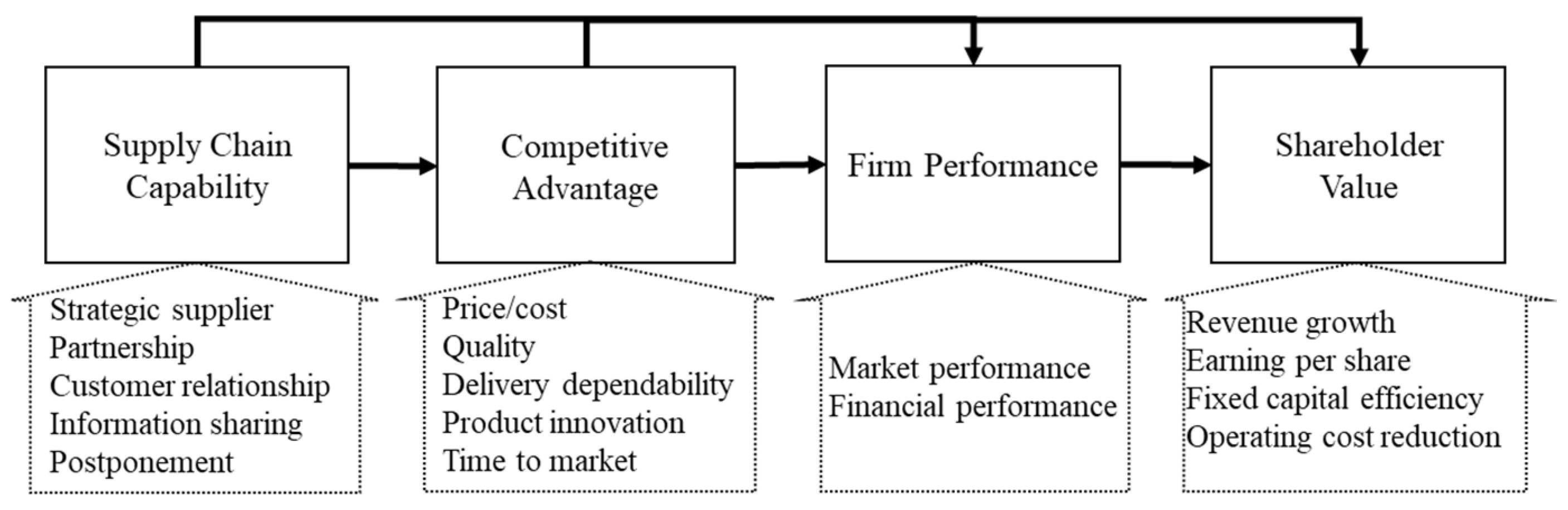
Supply chain management has been defined to explicitly recognize the strategic coordination between trading partners to improve an individual organization’s performance and to improve the whole supply chain [11,14]. Within leading companies, the SCC hinges on the health and well-being of the critical ecosystems within and around them, including people, the planet, and the partnerships formed to deliver customer solutions [15]. Higher supply chain capability has a positive effect on a firm’s performance regarding increased market share, shareholder value, revenue growth, fixed capital efficiency, operating cost reductions, and working capital efficiency [6,12] (see Figure 1). However, despite the increased attention paid to financial performance and SCM, relatively few studies utilize a wide range of financial indicators to cover company-wide financial performance ratios to evaluate supply chain capability. Many studies attempt to analyze working capital efficiency using cash-to-cash (C2C) cycle time, or one or two financial indicators, which limits access to company-wide supply chain processes and activities [6,16,17,18].

Supply chain management revolves around coordination, cooperation, and especially collaboration [4] among inter-organizational and business partners that are linked by the flow of materials, money, and information [19]. The complex relationships up and downstream make it difficult to acquire related data for the entire supply chain and SHV. To address this research gap, we provide a general framework to evaluate joint supply chain efforts to improve shareholder value using common SCC related financial performance indicators (FPIs) beyond C2C and categories of financial ratios to analyze company-wide health and try to find a competitive differentiator that influences shareholder value. The SCC is decisively important for operational efficiency, working capital management, and, ultimately, the bottom line, whereas a CEO ought to be fully engaged [11]. Therefore, the purpose of this research is to find the relationship between shareholder values and supply chain capability using companies’ financial statements from 2011 to 2017. The remainder of this paper is organized into five sections. Section 2 presents a review of the literature on conceptual frameworks with several hypotheses that address the characteristics of SCC regarding FPIs. Section 3 discusses the data collection process, research methodology, and results. Section 4 contains the discussion and implications, and Section 5 concludes.

2. Literature Review and Hypotheses

Economic value added (EVA) contributes to creating shareholder value [20] and gradually substitutes cost and profit objective functions to design a supply chain network [3,21]. Shareholders’ perspectives always inform managerial decisions because every company must do its best to keep shareholders and bondholders happy [22]. The ultimate purpose of the company is to maximize SHV for the long-term worth of the business to its owners [12]. The supply chain strategy has a central position in SHV creation and is the main source of competitive advantage [12]. The basic drivers to enhance SHV are revenue growth [12,15], operating cost reductions, fixed capital efficiency, working capital efficiency [12], earnings before interest, taxes, depreciation, and amortization (EBITDA), earnings per share (EPS) [12,22], and economic value added [20,23]. We have selected year-over-year changes in a firm’s revenue and EPS as our measures of shareholder value. These measures are often the first number that companies report to investors in their quarterly earnings call [12,15,22] because these measures provide evidence of value created by the firm to its shareholders.

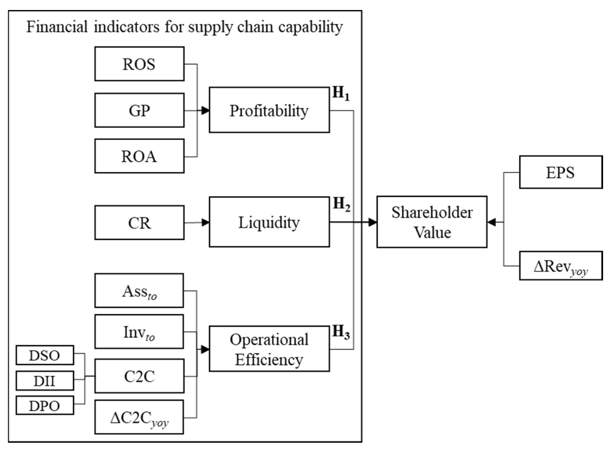
Financial metrics (or ratios) are a window into a company’s financial statements [22]. One important factor in business is an ongoing performance measurement [18]. However, previous literature has applied FPIs separately and not covered an extensive analysis of its supply chain capabilities and activities using comprehensive FPIs. We categorize the FPIs into three different areas that managers and other stakeholders in a business typically use to analyze the company’s SCC. Based on previous research, we classify 13 FPIs into three different groups [22]—profitability, operational efficiency and liquidity to measure SCC as well as SHV—as displayed in

Table 1. Financial Performance Indicators.

Category (1)	Financial Performance Indicators (FPIs)	Definitions	Influence on SC Capability (3)	Sources (2)
Profitability	Return-on-sales (ROS)	Net profit/revenues	Yes	[11,24,25,26,27,28,29,30]
	Gross profit margin (GP)	Gross profit/revenues	Yes
	Return-on-assets (ROA)	Net profit/assets	Yes
	Operating profit	Operating profit/revenue	NC	N/A
	Return on equity (ROE)	Net profit/shareholders’ equity	NC	N/A
Operational Efficiency	Days in inventory (DII)	Average inventory/(COGS/day)	Yes	[11,12,16,17,30,31,32]
	Inventory turnover	Cost of goods sold/Average inventory	Yes
	Days-sales-outstanding (DSO)	Ending accounts receivable/(revenue/day)	Yes
	Days payable outstanding (DPO)	Ending account payables/(revenue/day)	Yes
	Asset turnover	Sales/Average total assets	Yes
	C2C (cash-to-cash) cycle	DII+DSO-DPO	Yes
	C2C YoY	Percentage change of C2C year over year	Yes
	Property, plant, and equipment turnover (PPE)	Revenue/PPE	NC	N/A
Liquidity (Solvency)	Current ratio (CR)	Current assets/current liabilities	Yes	[29,33]
	Quick ratio (QR)	(Current asset-inventory)/current liability	NC
Leverage	Debt-to-equity	Total liabilities/shareholders’ equity	NC	N/A
	Interest coverage	Operating profit/annual interest charges	NC
Shareholders Value (SHV)	Revenue changes YoY (Year over Year)	% change of revenue to the same period of the previous year	Yes	[12,23]
	EPS (Earning per share) in dollars	(Net income - Dividends on preferred stock) / Average outstanding shares	Yes

⁽¹⁾ Based on [22]. ⁽²⁾ References just in case that FPIs have an influence on supply chain performance. ⁽³⁾ NC: No Commented on literature.

. We make four assumptions based on nine FPIs that have a positive relationship with supply chain performance.

Profitability ratios, such as net profit margin (ROS; return-on-sales), gross profit margin (GP), and return-on-assets (ROA) evaluate a company’s ability to generate profits through making sales and controlling expenses [22]. The ROS tells a company how much of every sale they keep after everything else has been paid for including people, vendors, lenders, the government, etcetera [22]. The ROS is net profit divided by revenue. The GP margin shows the basic profitability of the product or service and is calculated by gross profit divided by revenue. The GP indicates a potential problem for a company; when the GP is heading downward or becoming negative, it is assumed that the company has been considerably discounting products and is under severe price pressure [22]. The ROA shows how effectively the company uses its assets to generate profits; the equation is net profit over total assets. Most of the literature shows that SCM (green [34] and sustainable SCM [35] ) has a positive impact on a firm’s performance in areas like net profit margin [24,25,27], gross profit margin [12,30], and return-on-assets [11,15,26,28]. This discussion forms the basis of the following hypothesis with three indicators (ROS, GP, and ROA) together:

H1: 

Profitability (ROS, GP, and ROA) has a positive relationship with shareholder value.

Supply chain practices could improve cash flows and reduce the C2C cycle time [12,16,17,31,36], which would help free up cash and working capital to be invested in other products, better processes, and better financial performance [11,37]. Cash flow is a key indicator of a company’s financial health, along with profitability and shareholders’ equity [22,38]. The C2C covers the end-to-end of the supply chain and gives a certain diagnostic view based on inventory. Cash-to-cash is a critical performance measure of operational performance and has an impact on supply chain practices [12,16,17,36], but is not a one-size-fits-all strategy and managers in smaller firms should pay close attention to their C2C [38]. The C2C cycle time is defined as the sum of the day-sales-outstanding (DSO), plus the day-in-inventory (DII), minus the days payable outstanding (DPO), that is C2C = DSO + DII − DPO. The C2C is a critical performance measure and was also selected as the measure that has the greatest impact on supply chain practices because it shows the direct financial benefits of SCM [17,31] with improving the revenues of a company by 3% to 6% [16]. Wang’s [39] research results showed that reducing the C2C improved the operating performance of a firm. Prior research has found a significant negative relationship between profitability and the measures of working capital management, such as C2C [40,41].

Moreover, prior findings also indicate a significant negative correlation between C2C and measures of firm performance such as net sales and total assets [12,16,17,31,36]. It suggested that companies could increase profits by correctly managing the C2C cycle time and keeping the components of C2C at an optimum level. The C2C metric is an important measure because it bridges across inbound material activities with suppliers through manufacturing operations and outbound sales activities with customers [16]. The C2C increases the visibility of decision variables, increases the optimization of decisions in the supply chain, reduces sub-optimization of the financial decision within firms, and aids supplier decision-making by eliminating the uncertainty of customer actions [17]. The focus on managing C2C is the premise that a reduction in the cash conversion cycle time will lead to financial and operational improvements. However, within the supply chain, a leading player, likely located downstream, could take the initiative to shorten C2C significantly [42]. The strongest player in the supply chain could finance weak suppliers and customers [18]. This assumption could reduce the attractiveness of the product to the customers as the cost of goods increases. The operating cash flows are sensitive to declining sales and earnings [43]. From this alternate point of view, investors should focus on cash flows from mobilizing inventory (inventory turnover [15]), receiving investments, and using its assets efficiently to increase sales (asset turnover). Thus, operational efficiency encompasses not only C2C but also inventory turnover, asset turnover, and changes of the C2C year over year. With SCC, a firm should see increased operational efficiency in terms of increased asset and inventory turnover while reducing C2C and change of C2C year over year. Thus, we hypothesize:

H2: 

There is a negative relationship between SHV and operational efficiency (asset turnover, DSO, DII, DPO, and change of C2C year over year).

Liquidity ratios measure the short-term ability to pay debt obligations. They consist of the current ratio (CR) [33], the quick ratio, and the cash ratio. Liquidity ratios are closely connected to cash management in a supply chain [29,33]. Credit solvency is one of the essential pillars of financial status that can provide the necessary capital to a supply chain network [23]. Liquidity and solvency ratios measure the ability of the company to pay its obligations over the short and long runs. We focus more on short-run ability with CR. The current ratio measures a company’s current assets against its current liabilities. The current assets are those that can be converted into cash in less than a year; this figure (Figure 2) normally includes accounts receivables and inventory as well as cash [22]. Thus, we posit:

H3: 

There is a positive relationship between supply chain capability and liquidity (CR).

3. Research Methodology

We use the following procedure to develop our theory: (1) specify FPIs, (2) review literature on FPIs and supply chain capability, (3) collect data for FPIs and sample companies, (4) apply ordinary least square (OLS) regression analysis with all possible variables, (5) find an appropriate model assessing the variance inflation factor (VIF) for the severity of multicollinearity, normality, and homoscedastic test, (6) apply 1000 bootstrap replications if the tests are not significant statistically, and (7) verify the hypotheses using a significant level of dependent variables.

3.1. Data Collection

The Morningstar® Investment Research Center offers comprehensive financial data for investors, academics, and practitioners. First, we collected financial data from 311 companies within 18 industries based on 2015 data. Among the 311 companies, we chose 157 companies with more than $1 billion in revenue, and among the top 20 companies within each industry (see Appendix

Table A1. Industry, Top 25 Companies (Gr. 1) and Comparison Companies (Gr. 2).

#	Industry	Number	Top 25 Companies (Gr. 1)	Comparison Companies (Gr. 2)
1	Discount and retail store	18	Wal-Mart Stores, Inc., TESCO, Amazon.com, Nike, Home Depot	Costco Wholesale, Target, Dollar General, Dollar Tree, Dollarama, Lawson, Burlington Stores, Don Quijote Holdings, B&M European Value Retail, Distribuidora Internacional De, Pricesmart, Big Lots, Grupo Gigante SAB de CV
2	Restaurant	18	McDonald’s Starbucks	Compass Group, Yum Brands, Chipotle Mexican Grill, Restaurant Brands International, Yum China Holdings, Darden Restaurants, Aramark, Whitbread, Domino’s Pizza, Panera Bread, Minor International, Cracker Barrel Old Country Store, Jollibee Foods, Jack In The Box, The Wendy’s, Texas Roadhouse.
3	Household and personal products	18	Procter & Gamble (P&G), Unilever, L’Oreal, Colgate-Palmolive, Kimberly-Clark	Reckitt Benckiser, Henkel, The Estee Lauder, Kao, Newell Brands, Svenska Cellulosa, Beiersdorf, Clorox, Coty, Unicharm, Church & Dwight, Shiseido, Hengan International.
4	Apparel manufacturing	15	H&M, Inditex (1)	VF, Under Armour, Hanesbrands, Ralph Lauren, PVH, Michael Kors, Gildan Activewear, Carter’s Hugo Boss, Columbia Sportswear, UniFirst, Kate Spade, boohoo.com, Wacoal, G-III Apparel
5	Beverage and Foods	13	Coca-Cola, Pepsi Co., Diageo, Kraft Foods, Nestlé	Monster Beverage, Dr. Pepper Snapple Group, Arca Continental SAB de CV, Embotelladora Andina SA, ITO EN, Britvic, Cott, Refresco Group
6	Consumer Electronics, communication systems, software, data storage, and Electronics industry	27	Apple, Samsung Electronics, Hewlett Packard, Lenovo Group, Research In Motion, Nokia, Cisco Systems, Intel, Qualcomm, Schneider Electric, Microsoft, IBM, Seagate Technology, Dell (1)	Sony, Panasonic., Kyocera, Sharp, LG Display, Harman International Industrie, Electrolux, Alps Electric, Haier Electronics Group, Arcelik, Casio Computer, De’Longhi, Dometic Group, Skyworth Digital Holdings, GoPro
7	Pharmaceutical	19	Johnson & Johnson, GlaxoSmithKline	Pfizer, Novartis, Merck, Sanofi, AbbVie, Bristol-Myers Squibb, Bayer, Eli Lilly, AstraZeneca, Astellas Pharma, Otsuka Holdings, Chugai Pharmaceutical, Daiichi Sankyo, Ono Pharmaceutical, Kyowa Hakko Kirin, CSPC Pharmaceutical Group, Santen Pharmaceutical
8	Automotive	14	Toyota, Ford, BMW,	Daimler, Volkswagen, General Motors, Honda Motor., Nissan Motor., Tesla Motors., Audi, Renault, Hyundai Motor, Fiat Chrysler Automobiles, Suzuki Motor
9	Others	11	Cummins, Caterpillar, 3M, BASF	Compagnie de Saint-Gobain, LafargeHolcim, Tempur Sealy International, Fletcher Building, Ricoh, La-Z-Boy, Steelcase
		155	40 (2)	115

⁽¹⁾ Excluded from the analysis because of data acquisition limit in the Morning Star database.

). From 157 companies, 42 companies are the supply chain top-performers based on Gartner’s report from 2011 to 2017 [15]. Two companies, Dell and Inditex, were excluded because of limited data. We classified the selected 155 companies, which are 40 top-performers as a group (Gr. 1) and 115 companies as a group (Gr. 2) to compare the SCC. Among these 40 top-performing companies, 17 companies were chosen for seven consecutive years, one for six years, two for five years, two for four years, three for three years, five for two years, and ten companies for only one year. Both academics and practitioners refer to Gartner’s [44] Supply Chain Top 25 for SCC (Appendix Table A1). Most of the companies are located in North America (50%), especially the United States (45.8%), Europe (25%), and Asia (24%) including Japan (16%). Eighty companies (51.6%) are over $10 U.S. billion dollars, including 40 of Gartner’s top performers (

Table 2. Geographical Location and Annual Sales of Sample Companies.

Geographical Location					Total Company Annual Sales
					Annual Sales	#	%
North America	United States	71	78	50%	<1 billion U.S. Dollars	2	1%
	Canada	5			1–5 billion U.S. Dollars	51	33%
	Mexico	2			5–10 billion U.S. Dollars	22	14%
Europe	United Kingdom	12	38	25%	10–20 billion U.S. Dollars	24	15%
	Germany	10			20–30 billion U.S. Dollars	12	8%
	France, Sweden	4 each			30–40 billion U.S. Dollars	5	3%
	Switzerland	3			>40 billion U.S. Dollars	39	25%
	Netherlands	2
	Finland, Italy, Spain	1 each
Asia	Japan	25	37	24%
	China	5
	Korea	3
	Hong Kong, Philippines, Thailand, Turkey	1 each
South America	Chile	1		1%
Oceania	New Zealand	1		1%
Total		155		100%		155	100%

).

3.2. Analysis

In this section, the authors break down the two different parts. The first part focuses on the leading supply chain companies; the authors offer a leading companies’ ranking by applying data envelopment analysis (DEA) based on the ranking. The newly pooled ranking gives comprehensive information on which companies have supply chain capabilities. The second part applies OLS to find SCC related variables that have a relationship with SHV. For this analysis, we have two groups of companies: excellence SCC companies (Gr. 1) and non-excellence companies (Gr. 2).

Leading supply chain companies: The data envelopment analysis (DEA) can be used to measure efficiency using multiple input and output variables [45]. This research applies the DEA method to the preference voting method developed by Cook and Kress (CK) [46]. The CK model has been widely used as a decision measurement technique to balance the shortcomings of traditional techniques that are based on preference voting, in which the ranked voting data can be changed depending on the weight [47]. The authors applied the CK model to determine the excellence SCC companies based on the supply chain top 25 from 2011 to 2017, as determined by Gartner Incorporated [15,44]. Using Gartner’s ranking data for seven years, the authors tried to measure the comprehensive ranking by applying the preference voting method. (DEA CK is calculated using $Max Z_i=Max {\displaystyle \sum }_{j=1}^k{W}_j{V}_{ij}(\epsilon )$, where $Z_{i }$ is the long-term supply chain excellence for company i and $V_{ij}$ is the frequency of jth place rank of company i (i = 1, …, m, j = 1, …, k) subject to ${\displaystyle \sum }_{j=1}^k{W}_i{V}_{ij}\le 1{\forall }_i$, $W_j-W_{j+1}\ge d\left(j, \epsilon \right), {\forall }_j$, where $W_j$ is the coefficient of supply chain excellence and $W_k\ge d\left(k, \epsilon \right)$ for k = last ranking company. $d\left(·, \epsilon \right)$ is a discrimination intensity function with non-negative and non-decreasing $\epsilon$. The equation of $W_j-W_{j+1}\ge d\left(j, \epsilon \right)$ means that the weight value of $W_j$ of $V_j$ should be larger that the weight value $W_{j+1}$ of $V_{j+1}$. This paper applies $W_j\ge W_{j+1}+0.0050$ between the 1st to 10th rank, $W_j\ge W_{j+1}+0.0025$ between 11th to 25th, $W_j\ge W_{j+1}+0.0010$ between 26th to 35th, and $W_j\ge W_{j+1}+0.0005$ for 36th to 42nd (see Appendix

Table A2. Leading supply chain companies based on Gartner’s Top 25 companies from 2011 to 2017.

DEA CK Ranking	Company	SCC Index (1)	Difference of SCE	Gartner’s Supply Chain Ranking (2)
				# of Top 25	2017	2016	2015	2014	2013	2012	2011
1	Apple	1.0000		7	1 (3)	1 (3)	1 (3)	1	1	1	1
2	Amazon.com	0.9350	0.0650	7	3 (3)	3	1	3	3	2	5
3	McDonald’s	0.9300	0.0050	7	2	2	2	2	2	3	8
4	P&G	0.8650	0.0650	7	5 (3)	5 (3)	5 (3)	5	6	5	3
5	Unilever	0.8521	0.0129	7	1	1	3	4	4	10	15
6	Cisco Systems	0.8100	0.0421	7	4	7	6	7	7	8	6
7	Intel	0.7996	0.0104	7	6	4	4	8	5	7	16
8	Inditex	0.7901	0.0095	7	3	6	5	11	12	15	19
9	Coca-Cola	0.6862	0.1039	7	14	9	11	10	9	6	11
10	Samsung Electronics	0.6818	0.0044	7	25	8	8	6	8	13	10
11	Colgate-Palmolive	0.6680	0.0138	7	9	13	9	9	10	11	13
12	H&M	0.6041	0.0639	6	5	5	7	13	17	17
13	Wal-Mart Stores	0.5481	0.0560	7	18	16	13	14	13	9	7
14	Nike	0.4612	0.0869	7	8	11	10	12	14	14	20
15	PepsiCo	0.4355	0.0257	7	11	15	15	15	16	12	9
16	Starbucks	0.4310	0.0045	7	10	12	12	17	15	16	22
17	3M	0.3932	0.0378	7	12	14	14	18	19	21	24
18	Nestlé	0.3589	0.0343	7	7	10	17	25	21	18	18
19	Dell	0.3573	0.0016	3					11	4	2
20	Johnson & Johnson	0.3412	0.0161	7	13	21	21	22	25	22	21
21	HP	0.2933	0.0479	4	19	17				24	17
22	Kimberly-Clark	0.2724	0.0209	5	21	24	20	21		25
23	Cummins	0.2485	0.0239	4			23	24	23	23
24	Lenovo Group	0.2439	0.0046	5	24	25	18	16	20
25	Caterpillar	0.2109	0.0330	3				23	18	20
25	L’Oréal	0.2109	0.0000	3	20	19	22
27	Qualcomm	0.2081	0.0028	3			19	19	24
28	Research In Motion	0.2019	0.0062	2						19	4
29	Schneider Electric	0.1564	0.0455	2	17	18
30	BASF	0.1536	0.0028	2	16	20
30	Seagate Technology	0.1536	0.0000	2			16	20
32	BMW	0.1312	0.0224	2	22	22
33	Microsoft	0.0889	0.0423	1							12
34	IBM	0.0836	0.0053	1							14
35	Nokia	0.0809	0.0027	1	15
36	Ford Motors	0.0656	0.0153	1					22
37	GlaxoSmithKline	0.0628	0.0028	1		23
37	TESCO	0.0628	0.0000	1							23
37	Diageo	0.0628	0.0000	1	23
40	Toyota Motors	0.0600	0.0028	1			24
41	Home Depo	0.0572	0.0028	1			25
41	Kraft Foods	0.0572	0.0000	1							25

⁽¹⁾ SCC index based on DEA CK, which is a relative capability, not an absolute capability. ⁽²⁾ Data source: Gartner (2018-a). ⁽³⁾ Masters: If the companies place in the top 5 rankings for at least 7 out of the past 10 years (Source: https://www.gartner.com). When the companies are nominated as a Master, the ranking does not appear on the list. Therefore, the authors put the last ranking of the company.

), applying strong ordering [47,48]. The result gives two 42 × 42 matrices for each company’s ranking results ($W_j{V}_{ij})$ and a weight value of each company for each rank ($W_j$ for all of i). Based on the calculation, the authors reached the final ranking of SCC companies (the first column of Appendix Table A2 based on the third column). Based on this analysis, we divided Group 1 into two sub-groups; one group included those over 0.500 of DEA ranking ([Gr 1 *] top 13 among 42 excellence SCC companies with two excluded companies, such as Inditex and Dell, Appendix Table A2), and the other group included the remaining companies to apply analysis in the next section further. The Gr. 1 * companies were in the top 25 for seven years in a row and were in the top 10 for at least two years from 2011 to 2017 except H&M for 2011.

The relationship between SCC and SHV: We conducted OLS based on the previous section. We developed two models—the dynamic model (Equation (1)) and the pooled model (Equation (2))to see how the financial performance indicator-related supply chain capability has a relationship with the shareholder value for excellence SCC companies (Gr 1 * and Gr 1) and non-excellence companies (Gr 2). Equations (1) and (2) are composed of independent variables ([IVs] with selected FPIs related to SCC from previous research,$SH{V}_{it}$, for Gr. 1, and 2 or Gr. 1 *, 1, and 2. The C2C-related variables are average DSO, DII, DPO, average changes of C2C from 2011 to 2016 as IVs. We take the revenue changes and earning per share in dollars as DVs, $SH{V}_{it}$ for Equation (1) and $SH{V}_i$ for Equation (2).

The Dynamic Model with FPIs is $Y_{it}=\beta x_{\mathit{i}\mathit{t}-\mathbf{1}}+{\epsilon }_{it-1}$, where $x_{\mathit{i}\mathit{t}-\mathbf{1}}$ is the independent variable vector. This model assumes that all of the usual OLS assumptions have not been violated, and the effect of any given X and Y is constant across observations with no interaction in X. This model reflects carry-over activities in two consecutive years (see Figure 3) and gives a short-term perspective. This model takes into account the time change effect and does not focus exclusively on a separate period. To cope with the long-term point of view, the dynamic model incorporates carry-over activities into the model [49]. The idiosyncratic differences across years are of interest in dynamic or global changes in the supply chain.

$$\begin{array}{c}SH{V}_{it}={\beta }_0+{\beta }_1{\left(ROS\right)}_{it-1}+{\beta }_2{\left(GP\right)}_{it-1}+{\beta }_3{\left(ROA\right)}_{it-1}+{\beta }_4{\left(As{s}_{to}\right)}_{it-1}+{\beta }_{5}ln{\left(In{v}_{to}\right)}_{it-1}+\\ {\beta }_6{\left(\Delta C2C_{\_yoy}\right)}_{it-1}+{\beta }_7{\left(CR\right)}_{it-1}+{\beta }_{8}ln{\left(DSO\right)}_{it-1}+{\beta }_{9}ln{\left(DII\right)}_{it-1}+{\beta }_{10}ln{\left(DPO\right)}_{it-1}+{\epsilon }_{it-1}\end{array}$$

(1)

where i is companies, t is a year from 2012 to 2016 when i = 1,…m, t = 1,…,n. When we analyze two groups, Gr. 1 in the fourth column of Appendix Table A1, and Gr. 2 in the fifth column of Appendix Table A1. When we have three Groups, Gr. 1 includes excellence SCC companies below 0.5000 of DEA CK results in Appendix Table A2 (29 companies), and 1 * includes super excellence SCC companies that exceed 0.5001 (13 companies).

The pooled model with FPIs is $Y_i=\beta x_i+{\epsilon }_i$, where $x_i$ is the independent variable vector with the same assumption as a dynamic model. This single-period model, made by pooling the 5-year data on average (compound annual growth rate for the percentage data), enabled us to measure the relationship without the fluctuating performances of combined good and bad years and long-term horizons. Economic uncertainty refers to macroeconomic, financial, and market conditions that either partially or totally play a role in the supply chain. The supply chain foundation addresses the importance of relationships based on trust [4] and long-term orientation [50,51,52]. Instead of splitting raw data year over year, the pooled data (combined data) smooths out economic uncertainty and gives the long-term horizon. It may be more appropriate to generalize to a population by pooling data over time to test the long-term relationship and a wide range of collaboration. Pooled data increases the degree of freedom through a financial benefit of increased heterogeneity.

$$\begin{array}{c}SH{V}_i={\beta }_0+{\beta }_1{\left(ROS\right)}_i+{\beta }_2{\left(GP\right)}_i+{\beta }_3{\left(ROA\right)}_i+{\beta }_4{\left(As{s}_{to\_avg}\right)}_i+{\beta }_{5}ln{\left(In{v}_{to\_avg}\right)}_i+\\ {\beta }_6{\left(\Delta C2C\_yoy\_a\right)}_i+{\beta }_7{\left(CR\right)}_i+{\beta }_{8}ln{\left(DSO\right)}_i+{\beta }_{9}ln{\left(DII\right)}_i+{\beta }_{10}ln{\left(DPO\right)}_i+{\mathsf{\epsilon }}_i\end{array}$$

(2)

where i is companies when i = 1,…m. All of the IVs are average or geometric means (=${\left[{\displaystyle \prod }_{t=1}^n{\theta }_{it}\right]}^{1/n})$ for percentage data such as the ROS, GP, and ROA values from n = 2011 to 2015. To conduct OLS, we tested the models’ validity with the multicollinearity, normality and homoscedastic test using VIF, Doornik–Hansen omnibus (D-H) test, and Breusch–Pagan (B-P) test. The mean VIF of the dynamic and pooled models is 2.49 and 1.94 that is under 2.5 (see Table 5). A VIF detects the multicollinearity of IVs (predictors) in the regression analysis. The VIFs are usually calculated by [1/(1 − ${\mathrm{R}}_{\mathrm{i}}^2$)] with ith independent variables. In some studies, a VIF above 10 indicates a high correlation, and less than 10 is acceptable [53]. Five is the maximum level of VIF, and some conservatively use 2.5 [54]. We use 2.5 as the maximum level of VIF for analysis of the hypotheses. After conducting the VIF test, we get nine variables out of 11; two variables were removed including inventory turnover (Inv_to or Inv_{to_avg}), which is highly correlated with DII and C2C, which is highly correlated with DSO, DII, and DPO. The D-H and B-P tests show a rejection of the null hypothesis, which means the estimation of models are not normally distributed and homoscedastic of variance. Therefore, we conduct 1000 bootstrap replications to estimate $\widehat{{\theta }_i}$ where i = 1, 2, …., k (for this research k = 1000) from the observed value of $\widehat{\theta }$.

4. Discussion and Implications

Table 3. Group Statistics for Gr. 1 and Gr. 2 of Dynamic and Pooled Models.

Category	FPIs	Statistics for the Dynamic Model (Equation (1))				Statistics for the Pooled Model (Equation (2))
		Gr. 1, Mean (n = 92)	Gr. 2, Mean (n = 455)	Total, Mean (n = 547) (1)	Test of Equality (2)	Gr. 1, Mean (n = 33)	Gr. 2, Mean (n = 109)	Total, Mean (n = 142) (3)	Test of Equality (2)
Profitability	ROS	0.1273	0.0664	0.0766	0.000 ***	0.0941	0.0601	0.0680	0.058
	GP	0.4508	0.4100	0.4168	0.066	0.4906	0.4173	0.4343	0.084
	ROA	0.1169	0.0679	0.0761	0.000 ***	0.0875	0.0637	0.0692	0.072
Operational efficiency	$\Delta$C2Cyoy	−0.2615	−0.1961	−0.2071	0.883	−0.2064	-0.9396	−0.7692	0.460
	C2C	37.627	53.136	50.494	0.044 *	47.647	54.592	52.981	0.623
	DSO	37.925	46.231	44.594	0.012 *	44.061	43.703	43.786	0.957
	DII	58.644	80.229	76.908	0.001 ***	62.478	85.824	80.410	0.040*
	DPO	61.048	73.324	71.008	0.023 *	64.237	76.331	73.527	0.253
	Assto	0.0113	0.0111	0.0111	0.777	0.0506	0.0260	0.0317	0.338
	Invto	16.060	12.679	13.247	0.311	13.767	13.335	13.435	0.940
Liquidity	CR	1.6983	1.8390	1.8154	0.246	1.6467	1.8354	1.7916	0.339
SHV	$\Delta$Revyoy	0.0607	0.0847	0.0806	0.516	0.0172	0.0705	0.0581	0.036 *
	EPS	9.7322	3.4725	4.5253	0.001 ***	7.2913	3.3127	4.2373	0.189

⁽¹⁾ Total n = 766 with 219 missing data. ⁽²⁾ Test of equality of Group means (based on Wilk’s lambda statistics). ⁽³⁾ Total n = 155 with 13 missing data. *** Significant at α = 0.001; ** Significant at α = 0.01; * Significant at α = 0.05.

shows the descriptive statistics for Gr. 1 (excellence SCC companies), Gr. 2 (non-excellence SCE companies), and the total mean, and tests of equality between groups based on Wilk’s lambda for dynamic and pooled models.

Table 4. Group Statistics for the Dynamic and Pooled Model (Equation (1)) of Gr. 1 *, Gr. 1, and Gr. 2.

Category	FPIs	Statistics for the Dynamic Model (Equation (1))							Statistics for the Pooled Model (Equation (2))
		Gr. 1 *	Gr. 1	Gr. 2	Total	Gr. 1 * & 1	Gr. 1 & 2	Gr. 1 * & 2	Gr. 1 *	Gr. 1	Gr. 2	Total	Gr. 1 * & 1	Gr. 1 & 2	Gr. 1 * & 2
Profitability	ROS	0.1277	0.1174	0.0661	0.0748	-	0.0513 ***	0.0616 ***	0.1320	0.0849	0.0587	0.0686	-	-	0.0740 *
	GP	0.4791	0.4269	0.4098	0.4158	-	-	0.0692 *	0.4704	0.4690	0.4138	0.4279	-	-	-
	ROA	0.1241	0.1110	0.0689	0.0764	-	0.0421 ***	0.0552 ***	0.1246	0.0758	0.0651	0.0717	-	-
Operational efficiency	$\Delta$C2Cyoy ($\Delta$C2Cyoy_a)	−0.1809	−0.3482	−0.1954	−0.2082	-	-	-	−0.0303	−0.25932	−0.9505	−0.7637	-	-	-
	C2C	28.123	49.345	51.408	49.621	-	-	-	25.4033	59.935	48.479	49.906	-	-	-
	DSO	27.009	47.344	45.569	44.334	−20.335 **	-	−18.559 ***	25.5860	46.731	43.649	43.003	-	-	-
	DII	54.792	67.5067	80.921	78.037	-	-	−26.128 **	49.1057	74.218	82.280	78.539	-	-	-
	DPO	53.209	65.5043	73.301	71.278	-	-	−20.091 *	48.1620	71.202	74.428	72.043	-	-	-
	Assto	0.0119	0.0365	0.0319	0.0309	-	-	-	25.6946	7.9225	13.266	13.182	-	-	-
	Invto	13.889	9.3027	13.222	12.938	-	-	-	0.0116	0.1148	0.0120	0.0305	−0.103 ***	-	-
Liquidity	CR	1.5644	1.6919	1.8279	1.7976	-	-	-	1.5853	1.7114	1.8318	1.7910	-	-	-
SHV	$\Delta$Revyoy ($\Delta$Rev)	0.0760	0.0725	0.0764	0.0761	-	-	-	0.0561	0.0153	0.0773	0.0645	-	-	-
	EPS	14.235	4.1480	3.2979	4.1599	10.087 ***	-	10.937 ***	13.479	3.7396	3.1863	4.0831	-	-	-

*** Significant at α = 0.001; ** Significant at α = 0.01; * Significant at α = 0.05.

presents the information for Gr. 1 * (super excellence SCC; top 13 companies from Gr. 1 based on DEA CK in Section 3.1 and Section 3.2), Gr. 1, and Gr. 2 with the F-test (ANOVA), and post hoc test (Bonferroni) results. Based on the equality, F-, and Bonferroni tests, the dynamic model is more sensitive on a group-by-group basis than the pooled model, which means that the dynamic model shows more differences and reflects actual changes. The profitability is the order of Gr. 1 > Gr. 2, and Gr. 1 * > Gr. 1 > Gr. 2 in terms of ROS, GP, and ROA. However, ROS and ROA are only significant statistically. The efficiency of C2C related variables shows that the order of Gr. 1 < Gr. 2 is significant only for DII and Gr. 1 * < Gr. 2 < Gr. 1 for changes in C2C changes (ΔC2C_yoy), C2C, DSO, DII, DPO, and only DII is significant. Asset turnover and inventory turnover are the order of Gr. 1 > Gr. 2. Gr. 1 > Gr. 2 > Gr. 1 * for asset turnover, and Gr. 1 * > Gr. 2 > Gr. 1 for inventory turnover without significance. For SHV, the changes in revenue are not statistically significant group by group, regarding EPS Gr. 1 > Gr. 2 and Gr. 1 * > Gr. 1 > Gr. 2 with significance. As for liquidity, it is not significant statistically for the difference. The pooled model with three different groups is presented on the right-handed side in Table 4. For the pooled model for Equation (1) in Table 4, none of the FPIs are significant and are in nearly the same order with the dynamic model. The orders of each variable are the same as in Table 4. However, only two variables (ROA and asset turnover) from the category of profitability and operational efficiency are statistically significant. From the descriptive statistics (Table 3 and Table 4), we get significant information on SCC using FPIs. The excellence SCC companies are more profitable especially on ROS and ROA, operational efficiency with less C2C cycle time with shortening DSO and DII, and higher SHV with EPS.

Table 5. Results of the OLS and Bootstrap of the Dynamic and Pooled Models (Dependent variable is ∆Rev_yoy).

Category	FPIs	Dynamic Model		Pooled Model		Results
		OLS	Bootstrap (1000)	OLS	Bootstrap (1000)
		Coeff. (sig.) (1)		Coeff. (sig.) (1)
H1: Profitability	ROS	−0.4580 (0.106)	−0.4580 (0.212)	−0.9204 (0.041 *)	−0.9204 (0.061)	Supported partially
	GP	−0.0976 (0.349)	−0.0976 (0.401)	−0.1888 (0. 036 *)	−0.1888 (0.056)
	ROA	0.7201 (0.068)	0.7201 (0.052)	1.0044 (0.000 ***)	1.0044 (0.005 **)
H2: Operational efficiency	$\Delta$C2Cyoy	0.0071 (0.046 *)	0.0071 (0.502)	0.0002 (0.914)	0.0002 (0.964)	Supported weakly
	ln(DSO)	−0.0485 (0.009 **)	−0.0485 (0.064)	−0.0279 (0.014 *)	−0.0279 (0.011 *)
	ln(DII)	−0.0026 (0.898)	−0.0026 (0.871)	0.0261 (0.070)	0.0261 (0.166)
	ln(DPO)	0.0578 (0.056)	0.0578 (0.077)	0.0414 (0.038 *)	0.0414 (0.095)
	Assto	−1.5193 (0.658)	−1.5193 (0.619)	−0.2548 (0.003 **)	−0.2548 (0.680)
	ln(Invto)	-	-	-	-
H3: Liquidity	CR	0.0188 (0.220)	0.0188 (0.231)	0.0286 (0.015 *)	0.0286 (0.007 **)	Supported
Constant		0.02734	0.02734	−0.0908	−0.0908	-
Number of obs		544		137
Mean VIF		2.49	-	1.94	-
Doornik–Hansen test (sig.) H0: Normality		${\chi }^2$ = $24810$ $(0.000***$)	-	${\chi }^2$ = $8650$ $(0.000***$)	-
Breusch–Pagan test (sig.) H0: Homogenous		${\chi }^2$ = $12.63$ $(0.262$)	-	${\chi }^2$ = $28.01$ $(0.000***$)	-
F (or ${\chi }^2$)-value (sig.)		F-value = 2.26 (0.006 **)	${\chi }^2$ = $23.38$ $(0.0054**$)	F-value = 7.47 (0.000 ***)	${\chi }^2$ = $27.31$ $(0.001**$)
Adj R2		0.0205	0.0205	0.2998	0.2998

⁽¹⁾ Coefficients of OLS and bootstrap are the same but the significant levels are different. *** Significant at α = 0.001; ** Significant at α = 0.01; * Significant at α = 0.05.

shows the results of OLS and the 1000 bootstrap replications for the dynamic and pooled models using revenue changes as a DV that is an endogenous variable. We apply bootstrapping to avoid random data influence based on the D-H and B-P tests. For the analysis of the dynamic and pooled models, only the pooled model shows meaningful information. The dynamic model shows the actual changes and the pooled model shows the long-term-based result with SHV. Therefore, the DPO and CR have a high positive relationship, and ROS, ROA, DSO has a negative relationship with SHV for the pooled model.

Based on an analysis, ROS and GP have a negative relationship with SHV, and ROA has a positive relationship (support partially H1). Therefore, we find a positive relationship between profitability and SCC. The second hypothesis links operational efficiency, including C2C-related variables and asset and inventory turnover to SHV. Most previous research show that the C2C has negative relationships on SCC [6,12,16,17,18,31,37,39,55] and inventory periods [56]. However, our interesting research results show that the changes of C2C do not have any relationship to SHV; only DSO has a negative relationship when we have three categories of SCCs, as evidenced by the excellence SCC companies having a very short period of DSO. These results partially support the negative relationship between operational efficiency with the changes in revenue (SHV: ∆Rev_yoy) in the long-term horizon (H2). This research focuses more on liquidity using the current ratio for the ability of payment in the short run than solvency with long-run ability. It shows a positive relationship on SHV as previous research mentioned there was a relationship. Thus, H3 is supported. According to Reference [12], SCC creates SHV through the long-run worth of the business to its owners and investors.

Supply chain management is a complex, technology-driven discipline that reaches across functions, business processes, and corporate boundaries [2,4,11,20]. However, most research addresses the SCM problems in an isolated manner and focuses on data from a certain year without analyzing comprehensive financial performance indicators or only focuses on working capital-C2C. The top executives in a company tend to focus on financial performance measures, such as sales, profits, stock prices, and costs of capital to improve SCC [11], and on performance measures aligned with supply chain objectives across multiple firms [20]. Even though delivering SCM is important to financial outcomes, the previous research [18,57] focuses on short-term operative improvements due to complex networks of interrelated activities. The SCM has been the focus of growing research interest in improving profits for all parties involved in the integrated flow of products (or materials), information, and money across multiple companies. Therefore, our research has focused on a wide range of FPIs that influence supply chain capability and has taken into account short-term (dynamic model) and long-term (pooled model) points of view with the same period of data to improve the future financial performance of a particular firm and the supply chain as a whole.

The effectiveness of SCM is reducing DSO [11], C2C [41]; ensuring profitability, growth, and competitiveness [23]; and increasing in ROA [11]. However, shortening the C2C time cycle could also be achieved through delaying payment to suppliers and reducing accounts receivables from customers without any further effort on operational efficiencies, instead of eliminating days of inventory and frequent deliveries with small lot sizes. Shortening the payments to suppliers creates liquidity pressures for other companies in the supply chain. Within the supply chain, a leading player, likely located downstream, could take the initiative to shorten C2C significantly [42]. However, DII could be one of the best metrics to measure SCC instead of C2C [18]. The reduction of the inventory holding period has a positive effect on the C2C cycle time, both from an individual firm as well as a collaborative supply chain viewpoint. This implies that the supply chain parties should seek ways to reduce each member’s inventory holding period [56,58]. Such inventory reduction efforts can be realized using other alternatives such as operations technology, right batch sizes, just-in-time approaches, build-to-order production, vendor-managed inventory concepts [59], and enhanced end-to-end relationships through the sharing of information [12,51,56].

Supply chain capability is decisively important for operational efficiency, working capital management, and ultimately, the bottom line [11]. Operational efficiency has been central to some of the greatest success stories in recent business history, including Wal-Mart, Toyota, and Dell [55]. Operation efficiency can lead to high-revenue growth, lower inventory using cross-docking and responsive purchasing and distributing of goods, lower prices, and increased profits, but operational performance is difficult to realize [55]. To improve operational performance, a firm must use supply chain practices [6,37,55], change the business culture [55], and introduce six sigma [11] and lean techniques [60]. Specifying goals for improvements in these areas requires knowing where the company currently stands. Previous research shows that C2C could explain operational efficiency. Several studies proved that shortening C2C means reducing the terms of credit for the receiver and delaying payment to suppliers. However, if the company tries to reduce the C2C by shortening the DSO, it could reach the effectiveness of SCM in the long run for shareholders’ value.

Supply chain processes interface with multiple suppliers and customers and trigger collaborative activities in the long-term; these activities should be based on trust to minimize transaction costs [4,28,61]. A combined supplier-customer EVA analysis enables us to determine how collaborative action leads to the attainment of supply chain outcomes [20]. The pooled model is used to examine the interdependence of supply chain activities through the combined data of all FPIs within five years. This research shows that sustainable long-term finance outcomes could be possible through the positive relationship between customer and supplier, reducing operating expenses, and increasing profitability [20]. Shortening DSO gives way to the positive relationship in the long run between supplier and buyer, which is a source of competitive advantage and generates great returns.

5. Conclusions with Limitations and Future Research Directions

Among the financial indicators we used in this study to express supply chain capability, days-sales-outstanding (DSO) is one of the most important metrics to measure comprehensive supply chain capability in the category of operational efficiency, return-on-assets in profitability, and current ratio in liquidity in the long-term for shareholder value. In particular, super excellence SCC companies show very short DSO and DII. This means that supply chain benefits share not only themselves but also others by shortening payment times to reduce the financial pressure to suppliers. Relying on C2C to control supply chain management as shown on previous research [17,36,62], it possibly weakens their control supply chain capability and sustainability [13,63] beyond the company in the long-term, and makes it difficult to ensure that their suppliers are operating in a financially sustainable fashion [18]. From a sustainable supply chain perspective, if suppliers have weaker credit ratings and thus pay higher interest rates than their customers pay, collaborative supply chain finance could not be possible [64]. Supply chain management deals with several decision variables regarding warehousing dollars, transportation, and optimal inventory levels [11,23] as well as buy-or-make decisions, distribution centers, and other common measures used for global optimization instead of local optimization [18]. Many companies measure only what they can easily access [11] to see the factors that affect supply chain processes and activities. Supply chain management has become a complicated set of activities that involves many business functions and processes, along with competitive differentiators [11]. Financial performance is one of the essential pillars that provide the necessary capital to supply chain networks [23]. Therefore, we use a wide range of financial performance indicators to help measure the supply chain capability, ensuring that both customers’ expectations and stakeholders’ benefit. Other values of this research include a holistic approach to reach a collaborative supply chain to find supply chain capability along with financial sustainability.

There are several important areas for future research to measure the supply chain capability using financial performance indicators, such as extending it to the end-to-end supply chain network, buyer-supplier finance, the effect of the firm’s size and organizational/corporate culture, which have an important role to SCC and shareholders’ value.

References

- D’Avanzo, R.; Lewinski, H.V.; Wassenhove, L.V. The link between supply chain and financial performance. Supply Chain Manag. Rev. 2003, 7, 40–47. [Google Scholar]
- Ellram, L.M.; Liu, B. The financial impact of supply management. Supply Chain Manag. Rev. 2002, 6, 30–37. [Google Scholar]
- Hofmann, E.; Locker, A. Value-based performance measurement in supply chains: A case study from the packaging industry. Prod. Plan. Control. 2009, 20, 68–81. [Google Scholar] [CrossRef]
- Kwon, I.; Hong, S.-J.; Kim, S. Do collaborative relationships in supply chain pay-off? Int. J. Organ. Collect. Intell. 2017, 7, 45–55. [Google Scholar] [CrossRef] [Green Version]
- Singhal, V.R.; Hendricks, K.B. How supply chain glitches torpedo shareholder value. Supply Chain Manag. Rev. 2002, 6, 18–24. [Google Scholar]
- Li, S.; Ragu-Nathan, B.; Ragu-Nathan, T.S.; Subba Rao, S. The impact of supply chain management practices on competitive advantage and organizational performance. Omega 2006, 34, 107–124. [Google Scholar] [CrossRef]
- Prasad, S.; Tata, J. Information investment in supply chain management. Logist. Inf. Manag. 2000, 13, 33–38. [Google Scholar] [CrossRef]
- Shin, H.; Soenen, L. Efficiency of working capital and corporate profitability. J. Financ. Pract. Educ. 1998, 8, 37–45. [Google Scholar]
- Lin, F.; Huang, S.; Lin, S. Effects of information sharing on supply chain performance in electronic commerce. IEEE Trans. Eng. Manag. 2002, 49, 258–268. [Google Scholar]
- Tan, K.C.; Kannan, V.R.; Hanfield, R.B. Supply chain management: Supplier performance and firm performance. J. Purch. Mater. Manag. 1998, 34, 2–9. [Google Scholar]
- Slone, R.E.; Mentzer, J.T.; Dittmann, J.P. Are you the weakest link in your company’s supply chain? Harv. Bus. Rev. 2007, 85, 116–127. [Google Scholar]
- Christopher, M.; Ryals, L. Supply chain strategy: Its impact on shareholder value. Int. J. Logist. Manag. 1999, 10, 1–10. [Google Scholar] [CrossRef]
- Kot, S. Sustainable supply chain management in small and medium enterprises. Sustainability 2018, 10, 1143. [Google Scholar] [CrossRef] [Green Version]
- Feldmann, M.; Muller, S. An incentive scheme for true information providing in supply chains. Omega 2003, 31, 63–73. [Google Scholar] [CrossRef]
- Gartner. The Gartner Supply Chain Top 25. Available online: https://www.gartner.com/technology/supply-chain/top25.jsp (accessed on 11 April 2018).
- Farris, M.T., II; Hutchison, P.D. Cash-to-cash: The new supply chain management metric. Int. J. Phys. Distrib. Logist. Manag. 2002, 32, 288–298. [Google Scholar] [CrossRef]
- Farris, M.T., II; Hutchison, P.D.; Hasty, R.W. Using cash-to-cash to benchmark: Service industry performance. J. Appl. Bus. Res. (JABR) 2005, 21, 113–124. [Google Scholar] [CrossRef]
- Hong, S.-J. Is cash-to-cash cycle appropriate to measure supply chain performance? In Toward Sustainable Operations of Supply Chain and Logistics Systems; Kachitvichyanukul, V., Sethanan, K., Golinska-Dawson, P., Eds.; Springer: Berlin/Heidelberg, Germany, 2015. [Google Scholar]
- Gupta, S.; Dutta, K. Modeling of financial supply chain. Eur. J. Oper. Res. 2011, 211, 47–56. [Google Scholar] [CrossRef]
- Pohlen, T.L. A framework for evaluating supply chain performance. J. Transp. Manag. 2003, 14, 3. [Google Scholar]
- Klibi, W.; Martel, A.; Guitouni, A. The design of robust value-creating supply chain networks: A critical review. Eur. J. Oper. Res. 2010, 203, 283–293. [Google Scholar] [CrossRef]
- Berman, K.; Knight, J. Financial intelligence: A Manager’S Guide to Knowing What the Numbers Really Mean; Harvard Business Press: Boston, MA, USA, 2013. [Google Scholar]
- Longinidis, P.; Georgiadis, M.C. Managing the trade-offs between financial performance and credit solvency in the optimal design of supply chain networks under economic uncertainty. Comput. Chem. Eng. 2013, 48, 264–279. [Google Scholar] [CrossRef]
- Cao, M.; Zhang, Q. Supply chain collaboration: Impact on collaborative advantage and firm performance. J. Oper. Manag. 2011, 29, 163–180. [Google Scholar] [CrossRef]
- Chen, I.J.; Paulraj, A. Towards a theory of supply chain management: The constructs and measurements. J. Oper. Manag. 2004, 22, 119–150. [Google Scholar] [CrossRef]
- Craighead, C.W.; Hult, G.T.M.; Ketchen, D.J., Jr. The effects of innovation–cost strategy, knowledge, and action in the supply chain on firm performance. J. Oper. Manag. 2009, 27, 405–421. [Google Scholar] [CrossRef]
- Flynn, B.B.; Huo, B.; Zhao, X. The impact of supply chain integration on performance: A contingency and configuration approach. J. Oper. Manag. 2010, 28, 58–71. [Google Scholar] [CrossRef]
- Lanier, D., Jr.; Wempe, W.F.; Zacharia, Z.G. Concentrated supply chain membership and financial performance: Chain-and firm-level perspectives. J. Oper. Manag. 2010, 28, 1–16. [Google Scholar] [CrossRef]
- Longinidis, P.; Georgiadis, M.C. Integration of financial statement analysis in the optimal design of supply chain networks under demand uncertainty. Int. J. Prod. Econ. 2011, 129, 262–276. [Google Scholar] [CrossRef]
- Swink, M.L.; Golecha, R.; Richardson, T. Does supply chain excellence really pay off? Supply Chain Manag. Rev. 2010, 14, 14–21. [Google Scholar]
- Christopher, M.; Gattorna, J. Supply chain cost management and value-based pricing. Ind. Mark. Manag. 2005, 34, 115–121. [Google Scholar] [CrossRef] [Green Version]
- Ebben, J.J.; Johnson, A.C. Cash conversion cycle management in small firms relationships with liquidity, invested capital, and firm performance. J. Small Bus. Entrep. 2011, 24, 381–396. [Google Scholar] [CrossRef] [Green Version]
- Jin, S.H.; Jeong, S.J.; Kim, K.S. A linkage model of supply chain operation and financial performance for economic sustainability of firm. Sustainability 2017, 9, 139. [Google Scholar] [CrossRef] [Green Version]
- Kirchoff, J.F.; Tate, W.L.; Mollenkopf, D.A. The impact of strategic organizational orientations on green supply chain management and firm performance. Int. J. Phys. Distrib. Logist. Manag. 2016, 46, 269–292. [Google Scholar] [CrossRef]
- Ortas, E.M.; Moneva, J.; Álvarez, I. Sustainable supply chain and company performance: A global examination. Supply Chain Manag. Int. J. 2014, 19, 332–350. [Google Scholar] [CrossRef]
- Lee, H.J.; Song, S.H.; Hong, S.-J. Linking supply chain management and financial performances: Evidence from Korean companies. Korea Logist. Rev. 2010, 20, 119–143. [Google Scholar]
- Rice, J.B.; Hoppe, R.M. Supply chain vs. supply chain: The hype the reality. Supply Chain Manag. Rev. 2001, 5, 46–54. [Google Scholar]
- Guragai, B.; Hutchison, P.D.; Farris, M.T. Cash-to-cash (C2C) length: Insights on present and future profitability and liquidity. In Advances in Management Accounting; Burney, L.L., Malina, M.A., Eds.; Emerald Publishing Limited: Bentley, UK, 2019; pp. 133–151. [Google Scholar]
- Wang, Y.J. Liquidity management, operating performance, and corporate value: Evidence from Japan and Taiwan. J. Multinatl. Financ. Manag. 2002, 12, 159–169. [Google Scholar] [CrossRef]
- Lazaridis, I.; Tryfonidis, D. Relationship between working capital management and profitability of listed companies in the Athens stock exchange. J. Financ. Manag. Anal. 2006, 19, 931591. [Google Scholar]
- Raheman, A.; Nasr, M. Working capital management and profitability–Case of Pakistani firms. Int. Rev. Bus. Res. Pap. 2007, 3, 279–300. [Google Scholar]
- Losbichler, H.; Mahmoodi, F.; Rothboeck, M. Creating greater shareholder value from supply chain initiatives. Supply Chain Forum: Int. J. 2008, 9, 82–91. [Google Scholar] [CrossRef]
- Richards, V.D.; Laughlin, E.J. A cash conversion cycle approach to liquidity analysis. Financ. Manag. 1980, 9, 32–38. [Google Scholar] [CrossRef]
- Gartner. Gartner Supply Chain Top 25 Methodology. Available online: https://www.gartner.com/technology/supply-chain/top25.jsp (accessed on 19 April 2018).
- Coelli, T.; Rao, D.P.; Battese, G.E. An Introduction to Efficiency and Productivity Analysis; Kluwer Academic Publishers: Boston, MA, USA, 1998. [Google Scholar]
- Cook, W.D.; Kress, M. A data envelopment model for aggregating preference rankings. Manag. Sci. 1990, 36, 1302–1310. [Google Scholar] [CrossRef]
- Hong, S.-J.; Kim, T. Determining the priority of transport policies: With a special focus on the data, envelopment analysis using ranked voting data. Transp. Policy Stud. Rev. 2009, 12, 21–28. [Google Scholar]
- Noguchi, H.; Ogawa, M.; Ishii, H. The appropriate total ranking method using DEA for multiple categorized purposes. J. Comput. Appl. Math. 2002, 146, 155–166. [Google Scholar] [CrossRef] [Green Version]
- Tone, K.; Tsutsui, M. Dynamic DEA: A slacks-based measure approach. Omega 2010, 38, 145–156. [Google Scholar] [CrossRef] [Green Version]
- Zhang, C.; Hong, S.-J. Guanxi Culture: How it affects the business model of Chinese firms. In The China Business Model; Paulet, E., Rowley, C., Eds.; Elsevier: Amsterdam, The Netherlands, 2017. [Google Scholar]
- Zhang, C.; Hong, S.-J.; Ohana, M. Measuring guanxi in Sino-Franco buyer and supplier relationships. Glob. Bus. Organ. Excel. 2019, 38, 46–53. [Google Scholar] [CrossRef]
- Li, J.; Hong, S.-J. Towards a New Model of Supply Chain Risk Management: The Cross-Functional Process Mapping Approach. Int. J. Elect. Cust. Relatsh. Manag. 2007, 1, 91–107. [Google Scholar] [CrossRef]
- Hair, J.F., Jr.; Anderson, R.E.; Tatham, R.L.; Black, W.C. Multivariate Data Analysis, 7th ed.; Pearson: Noida, India, 2015. [Google Scholar]
- Allison, P. When Can You Safely Ignore Multicollinearity? Statistical Horizons. Available online: https://statisticalhorizons.com/multicollinearity (accessed on 16 May 2018).
- Hammer, M. Deep change: How operational innovation can transform your company. IEEE Eng. Manag. Rev. 2004, 32, 42. [Google Scholar] [CrossRef]
- Hofmann, E.; Kotzab, H. A supply chain-oriented approach of working capital management. J. Bus. Logist. 2010, 31, 305–330. [Google Scholar] [CrossRef]
- Gligor, D.M.; Esmark, C.L.; Holcomb, M.C. Performance outcomes of supply chain agility: When should you be agile? J. Oper. Manag. 2015, 33, 71–82. [Google Scholar] [CrossRef]
- Hong, S.-J.; Randall, W.; Han, K.; Malhan, A. Estimation viability of dedicated freighter aircraft of combination carriers: A data envelopment and principal component analysis. Int. J. Prod. Econ. 2018, 202, 12–20. [Google Scholar] [CrossRef]
- Pohlen, T.L.; Goldsby, T.J. VMI and SMI programs: How economic value added can help sell the change. Int. J. Phys. Distrib. Logist. Manag. 2003, 33, 565–581. [Google Scholar] [CrossRef]
- Martichenko, R.; Grabe, K. Building a Lean Fulfilment Stream: Rethinking Your Supply Chain and Logistics to Create Maximum Value at Minimum Total Cost; Lean Enterprise Institute: Cambridge, UK, 2010. [Google Scholar]
- Kwon, I.-W.; Hamilton, J.; Hong, S.-J. Trust and transaction cost in supply chain cost optimization: An exploratory study (Chapter 5 in Inter.-organizational Information Systems and Business Management: Theories and Researchers; Vaidya, K., Ed.; IGI Global Publishing: Pennsylvania, PA, USA, 2012. [Google Scholar]
- Randall, W.S.; Farris II, M.T. Supply chain financing: Using cash-to-cash variables to strengthen the supply chain. Int. J. Phys. Distrib. Logist. Manag. 2009, 39, 669–689. [Google Scholar] [CrossRef]
- Qu, Y.; Yu, Y.; Appolloni, A.; Li, M.; Liu, Y. Measuring Green Growth Efficiency for Chinese Manufacturing Industries. Sustainability 2017, 9, 637. [Google Scholar] [CrossRef] [Green Version]
- Wuttke, D.A.; Blome, C.; Heese, H.S.; Protopappa-Sieke, M. Supply chain finance: Optimal introduction and adoption decisions. Int. J. Prod. Econ. 2016, 178, 72–81. [Google Scholar] [CrossRef]
Figure 1.
Link supply chain capability and shareholder value. Source: [6,12] and authors’ elaboration.
Figure 2.
Research model: The relationship of supply chain capability and shareholder value. Source: Authors’ elaboration.
Figure 3.
Sharing resources between consecutive years and supply chain capability for the dynamic model (Equation (1)).