Macro Level Modeling of a Tubular Solid Oxide Fuel Cell

Abstract

This paper presents a macro-level model of a solid oxide fuel cell (SOFC) stack implemented in Aspen Plus^® for the simulation of SOFC system. The model is 0-dimensional and accepts hydrocarbon fuels such as reformed natural gas, with user inputs of current density, fuel and air composition, flow rates, temperature, pressure, and fuel utilization factor. The model outputs the composition of the exhaust, work produced, heat available for the fuel reformer, and electrochemical properties of SOFC for model validation. It was developed considering the activation, concentration, and ohmic losses to be the main over-potentials within the SOFC, and mathematical expressions for these were chosen based on available studies in the literature. The model also considered the water shift reaction of CO and the methane reforming reaction. The model results were validated using experimental data from Siemens Westinghouse. The results showed that the model could capture the operating pressure and temperature dependency of the SOFC performance successfully in an operating range of 1–15 atm for pressure and 900 °C–1,000 °C for temperature. Furthermore, a sensitivity analysis was performed to identify the model constants and input parameters that impacted the over-potentials.

1. Introduction

Fuel cells are devices that are capable of converting chemical energy from a fuel directly into electrical energy on a continuous basis, and due to this direct conversion they operate at higher efficiencies than conventional energy conversion devices. The types of fuel cells can be classified with respect to their operating temperatures and electrolyte compositions, which makes them suitable for different applications. Solid oxide fuel cells (SOFC) are especially suited for stationary power generation due to their sufficiently high operating temperatures (between 600 °C–1000 °C), which allow for integration with gas turbines or other bottoming cycles. The turbines and heat exchangers can utilize the heat released from the fuel cell which can reform the fuel internally. SOFCs can directly use natural gas, syngas from coal, and various biofuels. Furthermore, with the solid electrolyte, corrosion and electrolyte management problems are somewhat eliminated [1]. Additionally, due to their relatively low operating temperature compared to energy conversion devices which utilize combustion, the fuel based NO_X formation is negligible [2].

For the successful integration of SOFCs with other power generating technologies such as gas turbines, system simulation models that can accurately address optimization, heat management, fluctuating power demands and techno-economic evaluation are required. The first step towards developing these system models is to have a modular fuel cell model that can accurately predict the performance characteristics of a SOFC under varying operating and design conditions.

There are several different approaches presented in the literature for modeling the complex behavior of a SOFC: 0D models [3,4], 1D models [5], 2D models [6], quasi-2D models [7], 3D models [8], and combined 2D and 3D models [9]. The SOFC model presented in this study has been used to analyze various SOFC hybrid cycles. Therefore, a 0D model, which can be easily modified, has been developed. Possible future additions include heat transfer modeling and other considerations with respect to stack size. In the following sections, the model will be outlined, along with a sensitivity analysis of the input parameters. The model has been validated with experimental results from a Siemens Westinghouse tubular fuel cell.

2. SOFC Model Description

2.1. Methodology

A 0-dimensional, macro-level model was developed using fundamental equations of thermodynamics, chemical reactions, and electrochemistry. These equations rely on several input variables to specify the design parameters and operating conditions of the SOFC model. Experimental data from the literature had been used to validate the model, and a sensitivity analysis was carried out to investigate the effects of the model constants on the losses in the fuel cell. The general considerations and the assumptions in the model are:

• The fuel is a mixture of gases, which consists of any combination of CH₄, H₂, H₂O, CO, CO₂, O₂, and N₂.
• The air supplied to the fuel cell consists of any combination of O₂, N₂, CO₂, and H₂O.
• Chemical components behave as ideal gases at the operating temperature and pressure of the SOFC.
• Every SOFC within a stack operates at uniform temperature and pressure.

The SOFC model was written in FORTRAN 77, and executed from within Aspen Plus^®, a general process design and simulation software.

2.2. Chemical and Electrochemical Reactions

This study assumes three reactions are taking place within the SOFC; the CH₄-H₂O reforming reaction, the CO shift reaction, and the electrochemical oxidation of H₂. CO can be oxidized as well, but this reaction has been assumed to be negligible [4].

The electrochemical oxidation of H₂ takes place at the anode side according to Equation 1. This reaction requires oxygen ions, which are released by the reduction reaction of oxygen taking place at the cathode side of the SOFC. The latter reaction is shown in Equation 2. Combining the two half reactions, the overall electrochemical reaction can be obtained as shown in Equation 3.

$$H_2+O^{2-}\leftrightarrow H_{2}O+2e^{-}$$

(1)

$$\frac{1}{2}{O}_2+2e^{-}\leftrightarrow O^{2-}$$

(2)

$$H_2+\frac{1}{2}{O}_2\leftrightarrow H_{2}O$$

(3)

The CH₄-H₂O reforming and CO shift reaction take place at the anode side as well. As seen in Equations 4 and 5, H₂O is a reactant in both of these equations, thus as the electrochemical reaction takes place, the produced water will shift their equilibrium.

$$CO+H_{2}O\leftrightarrow C{O}_2+H_2$$

(4)

$$C{H}_4+H_{2}O\leftrightarrow CO+3H_2$$

(5)

The amount of H₂ reacted within the SOFC, and therefore the extent of the electrochemical reaction, is determined by the specification of an input parameter—the fuel utilization factor. It is defined as the ratio of moles of H₂ entering the fuel cell to the moles leaving:

$$U_f=\frac{\left[H_{2,in}\right]+\left[H_{2,out}\right]+\left[C{O}_{in}\right]-\left[C{O}_{out}\right]+3\left[C{H}_{4,in}\right]-3\left[C{H}_{4,out}\right]}{\left[H_{2,in}\right]+\left[C{O}_{in}\right]+4\left[C{H}_{4,in}\right]}$$

(6)

where the brackets denote molar flow rates. In order to find the anolyte exhaust composition, the reactions in Equations 4 and 5 are assumed to reach chemical equilibrium at the operating temperature of the fuel cell. Then, for both reactions, one can write:

$$k_{CO}=\frac{\left[C{O}_{2,out}\right]\left[H_{2,out}\right]}{\left[C{O}_{in}\right]\left[H_2{O}_{in}\right]}{\left(\frac{P/P_o}{N_T}\right)}^{\Delta \nu } \text{where} \Delta \mathsf{\nu }=0 (1+1–1–1)$$

(7)

and:

$$k_{C{H}_4}=\frac{\left[C{O}_{out}\right]{\left[H_{2,out}\right]}^3}{\left[C{H}_{4,in}\right]\left[H_2{O}_{in}\right]}{\left(\frac{P/P_o}{N_T}\right)}^{\Delta \upsilon } \text{where} \Delta \mathsf{\nu }=2 (3+1–1–1)$$

(8)

where k is the equilibrium constant at the operating temperature, N_T is the total number of moles and Δν is the difference between the stoichiometric coefficients of the products and the reactants from Equations 4 and 5.

Equations 6, 7, and 8 represent a system of non-linear equations and should be solved simultaneously for the outlet stream composition. The solution procedure can be simplified significantly if it is assumed that CH₄ is completely reformed within the SOFC, i.e., there is no CH₄ left in the exhaust [4,10]:

$$C{H}_{4,out}=0$$

(9)

Equations 6, 7, and 9 can now be solved, and the anolyte outlet composition can be found. The model also runs an internal control to verify that the air stream contains sufficient O₂ to react with the H₂. If the control fails, the fuel utilization factor is adjusted to a lower value.

2.3. Electrochemical and Thermodynamic Calculations

The model determines the operating point of the SOFC by performing several electrochemical calculations. The open-circuit voltage of the SOFC is first calculated. It is then discounted with the three overpotentials considered; the activation, ohmic, and the concentration losses. This gives the actual operating voltage of the SOFC, which is used to calculate the work output of the cell. To account for fuel crossover and internal current losses, an internal current density is added to the operating current density when calculating the overpotentials [3], i.e.,

$$i_{act}=i_{op}+i_I$$

(10)

where i_act is the actual current density (A/mol), i_op is the desired operating current density (A/mol), and i_I is the internal current density (A/mol).

The open-circuit voltage of a SOFC is usually very close to the reversible voltage given by the Nernst equation [11]. For the electrochemical reaction of H₂ the Nernst equation takes the following form:

$$V_{rev}=\frac{-\Delta g}{2F}+\frac{R_{u}T}{2F}\ln \left(\frac{\raisebox{1ex}{$P_{H_2}$}\!\left/ \!\raisebox{-1ex}{$P_{ref}$}\right.*{\left(\raisebox{1ex}{$P_{O_2}$}\!\left/ \!\raisebox{-1ex}{$P_{ref}$}\right.\right)}^{0.5}}{\raisebox{1ex}{$P_{H_{2}O}$}\!\left/ \!\raisebox{-1ex}{$P_{ref}$}\right.}\right)$$

(11)

where Δg is the Gibbs energy change (J/mol), F is the Faraday’s constant, R_u is the universal gas constant, T is the SOFC operating temperature (K), P_i is the partial pressures of the reactants and products, and P_ref is the reference pressure which is taken as 101,325 Pa.

Now, the overpotentials can be estimated using relations found in the literature. The activation loss can be evaluated using the Butler-Volmer equation [10]. It is assumed that each reaction is a one-step, single-electron transfer process such that the following form of the Butler-Volmer equation can be used [12]:

$$i_{act}=i_0\left(\exp \left(\beta \frac{F{V}_{activ}}{R_{u}T}\right)-\exp \left(-\left(1-\beta \right)\frac{F{V}_{activ}}{R_{u}T}\right)\right)$$

(12)

where i₀ is the exchange current density (A/mol), β is the transfer coefficient, and V_activ is the activation loss (V). This equation is applied to both the anode and the cathode, for which the exchange current densities can be found as follows [11,13]:

$$i_{0,anode}={\gamma }_{anode}+\left(\frac{P_{H_2}}{P_{ref}}\right)\left(\frac{P_{H_{2}O}}{P_{ref}}\right)\exp \left(\frac{E_{activ,anode}}{R_{u}T}\right)$$

(13)

$$i_{0,cathode}={\gamma }_{cathode}+{\left(\frac{P_{O_2}}{P_{ref}}\right)}^{0.25}\exp \left(\frac{E_{activ,cathode}}{R_{u}T}\right)$$

(14)

where γ is a pre-exponential factor (A/m²). Within the model, the exchange current densities are found, and then the activation loss for each electrode is found solving the Butler-Volmer equation. Since the Butler-Volmer equation is non-linear, the solution for the activation loss, V_activ, is determined numerically using the secant method.

The ohmic loss is due to resistance of electron flow in the electrodes and ion flow in the electrolyte. It can be determined using Ohm’s law [3,14]:

$$V_{Ohm}=i_{act}R$$

(15)

where i_act is the actual current density (A/m²), and R is the total ionic and electronic resistance (Ωm²). The total resistance can be estimated using the empirical correlation given in Equation 16 [14]:

$$R={\displaystyle \sum _i{A}_i\exp \left(\frac{B_i}{T}\right)}$$

(16)

where i refers to the cell component (anode, cathode, electrolyte, and interconnect), and A_i (Ω-m²) and B_i (K) are constants.

The concentration loss is found using the following relation [3,14,15]:

$$V_{conc}=-\frac{R_{u}T}{2F}\ln \left(1-\frac{i_{act}}{i_L}\right)$$

(17)

where i_L is the limiting current density (A/mol). The concentration loss within a SOFC is dependent on both molecular and Knudsen diffusion. The evaluation of the diffusion coefficients is outside the scope of this paper, but the effect of pressure on the concentration loss has been modeled using a pressure adjusted limiting current density as proposed by [14]:

$$i_{L,adj}=i_L{\left(\frac{P}{P_{ref}}\right)}^a$$

(18)

where P is the SOFC operating pressure, and a is a constant. Now, the operating voltage of the SOFC can be found:

$$V_{act}=V_{rev}-V_{activ}-V_{Ohm}-V_{conc}$$

(19)

The power output of the SOFC can be found from the operating voltage, actual current density, and the active cell area (Λ, m²):

$$\dot{W}=i_{act}\Lambda V_{act}$$

(20)

Once the outlet stream compositions and the power output of the SOFC are determined, 1st Law of Thermodynamics is applied to calculate the heat released by the SOFC:

$$\dot{Q}=\dot{m}\left(h_{in}-h_{out}\right)-\dot{W}$$

(21)

It should be noted that enthalpies of the inlet and outlet streams are calculated by the Aspen Plus^® engine.

3. Model Inputs and Outputs

The model is able to accept any fuel stream containing CH₄, H₂, H₂O, CO, and CO₂. The user can specify the fuel stream composition in terms of either mole or mass fractions and total mole flow, or mole or mass flow rates of individual components directly. The inlet temperature and pressure of the SOFC must also be specified. It should be noted that the pressure in the fuel cell is assumed to be constant throughout whereas the outlet stream temperature is calculated by adding a fraction of the isothermal enthalpy change on the outlet stream energy in order to take the commonly observed temperature rise in SOFCs into account.

To solve the above equations and determine the operating point of the SOFC, the model also requires several input parameters which are listed in Table 1 along with their values determined by the model validation process. These values are specified within the FORTRAN model, and can be easily modified by the user through the Aspen Plus^® interface.

Table 1. Model’s input parameters.

Parameter	Value	Units
Fuel utilization factor, Uf	0.85	-
Actual current density, iact	3200	A/m2
γanode (Equation 13)	2.0 × 108	A/m2
γcathode (Equation 14)	1.5 × 108	A/m2
Transfer coefficient (anode), βanode	0.5	-
Transfer coefficient (cathode), βcathode	0.5	-
Activation energy (anode), Eactiv,anode	105	kJ/mol
Activation energy (cathode), Eactiv,cathode	110	kJ/mol
Constant A (Equation 16)	2.0 × 108	Ω-m2
Constant B (Equation 16)	9000	K
Limiting current density, iL	6500	A/m2
Limiting current density correction factor a (Equation 18), a	0.05	-

Table 1. Model’s input parameters.

Parameter	Value	Units
Fuel utilization factor, Uf	0.85	-
Actual current density, iact	3200	A/m2
γanode (Equation 13)	2.0 × 108	A/m2
γcathode (Equation 14)	1.5 × 108	A/m2
Transfer coefficient (anode), βanode	0.5	-
Transfer coefficient (cathode), βcathode	0.5	-
Activation energy (anode), Eactiv,anode	105	kJ/mol
Activation energy (cathode), Eactiv,cathode	110	kJ/mol
Constant A (Equation 16)	2.0 × 108	Ω-m2
Constant B (Equation 16)	9000	K
Limiting current density, iL	6500	A/m2
Limiting current density correction factor a (Equation 18), a	0.05	-

Using these input parameters, the SOFC model is able to calculate the composition of the exhaust streams as well as the work and heat released. The model outputs several electrochemical properties of the SOFC listed in Table 2.

Table 2. Model’s output parameters.

Parameter	Units
Nernst voltage, Vrev	V
Actual operating voltage, Vact	V
Overall activation loss, Vactiv	V
Ohmic loss, VOhm	V
Exchange current density (anode), i0,anode	A/m2
Exchange current density (cathode), i0,cathode	A/m2
Activation loss (anode and cathode)	V
Pressure adjusted limiting current density, iL,adj	A/m2
Power produced, W	W
Heat produced, Q	W

Table 2. Model’s output parameters.

Parameter	Units
Nernst voltage, Vrev	V
Actual operating voltage, Vact	V
Overall activation loss, Vactiv	V
Ohmic loss, VOhm	V
Exchange current density (anode), i0,anode	A/m2
Exchange current density (cathode), i0,cathode	A/m2
Activation loss (anode and cathode)	V
Pressure adjusted limiting current density, iL,adj	A/m2
Power produced, W	W
Heat produced, Q	W

4. Results and Discussion

A sensitivity analysis was carried out to investigate the influence of the model constants and parameters on the SOFC loss calculations. Then, the model was compared to experimental results from Siemens Westinghouse as presented in [1]. When performing the sensitivity analysis, the values given in Table 1 were used, varying only the parameters studied for each run.

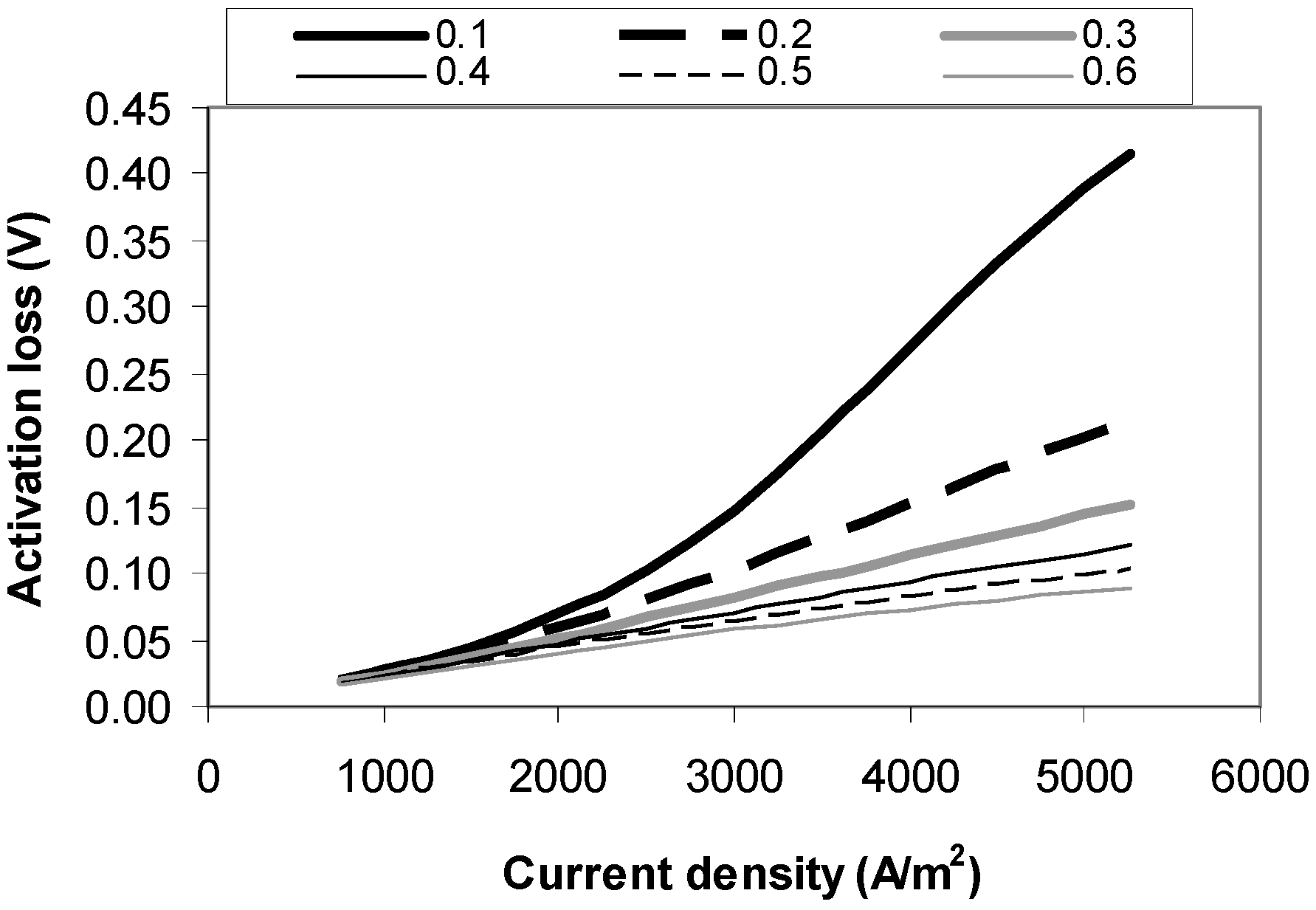
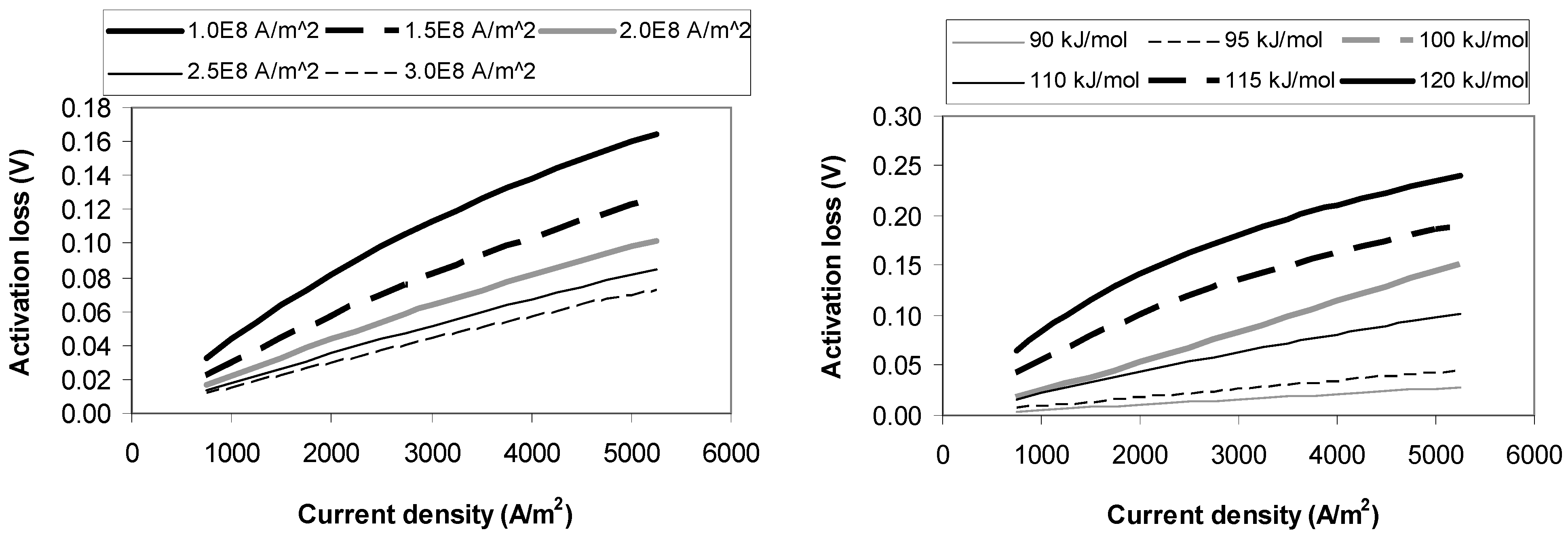
4.1. Activation Loss Sensitivity Analysis

There are three main user specifiable inputs to the activation loss model; the exchange current density constants, activation energies used to calculate the exchange current densities, and the transfer coefficient used within the Butler-Volmer equation. Both the anode and cathode activation losses are determined using the same type of equations (Equations 12, 13, and 14), therefore the influence of the input parameters on the losses are the same. For this reason, only the anode results are presented.

Figure 1a and Figure 1b show the dependency of the anode activation loss on the exchange current density constant and the activation energy, E, respectively. As it can be seen, the activation loss is heavily dependent on the activation energy, thus its correct value as an input parameter is crucial for accurate SOFC modeling. [13] proposed a value of 110 kJ/mol for both anode and cathode, while [11] presented values for the anode and cathode of 100 and 120 kJ/mol, respectively. The exchange current density constant has a smaller influence on the activation loss than the activation energy, but its value is still important when specifying the operating point of the SOFC.

The dependency of the activation loss on the transfer coefficient is shown in Figure 2. As it can be seen, with the values of the transfer coefficient below 0.2, the activation loss increases significantly. The transfer coefficient must by theory be in the range of 0–1, and has experimentally been found to be approximately 0.5 [16]. In the literature, when fitting the model results to the available experimental data, the anode value is usually taken as 0.5, while the cathode value varies in the range of 0.1–0.6 [3,12].

Figure 1. (a) (Left) Dependency of activation loss on exchange current density constant (b) (Right) Dependency of activation loss on activation energy.

Figure 1. (a) (Left) Dependency of activation loss on exchange current density constant (b) (Right) Dependency of activation loss on activation energy.

Figure 2. Dependency of activation loss on charge transfer coefficient.

Figure 2. Dependency of activation loss on charge transfer coefficient.

In all the above figures, it is important to note that the activation loss is steadily increasing with current density, and is a contributing loss over the entire range of current densities investigated.

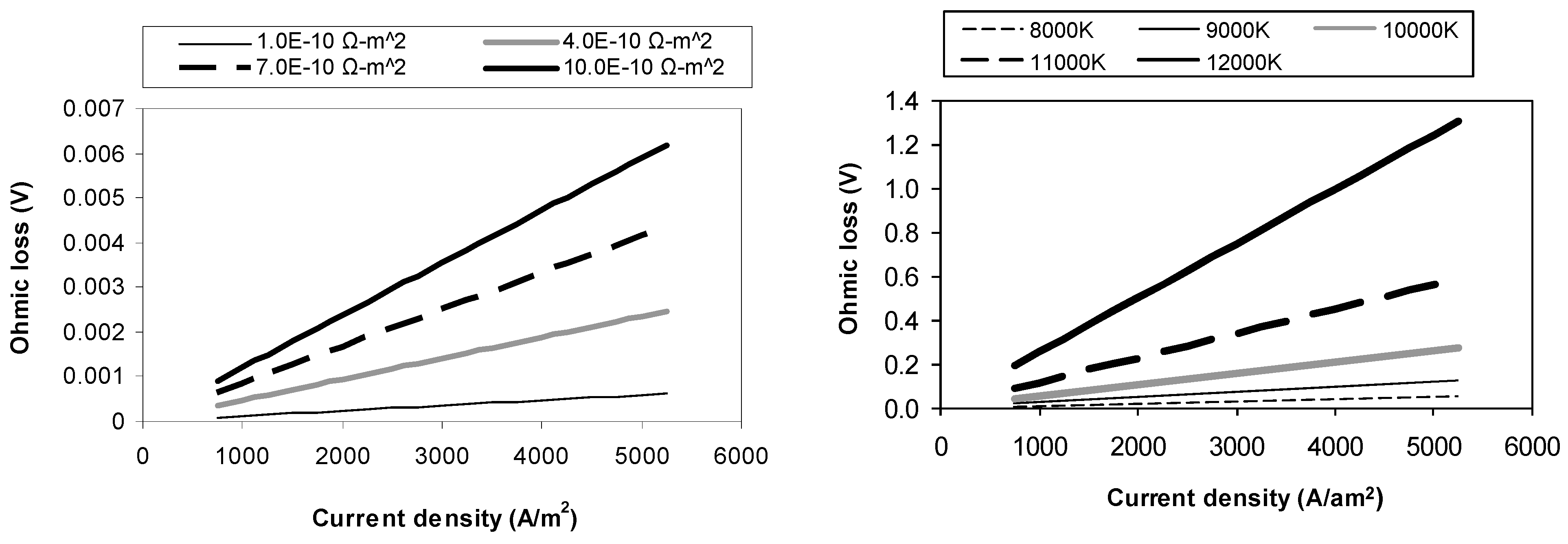
4.2. Ohmic Loss Sensitivity Analysis

The ohmic loss depends on the material properties of the electrodes, electrolyte and the interconnects. In this study, overall values were assumed eliminating the need to know the specific dimensions of the fuel cell. Figure 3a and Figure 3b show the dependency of the ohmic loss on constants A and B used to calculate the total resistance within the SOFC. As it can be seen, the ohmic loss is linearly dependent on the value of constant A, while it is exponentially dependent on constant B. At values above 10,000 K, the ohmic loss increases rapidly, and an increase of 10% from 10,000 K to 11,000 K increases the ohmic loss by more than 115% at a current density of 3,000 A/m². When fitting the model to experimental data, the temperature dependence of the model can be adjusted by adjusting the constant B.

Figure 3. (a) (Left) Dependency of Ohmic loss on constant A (b) (Right) Dependency of Ohmic loss on constant B.

Figure 3. (a) (Left) Dependency of Ohmic loss on constant A (b) (Right) Dependency of Ohmic loss on constant B.

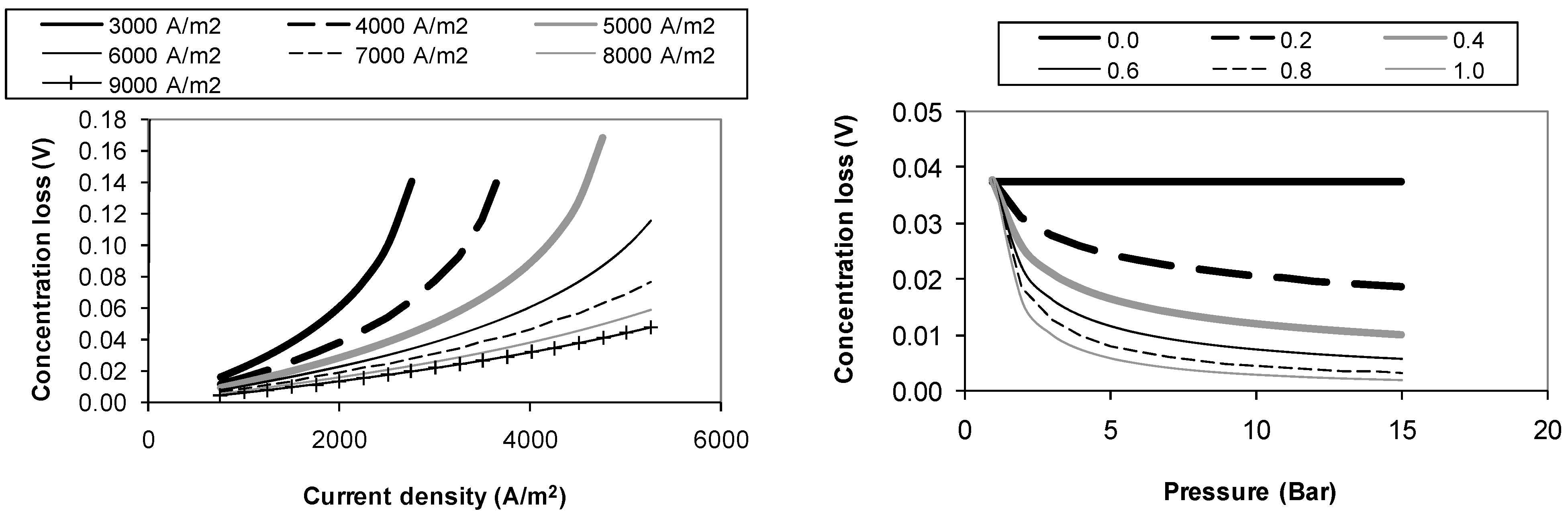
4.3. Concentration Loss Sensitivity Analysis

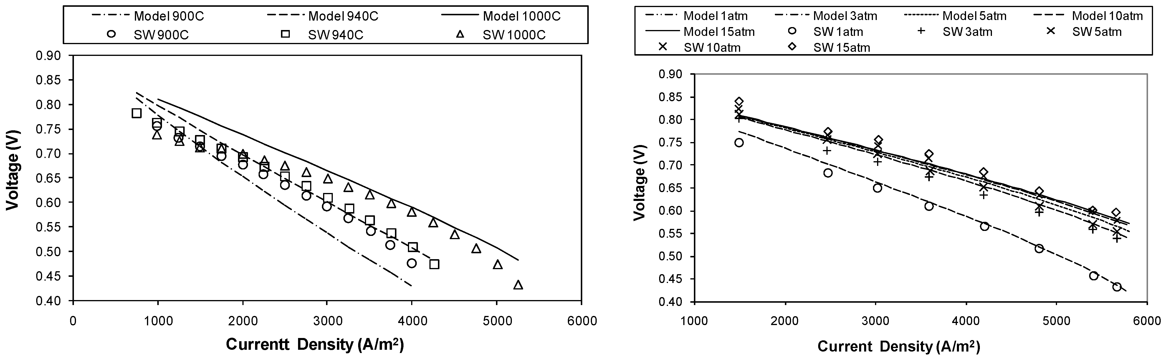
The concentration loss is heavily dependent on the limiting current density. In a fuel cell, the reacting species are reacted by the anode and the cathode, which give rise to local concentration drops with respect to the bulk air and fuel streams. The current density at which the rate of reactant flow from the bulk streams to the electrodes is not high enough to feed the reaction is called the limiting current density. In Figure 4a, the effect of the limiting current density on the concentration loss is shown. As the limiting current density approaches the actual current density, the concentration loss shows an asymptotic behavior, e.g., for the curve i_L = 6,000 A/m², the asymptotic behavior can be observed as the current density approaches 6,000 A/m².

Figure 4. (a) (Left) Dependency of concentration loss on limiting current density (b) (Right) Dependency of concentration loss on correction factor.

Figure 4. (a) (Left) Dependency of concentration loss on limiting current density (b) (Right) Dependency of concentration loss on correction factor.

Figure 4b shows the influence of the limiting current density correction factor on the concentration loss over a pressure range of 1–15 bar, at a constant operating current density of 3,200 A/m². Without the correction factor (a = 0.0), the concentration loss stays constant over the entire pressure range. With a correction factor, it is possible to account for the pressure dependency of the concentration loss. As the correction factor is increased, the change in the concentration loss decreases. Because the correction factor effectively represents increasing limiting current densities with pressure, this behavior can be explained from the small changes in concentration loss in Figure 4a for high values of the limiting current density.

5. Model Validation

Using the sensitivity analysis presented above, the model constants were tuned using the experimental data from Siemens Westinghouse as presented in [1]. The experimental data was for a tubular SOFC, 1.5 m active length, fed with 89% H₂–11% H₂O fuel using air as the oxidant. For the simulation of the temperature and pressure dependency of the model, four and six times the stoichiometric amount of air was used, respectively, as in the case of experiments.

The model was run using the input values given in Table 1, fed with a fuel composed of 89% H₂–11% H₂O, and air composed of 21% O₂–79% N₂. The resulting outputs, along with the experimental results of the Siemens Westinghouse tubular SOFC are given in Figure 5a and Figure 5b.

Figure 5a shows the temperature dependency of the model and experimental cell at atmospheric pressure. There is an acceptable qualitative agreement between simulation result and experimental data especially at medium and high values of the current density. The experimental voltage data is generally lower than the simulated results at low temperature (900 °C). In Figure 5b, the voltage-current density dependency on pressure is illustrated at a temperature of 1000 °C. There is a good qualitative match between the experimental and simulated results for the entire pressure range. At conditions other than those covered by Figure 5, it is not certain how well the results of the SOFC model would match the performance data of an actual fuel cell due to lack of available experimental data.

Figure 5. (a) (Left) Dependency of operating voltage on temperature (b) (Right) Dependency of operating voltage on pressure.

Figure 5. (a) (Left) Dependency of operating voltage on temperature (b) (Right) Dependency of operating voltage on pressure.

6. Conclusions

A macro-level model of a SOFC was developed, upon which a sensitivity analysis on different input parameters was performed. Using the results of the sensitivity analysis, the model was validated with experimental data from a Siemens Westinghouse tubular SOFC. For a single set of parameters, the model was able to match the experimental data well.

References

1. Singhal, S.C.; Kendall, K. High Temperature Solid Oxide Fuel Cells; Elsevier: Oxford, UK, 2003. [Google Scholar]
2. Power Generation. Available online: http://www.powergeneration.siemens.com (accessed on 15 November 2010).
3. Larminie, J; Dicks, A. Fuel Cell Systems Explained; Wiley: New York, NY, USA, 2004. [Google Scholar]
4. Omosun, A.O.; Bauen, A.; Brandon, N.P.; Adjiman, C.S.; Hart, D. Modeling system efficiencies and costs of two biomass-fuelled SOFC systems. J. Power Sources 2004, 131, 96–106. [Google Scholar] [CrossRef]
5. Pfafferodt, M.; Heidebrecht, P.; Stelter, M.; Sundmacher, K. Model-based prediction of suitable operating range of a SOFC for an Auxiliary Power Unit. J. Power Sources 2005, 149, 53–62. [Google Scholar] [CrossRef]
6. Palsson, J.; Selimovic, A.; Sjunnesson, L. Combined solid oxide fuel cell and gas turbine systems for efficient power and heat generation. J. Power Sources 2000, 86, 442–448. [Google Scholar] [CrossRef]
7. Song, T.W.; Sohn, J.L.; Kim, J.H.; Kim, T.S.; Ro, S.T.; Suzuki, K. Performance analysis of a tubular solid oxide fuel cell/micro gas turbine hybrid power system based on a quasi-two dimensional model. J. Power Sources 2005, 142, 30–42. [Google Scholar] [CrossRef]
8. Yakabe, H.; Ogiwara, T.; Hishinuma, M.; Yasuda, I. 3D model calculation for planar SOFC. J. Power Sources 2001, 102, 144–154. [Google Scholar] [CrossRef]
9. Roos, M.; Batawi, E.; Harnisch, U.; Hocker, T. Efficient simulation of fuel cell stacks with the volume averaging method. J. Power Sources 2003, 118, 86–95. [Google Scholar] [CrossRef]
10. Lazzaretto, A.; Toffolo, A.; Zanon, F. Parameter setting for a tubular SOFC simulation model. J. Energ. Resour. Technol. 2004, 126, 40–46. [Google Scholar] [CrossRef]
11. Costamagna, P.; Selimovic, A.; Del Borghi, M.; Agnew, G. Electrochemical model of the integrated planar solid oxide fuel cell. Chem. Eng. J. 2003, 102, 61–69. [Google Scholar] [CrossRef]
12. Noren, D.A.; Hoffman, M.A. Clarifying the Butler-Volmer equation and related approximations for calculating activation losses in solid oxide fuel cell models. J. Power Sources 2005, 152, 175–181. [Google Scholar] [CrossRef]
13. Calise, F.; Palombo, A.; Vanoli, L. Design and partial load exergy analysis of hybrid SOFC-GT power plant. J. Power Sources 2006, 158, 225–244. [Google Scholar] [CrossRef]
14. Freeh, J.E.; Pratt, J.W.; Brouwer, J. Development of A Solid-oxide Fuel Cell/gas Turbine Hybrid System Model for Aerospace Applications. In Proceedings of the ASME Turbo Expo 2004, Vienna, Austria, 14–17 June 2004.
15. Kuchonthara, P.; Bhattacharya, S.; Tsutsumi, A. Energy recuperation in solid oxide fuel cell (SOFC) and gas turbine (GT) combined system. J. Power Sources 2003, 117, 7–13. [Google Scholar] [CrossRef]
16. Hoogers, G. Fuel Cell Technology Handbook; CRC Press: New York, NY, USA, 2003. [Google Scholar]