Relating Financial and Energy Return on Investment

Abstract
: For many reasons, including environmental impacts and the peaking and depletion of the highest grades of fossil energy, it is very important to have sound methods for the evaluation of energy technologies and the profitability of the businesses that utilize them. In this paper we derive relations among the biophysical characteristic of an energy resource in relation to the businesses and technologies that exploit them. These relations include the energy return on energy investment (EROI), the price of energy, and the profit of an energy business. Our analyses show that EROI and the price of energy are inherently inversely related such that as EROI decreases for depleting fossil fuel production, the corresponding energy prices increase dramatically. Using energy and financial data for the oil and gas production sector, we demonstrate that the equations sufficiently describe the fundamental trends between profit, price, and EROI. For example, in 2002 an EROI of 11:1 for US oil and gas translates to an oil price of 24 $2005/barrel at a typical profit of 10%. This work sets the stage for proper EROI and price comparisons of individual fossil and renewable energy businesses as well as the electricity sector as a whole. Additionally, it presents a framework for incorporating EROI into larger economic systems models.1. Introduction
What is the minimum energy return on energy invested (EROI) that a modern industrial society must have for its energy system for that society to survive? To allow a profitable business venture? To afford arts, culture, education, medical care? To grow? Is it the same as the minimum EROI that a fuel must have to make a meaningful contribution to a society's material well-being? And what is the price of energy at this minimum EROI? There has been remarkably little discussion of this issue in the last 50 years outside of our own previous papers on the subject [1] even though we believe that it might be a defining aspect of future societies. Many earlier authors, including anthropologist Leslie White [2], economist Kenneth Boulding [3], anthropologist/historian Joseph Tainter [4,5] and ecologist Howard Odum [6] have argued that for a society to have cultural, economic and educational richness it must have a large quantity of energy resources with sufficient net energy. That is to say complex societies need a high EROI built on a large primary energy base.
With the exception of the considerable discussion around whether corn-based ethanol is or is not a net energy yielder [7,8] there has been almost no contemporary discussion of the implications of changing EROI on industrial society. The lack of such studies seems curious as this will be a very important issue relating to our future, during which the mutual impacts of peak oil and declining EROI of fossil resources are likely to cause a very large overall decline in the net energy delivered to our industrial society. Furthermore, a lack of consistent and sufficient net energy comparisons among fossil fuels and renewable energy alternatives for liquid fuels and electricity prevents adequate understanding of our investments in alternative energy systems with different EROIs. This issue is exacerbated by the failure of the public at large, the media and even most of the scientific community to be able to see through the generally self-serving and shallowly analyzed pronouncements of various energy possibilities. For example, a wind farm and coal-fired power plant with equal EROI are not fully equal in terms of providing the same energy service until the wind farm is as dispatchable (on minute to daily time scales) as the coal plant. Additionally, a coal-fired power plant has more long-term uncertainty in EROI than a wind farm based upon the mining energy requirements. The wind farm long term certainty stems from the fact that the average wind speed will occur over the decadal life span of the turbines. Of course, environmental impacts and externalities (e.g., equivalent CO2 emissions) also could play a major role, but we restrict the scope of this paper to the pure energy economic implications of changing EROI. If in the future environmental externalities are priced into the economic market, our general methodology would still hold, but will need to be updated.
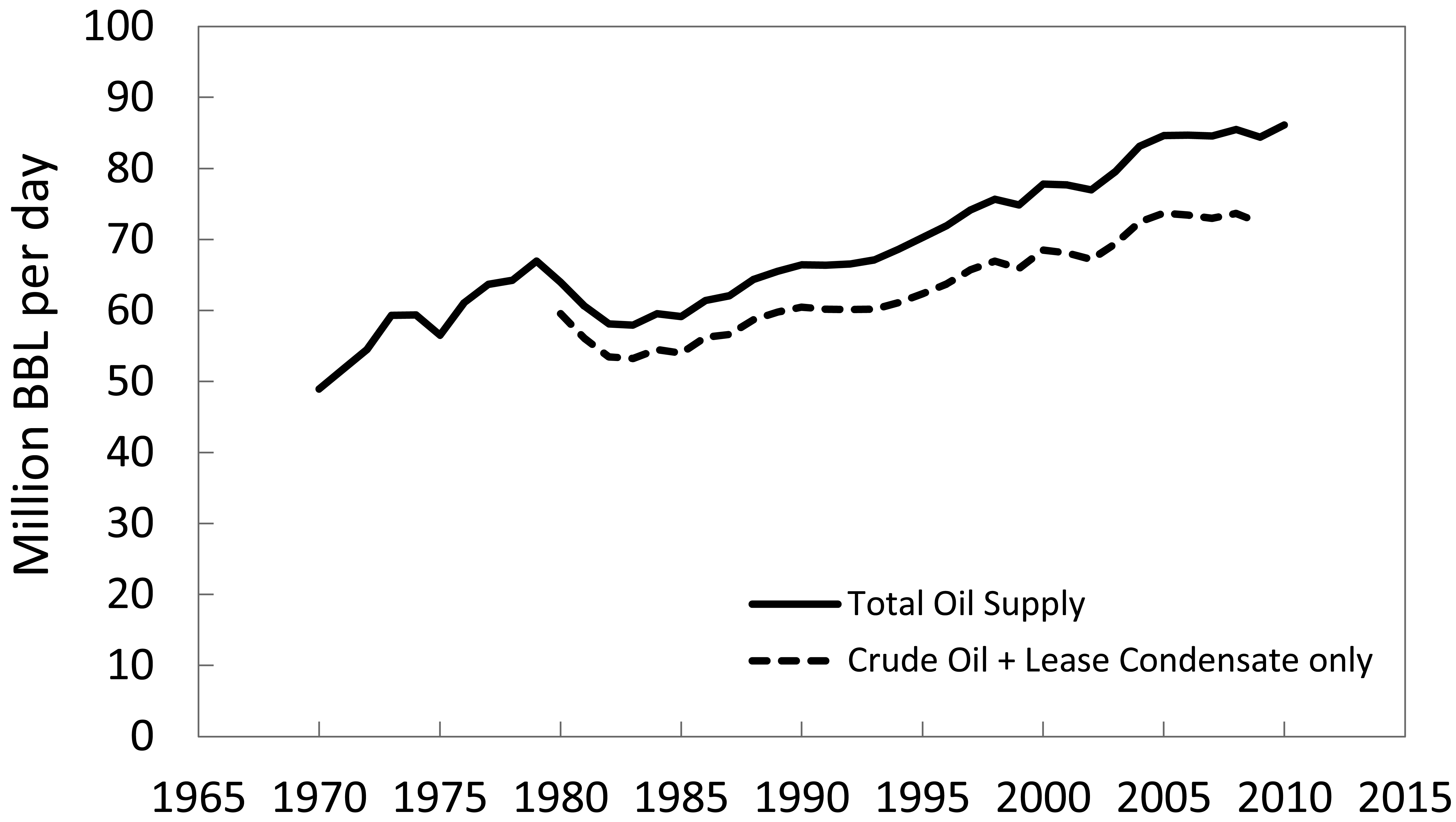
There may already be very large impacts of declining EROI on our society, although this is difficult to untangle from peak oil impacts and the recession that started in 2007, which was at least partly due to increasing oil price [9,10]. Whatever the particular causative chain of events, a few recent trends appear: both oil and energy use have been declining in the United States, including a drop in total energy consumption from 99.3 quads in 2008 to 94.6 quads in 2009 [11,12]; global peak crude oil production-or something like it has occurred or is occurring (see Figure 1) [13,14] with many agreeing that world crude oil production peaked in 2005; the US's “Great Recession” officially lasted from December 2007 until June 2009 [15]; many financial entities are still in very rough shape after the financial crises that began in 2008, including many banks and Wall Street firms; the average inflation-corrected value of stocks has ceased increasing over the last decade [10], bonds have outperformed stocks over the last decade; and over the last two years most States and many municipalities have been forced to cut social and civil services to balance budgets. To what degree all of these effects are related to EROI is speculative, but worth speculating on.
The most explicit analysis of the EROI needed by society that we are aware of is Hall, Balogh and Murphy (2009) [1]., who made calculations on the energy required to refine, ship and transport fuels to their use destination, as well as to develop and maintain the infrastructure necessary to use them They used direct and indirect energy costs (EROIstand) as recommended by Murphy and Hall in this special issue [16]. They concluded that the minimum EROI required for transportation fuels appeared to be in the vicinity of 3:1. That is to say, for every unit of energy consumed at the point of use, as in a car, at least three units of energy must be produced in order to (1) extract, refine and distribute the final fuel to the point of use in the form required by consumers, (2) manufacture the end-use machinery, and (3) build and maintain the infrastructure (i.e., roads and bridges) within which the fuel system operates. If the EROI was less than 3:1, then the fuel might be extracted but it could not be used to drive a transportation system. But this appears not to be the whole story.
No energy-producing entity (EPE, i.e., firm, National Oil Company, etc.) can produce a fuel over time (without subsidy) if it does not make a monetary profit, and it is not an EPE if it has a long-run EROI < 1:1. In other words, an EPE has the economic profit constraint of any other firm, so that it must sell its product (energy) for more than the monetary cost of the energy (direct and indirect) inputs required to produce it—plus it has to pay for the labor, profits and so on for the entire supply chain leading to the energy containing products it uses. These cost factors are normally accounted for in cash flow analyses of energy production businesses and processes, but are not always accounted for in EROI analyses. If we have a value for EROI that correlates to the same monetary costs of the full supply chain for energy production, then we should be able to estimate the cost of energy.
But the financial constraints are even stricter. For a firm to make a profit, it has to have some value of positive EROI because the energy flows associated with its costs (roughly 14–20 MJ per $2005 for the US oil and gas extraction industry, including direct and indirect costs [17,18]) are much less than the energy associated with a dollar's worth of its product. For example, if oil sells in 2005 for $61 per barrel (BBL) (containing 6,100 MJ), then each dollar gained by the oil company is associated with 100 MJ that has come out of the ground. If the EROI for the oil was 2:1, then the firm could not make a profit because for each 20 MJ invested in the business, at a cost of $1, only 40 MJ are output can be sold at a value of $0.40 [19]. Hence, at $61/BBL to make a profit a firm needs to have an EROI of at least 5:1, or alternatively if the price of oil were higher the firm could make a profit at a lower EROI. The conundrum is that as the price of oil goes up so does, historically, the price of everything else, at least eventually, including those things required to produce the oil. For example, cost for drilling US oil wells increased 270% from $150/ft in 2000 to $590/ft in 2007 (in $2007) [20] as the US first purchase price of oil increased 110% from $30/BBL to $63/BBL (in $2005) during the same time frame [21]. Over time the minimum EROI for a profit can be used as an investment guide for the company.
Our objective in this paper is to relate the EROI of energy produced by an EPE to the cost of energy and monetary return on investment (MROI) of that same firm, both theoretically and compared to historical empirical information for US energy sectors. This is not merely an academic exercise. As the EROI of our major fuels continues to decline [18,22] a major extension of this analysis is that economic profitability could stop long before EROI reaches 1:1. Our hypothesis for the analysis of this paper is that the biophysical characteristics of producing available energy, namely the EROI of the energy production process, dictate a limit on the price and profit margin for a firm to engage in energy production and exploitation. At least one other paper has addressed the important issue of relating EROI to price of energy, where the authors applied a statistical analysis of various fitted curves that are based upon a similar structure as we present [23]. Here, rather than optimize for a statistical correlation, we formulate an underlying basis for the relationship between price and EROI such that there is a physical basis for price and a framework for projecting future trends.
2. Methods
Our basic method was to develop a mathematical expression for the relation of the biophysical characteristic, EROI, of an exploitable energy resource to the economic conditions that makes the exploitation possible. We derive an equation that describes the general trends of certain parameters of interest, namely the EROI, the monetary return on investment (MROI), and the unit price of produced energy, p (e.g., $/BBL, $/MWh, etc.) sold in the market. At MROI = 1, the predicted price equals the producer price, or cost of production.
The definition for EROI is as shown in (1). EROI is the energy output (Eout) from an energy production system divided by the required energy inputs (Ein) to the system. Most EROI analysts calculate (1) without discounting future energy production versus energy produced and consumed today, and for simplicity, our analysis also assumes simple energy and cash flow accounting (i.e., we do not discount energy or money) [24].
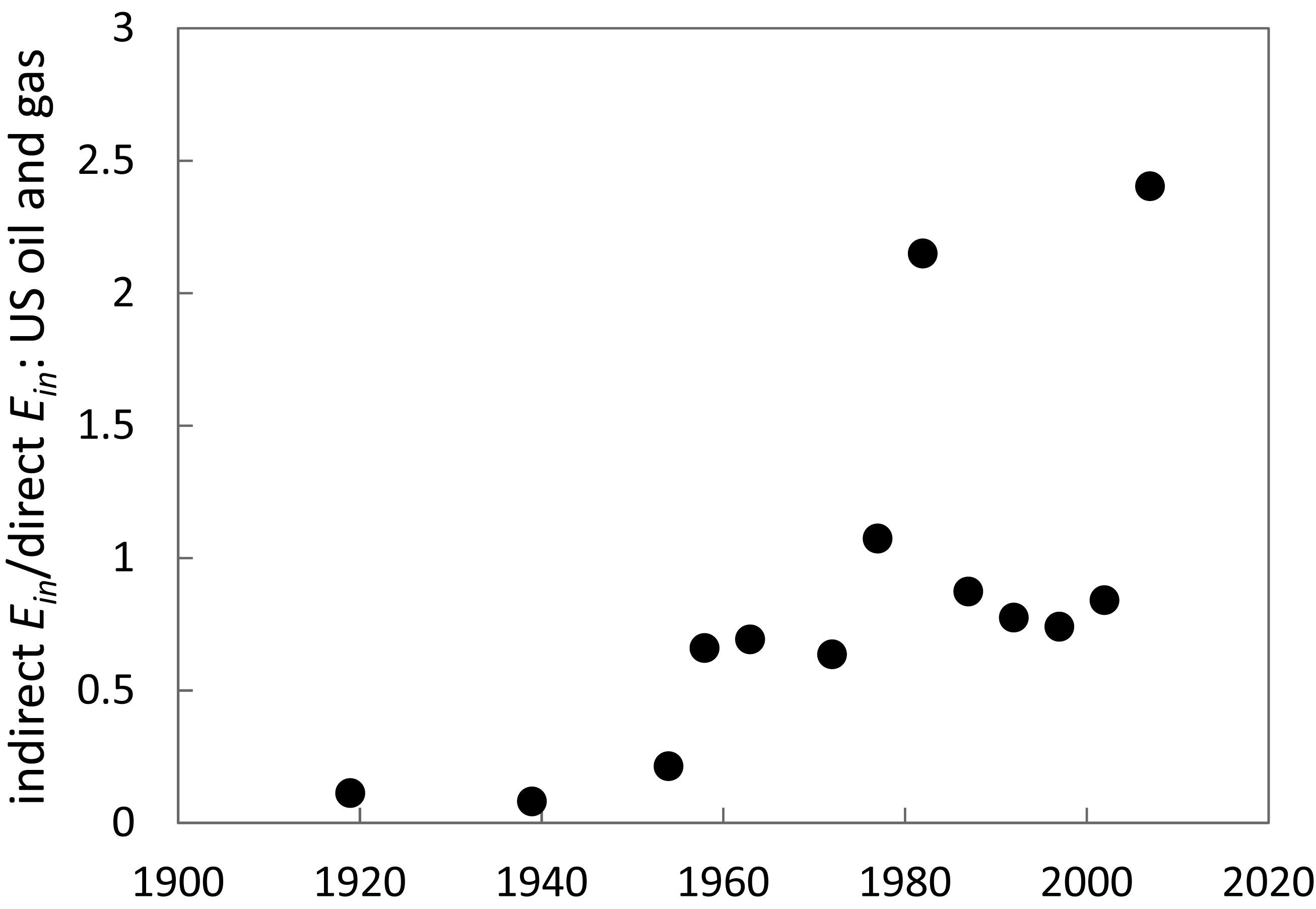
Most analyses also imply that the relation for investments today are reflecting production today, whereas today's production is partly from yesterday's capital investments and today's capital investments are partly for tomorrow's production. The data from [18] used in this paper indicate that the ratio of indirect indirect Ein/direct Ein for US oil and gas has varied from less than 0.3 to over 2 in the years in which high oil prices induced large increases in exploration and drilling (see Figure 2).
We now deconstruct (1) into a form used to calculate results for this paper. However, for previous descriptions of the general framework for characterizing how to include different inputs and outputs in (1), see [25-29]. Note that both the numerator and denominator of (1) can be composed of multiple factors: M forms of energy outputs and N forms of energy inputs. For example, an analysis of a drilling operation producing oil, natural gas, and natural gas liquids must count the energy content of all three (e.g., M = 3) resources to calculate Eout. The same premise holds for calculating Ein. Relations for the energy outputs and inputs of an energy production system are shown in (2) and (3) as a function of energy intensity, ei of production (or consumption), multiplied by the number of units of production (or consumption). Here, we assume ei is expressed in units of energy divided by any other unit whether that by a physical quantity (e.g., tonnes), money (e.g., dollars), or otherwise. In (2), M is the number of output energy products, and mi represents the unit production of the ith energy product. In (3), N is the number of input products that have direct or indirect embodied energy, and ni represents the unit consumption of the ith input. Example units of energy production are barrels (BBLs) of oil, megawatt-hours (MWh) of electricity, thousand cubic feet (MCF) of natural gas, etc. An example calculation is Eout for oil production where the energy content of a barrel (BBL) of oil is approximately e= 6.1 GJ/BBL, and if m = 10 BBLs of oil are produced, then Eout = 61 GJ. For Equation (3), the ith unit input can describe direct energy (e.g., a BBL of oil) or indirect energy (e.g., energy embodied in a ton of steel, hour of labor, etc.). See [25] and [30] for a full discussion of how to consider different energy inputs and outputs, including using energy quality factors, when calculating Ein and Eout.
Equation (3) should include both direct and indirect energy inputs and represents the common methodology for performing process-based and input-output based life cycle assessments (LCAs) [31]. Hence with proper data we can assess what part of the expenditure dollar went for direct energy and what part for the indirect energy that is responsible for the different energy/monetary ratios of inputs and products. For example, in an oil production system, the direct Ein calculated in (3) can be a summation of electricity (or better the fuel consumed during electricity generation) for running trailers, pumps, compressors, and computer equipment as well as diesel fuel consumed for operating trucks, pumps, and the drilling rig. However, it is insufficient to include only the direct energy inputs to capture all of the energy necessary for the full operation of the energy production system. EROI researchers additionally include measures for indirect energy inputs to consider energy inputs from operations outside of the energy producing operation itself. For example, oil derricks have towers made from steel, and one company may install and operate the drill, but another made the steel tower. Because the energy inputs required to make the steel are not performed on the site of the oil well, they are considered indirect energy and can be included in the analysis by knowing the energy required per unit or dollar of production (e.g., energy intensity e) and following (3). For example, in 2004 the average mass energy intensity of steel was est = 20,000 MJ/tonne [32]. Thus, to include the indirect energy inputs from steel in (3), n is number of tonnes of steel and ei = est = 20,000 MJ/tonne. When physical units are not available analysts must use dollars of steel (e.g., n in units of $) and monetary energy intensity (e.g., e in units of MJ/$) for such dollars spent.
It is possible to estimate indirect Ein using nominal data from input-output (I-O) analyses of the entire economy. Examples of such analyses are those by Bullard, Herendeen, and Hannon in the 1970s [33], Costanza and Herendeen in the 1980s [34,35], and the somewhat less comprehensive or detailed but more recent Economic Input-Output LCA analyses by Carnegie Mellon [36]. These I-O analyses blend national-level economic and energy consumption data to analyze the impacts of complete economic sectors rather than individual technologies or processes. In using I-O analyses, the most aggregated value of ei that characterizes energy consumption and economic cost is the economy-wide energy consumed for every one dollar of investment by the energy sector of interest (e.g., oil and gas extraction sector). If monetary ei (e.g., in units of MJ/$) is not available for the sector or project of interest via an I-O analysis, then the overall monetary energy intensity, e, of the economy (e.g., state, country, world) can be used as the best proxy. However, investments of energy industries have higher than average energy intensity. Equation (4) represents energy inputs as a function of money invested and energy intensity of the investment, einvestment, in units of energy per money (e.g., MJ/$).
Alternatively, one can calculate einvestment using Equation (3) to calculate all energy inputs and dividing them by all money spent to purchase those inputs. For reconstructing the value of einvestment without I-O analyses, we can use (5).
To relate EROI to the einvestment, we substitute (2) and (4) into (1) to obtain (6), a working definition of EROI.
Thus, the higher the einvestment for energy business operations, the lower the EROI. Note that in the case of oil production, as the oil resources left to exploit get deeper, heavier or from more inhospitable areas, it is important to understand not only how much more direct energy (e.g., diesel fuel and electricity) is required for drilling deeper and pumping up the oil but also how much indirect energy (e.g., infrastructure, engineering, and planning) is required. If an oil resource primarily requires direct energy, this raises einvestment because fuels have high ratios of energy/$ by definition (e.g., if a fuel was sold for an energy/$ ratio below that of the average of the economy, then the firm selling the energy would be a net energy consumer and not a net energy producer). Therefore, as einvestment increases, this produces a further feedback on decreasing the EROI of the resource. Additionally, the steel, aluminum, and other heavy manufacturing materials that are required for new drilling and construction of power plants are also characterized by einvestment higher than economy average (but lower than for fuels), again creating a feedback for lowering the EROI per Equation (6).
We next create (7), where mi are in physical units of produced energy and ei are in units of as an analog to (6) to enable a relation between simple monetary return on investment, MROI and EROI.
From (7), we solve for the total money invested as:
Substituting (8) and (5) into (6) and we obtain an equation that shows EROI as a function of important economic factors:
We use Equation (9b) to explicitly solve EROI as a function of the individual components of einvestment. Assuming for simplicity that there is only one type of energy production (e.g., M = 1), we easily solve (9) for one output variable of interest as a function given values for all other variables. For example, useful relations are (10) and (11). Equation (10) specifies the requisite sales price, p, of a unit of energy production (e.g., $/BBL of oil) as a function of EROI and MROI, and (11) specifies the monetary return on investment as a function of EROI. In the following results section, we use (10) and (11) to demonstrate the current methodology.
The benefit of the relations described by (4–11) is that we have derived an equation with both EROI and MROI explicitly stated together. Previous research either defines EROI without relation to monetary profits, or derives EROI from economic data of a specific year, but still without a closed form function relating EROI and MROI. To properly use (10) and (11), one must make sure that the parameters all correspond to the same time frame and system boundaries or point in the supply chain of an energy production technology, business, or system. For example, if analyzing the price of oil from a specific field, then the inputs to (10) and (11) must be the expected MROI, EROI, and einvestment of production for that field only. If one is interested in the average price of oil from the entire United States oil and gas sector, then the inputs to (10) and (11) must relate to the entire sector. Thus, the structure of ((4)–(11)) should allow researchers to do both top-down economic sector analyses as well as bottom-up technology-specific analyses to analyze the entire energy supply chain. By reconstructing the top-down results from bottom-up techniques, better future energy projections may be possible. However, in practice, bottom-up process LCAs are more easily performed using Ein as defined in (3) because values for process-specific einvestment are generally not available.
In ((9)–(11)) the various factors are not independent of each other. Ideally, data and calculations for EROI can be made independent of economic inputs, and this is most plausible when considering direct energy inputs only in (3). In considering indirect energy inputs, however, (e.g., that energy required for producing steel used in oil well casing), often times only monetary data are available (e.g., money spent for purchasing steel), requiring a blend of available economic and energy intensity data (e.g., an aggregate value of e in units such as MJ/$) to estimate energy inputs. Additionally, when considering sector level analysis, economic data are generally all that are available. Thus, it is important to understand that EROI is not an independent function of einvestment as it appears to be considered in ((9)–(11)). For example, oil as refined diesel is a major input into drilling for oil (e.g., as fuel for drilling rigs). Thus, if the biophysical descriptor (i.e., EROI) decreases because of the need to consume more diesel in drilling to deeper oil resources, other input products (e.g. steel) can become more expensive in both money and energy if they depend upon oil for production and shipping. That is to say, as the price of oil gets higher, it can have a feedback making it more expensive to produce more oil. Additionally, EROI is inversely proportional to the energy intensity of investment in energy production while at the same time being proportional to the energy output per unit of production (e.g., BBLs of oil production at 6,100 MJ/BBL). By using (9), we can account for a situation in which the EPE pays a price for an energy resource input that is different than the price for which the EPE sells the same energy resource as an output. By breaking einvestment into a weighted sum of many investments as in (5) and (9), we can gain insight into the coupling of inputs from each sector or fuel (direct or indirect) upon EROI, and ultimately the price of energy required to make a given financial return. In practice such assessments often are very difficult because the energy companies (especially national oil companies) keep much of this information to themselves.
Also,Equations(10) and (11) show that as energy gets more expensive, partially characterized by decreasing energy intensity (e.g., energy per dollar) of investment in energy production, einvestment, then energy price increases at constant EROI. The counter-intuitive result from (10) is that as the energy intensity of investing in energy production increases, the price of energy necessary to make a constant profit decreases. The reason is that higher energy intensity purchases represent cheap energy inputs and the ability to make higher monetary returns for a given EROI.
3. Results
To gain insight into our methods, we use Equation (10) to estimate results under representative historic economic conditions. We first use the example of US oil production and later repeat the analysis for natural gas and coal production. Our results indicate that Equations (9–(11)) act as broad but valid representations of the relations between EROI, MROI, and the stated technoeconomic factors.
3.1. Calculating Oil Price as a Function of EROI and Financial Parameters
Assuming for the moment that barrels of oil are the only energy output unit from oil and gas operations, we use (10) to plot estimated oil price for a range of expected inputs. Equation (10) has four inputs on the right hand side, and we must choose sources of data for these data inputs. Because there are no definitive values to input into Equation (10) for calculating oil price, we calculate price as a function of EROI using a range of reasonable inputs. We estimate input values for estimating the price of oil via Equation (10) as follows and plot the results in Figure 2:
eoil:We assume that the energy content for a barrel of oil is 6,100 MJ/BBL.
einvestment: Per Equation (9b) energy inputs are a combination of direct and indirect energy. By summing all energy inputs and dividing by all monetary inputs we obtain the estimate for total einvestment. For estimating the total einvestment for oil and natural gas we use the direct and indirect energy input values from Guilford et al. (2011) of this special issue of Sustainability [18]. Reliable fuel price data (for cost of direct energy from natural gas, fuel oil, gasoline, and electricity) exist from the EIA after 1949, and we only calculate total einvestment for dates after 1949. Guilford et al. (2011) assume a nominal estimate of einvestment = 14 MJ/$2005 for cost of capital, or indirect energy inputs [18]. The Appendix shows the values for einvestment for each year of data in [18].
MROI: We use estimates of monetary return on investment, MROI, from two sources for comparison and sensitivity analysis: the EIO-LCA oil and gas extraction industry (NAICS 211) and a document of the American Petroleum Institute (API) [37]. The API quotes a 7% annual profit assumption for the entire oil and gas industry and is likely an underestimate, but represents a typical long term value. The EIO-LCA model specifies 40% and 51% annual profits for 1997 and 2002, respectively, for the targeted NAICS 211 oil and gas extraction sector producer price models [36,38]. Thus, we plot Equation (10) for both MROI =1.1 and MROI = 1.5 to signify the expected range of profits.
EROI: We plot estimates of EROI for US oil and natural gas from two sources alongside our results plotted using Equation (10) (see references below for discussions of how EROI varies over time):
The first EROI estimates are those of the US oil and gas industry from Cleveland (2005) reported for every fifth year from 1954 to 1997 [26], and
the second EROI estimates are those of the US oil and gas industry from Guilford et al. (2011) [18] of this special EROI issue for every fifth year from 1919 to 2007.
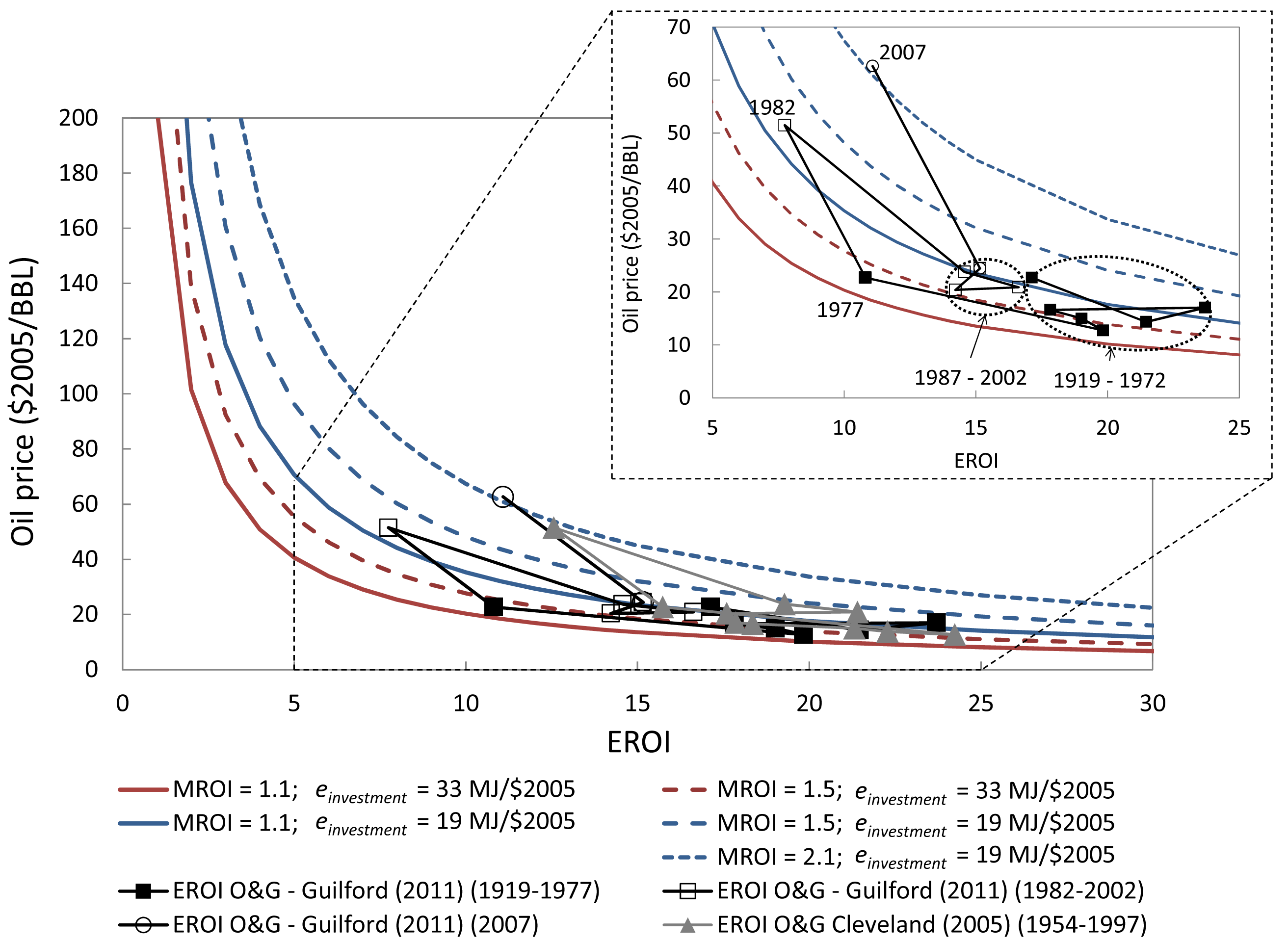
The most difficult factors to obtain accurately in (10) are the EROI and MROI for any given time period, and thus the methods of this paper should not be expected to predict short term price fluctuations, but rather they contribute insight into long term trends. For a given EROI, however, it is easy to see the price effect of the energetic cost of production and taking higher profits. In Figure 3 we plot the general trends of the price of a BBL ($2005/BBL) [21] of oil versus the EROI and expected range of MROI for the oil and gas industry. In recent history, EROI for oil and gas has been between 10–30 [22,26,28,39]. While this range appears to be large, it translates to an oil price of less than $70/BBL at annual profit ratios less than MROI = 1.5. This price has been exceeded regularly only in the last few years, which might reflect the apparently rapid decline in EROI that we have seen recently (see many papers in this special issue of Sustainability).
In Figure 3 the modeled range of oil price and EROI brackets most of the data points composed of literature EROI values and historical oil prices (only the average annual prices are plotted). Each solid and dashed line in Figure 3 represents the Equation (10) estimate and assumes a constant value for both einvestment and MROI. These data points confirm the general inverse trend of price relative to EROI. If EROI becomes less than 10, as may soon be the case for average US oil, the requisite oil price increases dramatically and at a nonlinear increasing rate. For example, consider the EROI of Canadian oil sands extraction that is now a significant source of petroleum and influential in setting the worldwide marginal oil price. Assume that each barrel of bitumen brought to the surface using steam assisted gravity drainage (SAGD) technique is 6,100 GJ/BBL, the same as crude oil (an overestimate). Additionally, assume a typical need for 2–3 BBL of steam per BBL of extracted bitumen and natural gas for creating steam at 0.45 Mcf/BBL of steam [40]. Using the natural gas as the first energy input (clearly not the only energy input) the EROI of oil sands is no larger than 4–6:1 nearly an order of magnitude lower than the average oil and natural gas EROI of the past. From Figure 3, we see that oil production with an EROI of 4–6 and annual profits between 10% and 50% requires a price of 40–120 $2005/BBL. Realistic EROI for oil sands near 3–4 indicate oil prices of 50–160 $2005/BBL: with the mid-range being higher than the economy was able to support running up to the recession started in late 2007 [15]. A review of oil shale in this special issue of Sustainability indicates that oil shale EROI is between 1 and 2.5 with the major energy input being direct energy for heating the shale [41]. Thus, our analysis suggests oil prices (at the mine) of $80/BBL–$200/BBL (in $2005) at 10% annual profit assuming the highest value of einvestment = 33 from Guilford et al. (2011; red solid line in Figure 3) [18].
In looking further at the plotted EROI and price points in Figure 3 we find an interesting pattern. Recall that the EROI values can only be calculated every fifth year due to data availability (see references for description). First, the EROI values from Cleveland (2005) predict higher prices at the same EROI [26]. Also, the only two outliers from the data points associated with oil prices less than 25 $2005/BBL are those for 1982 and 2007. The slopes are almost identical for the relative increase in price with decreasing EROI for both the price increase from 22.7 $2005/BBL in 1977 to 51.5 $2005/BBL in 1982 and also the price increase from 24 $2005/BBL in 2002 to 63 $2005/BBL in 2007. For the change from 1977 to 1982 the slopes are −9.1 and −9.4 (units of $2005 per EROI, or $2005) for Cleveland (2005) [26] and Guilford et al. (2011) [18], respectively. The slope from 2002 to 2007 is −8.3.
Each of the five lines plotted in Figure 3 using Equations (9) and (10) assumes a constant einvestment and MROI. The solid and dashed red lines (lower left lines) use einvestment= 33 MJ/$2005 which we calculated as typical for all years after 1958 except for 1982 and 2007. For both 1982 and 2007 our calculated einvestment =19 MJ/$2005. See the Appendix for details on calculating einvestmen.t. Assuming 10%–50% annual profit sufficiently describes the actual prices except for 1982 (Cleveland, 2005) [26] and 2007 (Guilford et al., 2011) [18]. During the time spans of 1979–1982 and 2005–2007 real oil prices rose more than $7/yr – too fast for oil companies to bring new production online to benefit from the prices. Thus, their existing production that planned on making a profit at lower prices made considerably larger profits (higher MROI than normal) during these years of abnormally high oil prices. Thus, Equation (10) and (11) as exhibited in Figure 3 show that oil prices in 1982 and 2007 allowed for significantly higher profits.
3.2. Calculating Natural Gas Price as a Function of EROI and Financial Parameters
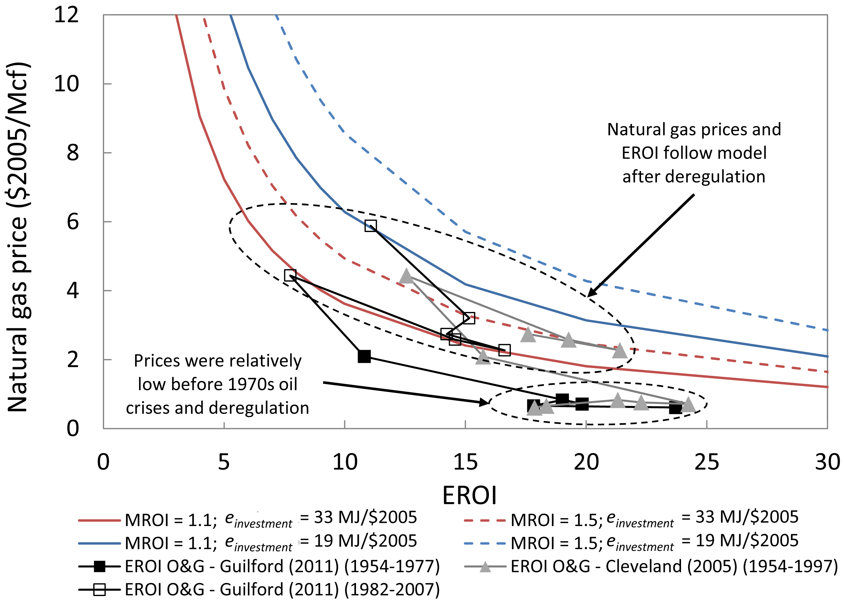
We repeated the calculations of Section 3.1 using natural gas as the output instead of oil (see Figure 4). We use eNG = 1,085 MJ/Mcf where Mcf is one thousand cubic feet of natural gas, the common US unit to describe natural gas transactions. We plot natural gas price ($2005/Mcf) [21] versus the same EROI for oil and gas from Cleveland (2005) [26] and Guilford et al. (2011) [18], and our relation again predicts the price trends relative to measured EROI. One important feature to notice in Figure 4 is the group of data points that lie below the bounds of the prediction Equation (10) and (11). These points correspond to prices and EROI for the year 1977 and earlier–before the Natural Gas Policy Act of 1978 ended regulation of wellhead natural gas prices. After 1977, natural gas producer prices rose to incentivize new production and more accurately reflect costs.
However, our results show the general ability of the basic formulation of the present work to relate EPE monetary and energy profits over long term trends. The formulation also shows that EROI < 10 generally relates to natural gas prices greater than 6 $/Mcf. Thus, it is very important to understand the EROI of new natural gas resources, such as from shales, because these are more decoupled from oil prices in accessing resources that do not coproduce natural gas with oil. Knowing the viable range of EROI for delivered, not wellhead, natural gas should help us gain understanding with regard to future volatility in natural gas prices.
3.3. Impact of Capital Intensive Energy Technology
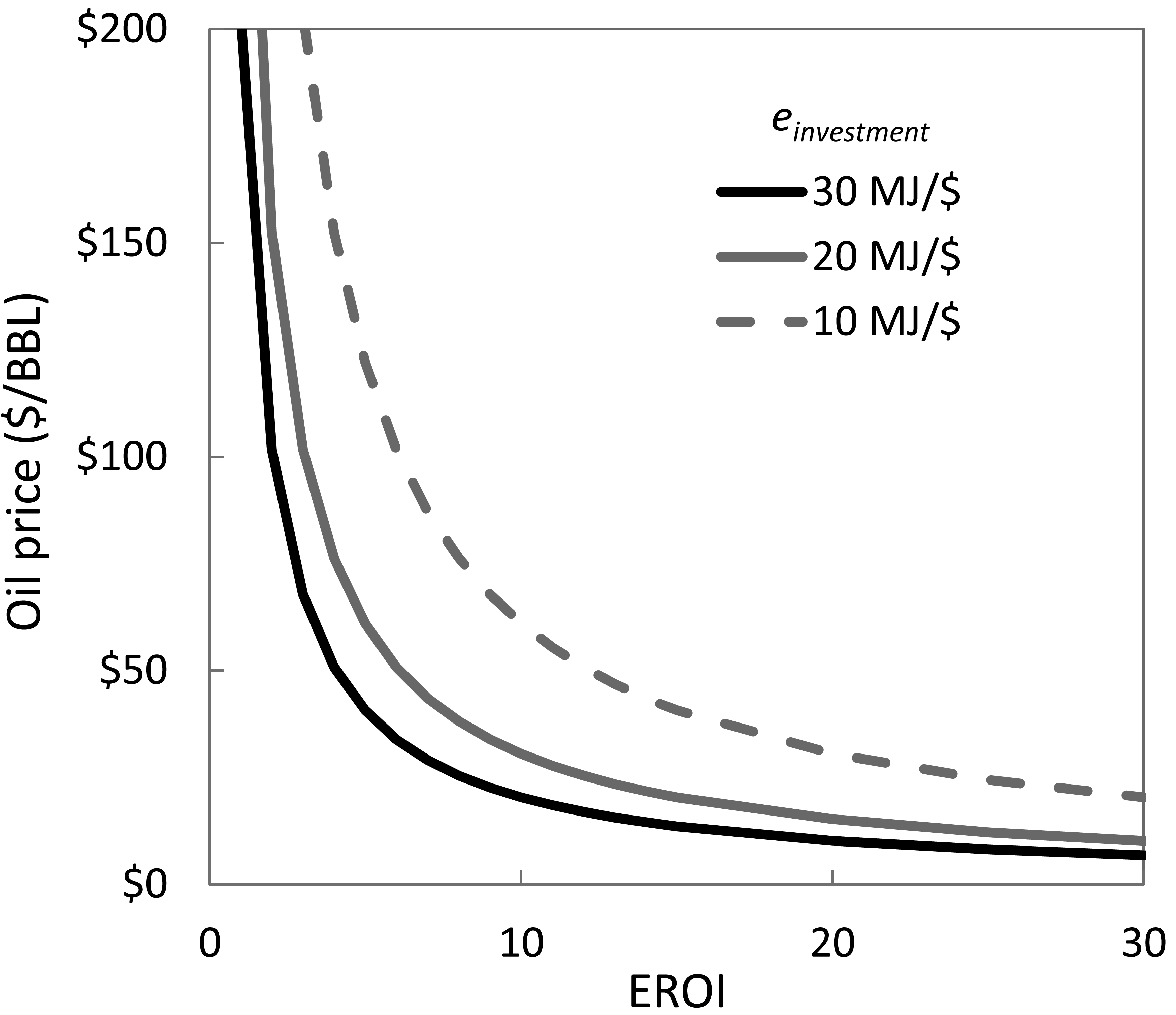
There is an interesting and important trend to note from our relation between price and EROI. This trend relates to the energy intensity of the investment, einvestment, for energy generation. A capital intensive investment will have relatively little fuel consumption but relatively high material usage, or capital. We interpret high capital intensity of the investment as a low value of einvestment. For example, steel has direct embodied energy of approximately 20 GJ/tonne and at $700/tonne represents an energy intensity of esteel = 28 MJ/$. On the other hand, a fuel intensive investment in the life cycle of energy production is represented by a high value of einvestment. For example, if natural gas were an input to an energy production life cycle at $7/Mcf, a typical medium-range price, the energy intensity of that investment translates to eNG =155 MJ/$. Thus, if einvestment is weighted toward fuels, it will be relatively large. If einvestment is weighted toward materials and capital, it will be relatively low.
As Equation (10) and (11) indicate, as the capital intensity of the energy technology investment increases, the price of energy sold must increase even at the same EROI (see Figure 5). In other words, if one technology can produce fuel at EROI =10 and einvestment =10 MJ/$ and another technology can produce fuel at EROI =10 and einvestment =15 MJ/$, then the fuel is cheaper from the latter technology. Philosophically this means that, at an equal EROI, energy production systems that are more dependent on their own product (e.g., fuels) are cheapest. This concept has implications for renewable energy technologies that are relatively capital intensive in order to extract energy from the sun and wind yet have little to no fuel consumption during operational part of the life cycle. As seen in Figure 2, capital intensity also is important for understanding prices in the fossil fuel extraction industry. The oil and gas industry responded to high oil prices by increasing drilling rates in the early 1980s and late 2000s and this translated to higher material and human capital intensive investment periods (e.g., steel, concrete, overhead for oilfield service companies, etc.). Because the benefits of these capital investments occur for many years after initial the expenditure, it is important for future work to properly characterize the time lags of EROI and Eout relative to capital intensive energy investments. Future work should also explore the energy intensity, einvestment, of alternative fossil and renewable fuels to understand which price curve of Figure 5 is more relevant for each fuel (e.g., oil sands that are heavily reliant on natural gas, biofuels using both free solar energy and fossil fuel inputs, etc.).
4. Conclusions
Our equations derived in this paper appear to predict rather well the basic relations among profits, prices, and EROI This formulation, however, is not meant necessarily to predict short term prices, but rather characterize broad relations and the ways in which we believe that EROI drives large scale financial phenomenon and long-term energy investments. It is important to note that Equations (9–11) represent equilibrium conditions with no constraints on any required inputs. In reality there can be shortages in global oil supply or quickly increasing demand of infrastructure for oil and gas development (e.g., drilling rigs) that raise prices much faster (in time) than indicated by the theory of this paper. Thus, the theory of this paper can be viewed as describing a lower bound on price as it relates to EROI.
The data used in Guilford et al. (2011) [18] and Cleveland (2005) [26] do represent some dynamics in supply and demand with regard to oil production. Because the underlying data from the US Census of Mineral Industries is reported only every five years, there are few conclusions we can make regarding the rate at which the underlying EROI changes on annual or monthly time scales. By the method and demonstrations developed in this paper we have confirmed our major hypothesis that the biophysical characteristic of EROI is a major factor that can dictate the profit margin and price necessary for a firm to engage in energy production. The relations in Equations (9)–(11) illustrate that lower EROI energy systems have less potential profitability for their businesses.
Over the long run, any energy producing entity must produce both a monetary and energetic profit. In the terminology of this paper, this statement means that MROI > 1:1 and EROI > 1:1. The question remains how much greater than 1:1 EROI must be. Considering that the past calculations of US EROI of oil and gas estimate it to never have been less than 7 [18,22,26], we can infer that there is some value of EROI between 10 and 1 that oil becomes prohibitively expensive. As seen in Equation (10), as EROI decreases, price increases. By developing theoretical minimum EROI values for fuels and electricity, as in one of the current author's previous work [1], we can translate those critical EROI values into a price range. Conversely, we can look to translate critical price thresholds as feedback to inform derivation of minimum EROI values.
If a business is characterized by EROI < 1:1, then by definition it is an energy consuming business no matter what the profit of the company. Thus, the monetary investments of an energy business must consume less energy than its products provide. In terms of our nomenclature, this means that einvestment < eproduct for an energy production business or sector. Considering the example in Section 3.1, the oil and gas extraction sector invested at einvestment =18.6 MJ/$2005 in 2007 to produce a product with energy intensity of eoil = (6,100 MJ/BBL)/(63 $2005/BBL) = 97 MJ/$2005. Thus, based upon pure economic information, we can say that the oil and gas extraction sector multiplied the energy available to the economy by a factor of 5 (e.g. 97/18.6 = 5) times. Equivalently in 2007, for the natural gas case study presented in Section 3.2 the energy available to the economy was increased by a factor of 10.
Historically, EROI has been many multiples higher than MROI, but our derived relation itself does not necessarily point to the limit of profitability. Theoretically, firms can charge higher prices in an attempt to command their desired profitability, but there is a price at which consumers are unwilling to pay or that they will cut back on consumption. Additionally, the marginal, or lowest EROI, energy supply often dictates the overall market price (e.g., oil) such that producers with high EROI supplies and resources sell at a large profit. We do show that because EROI is a ratio, as it drops lower and lower, the necessary price (at constant profit) increases quickly in a nonlinear manner. That is to say at a constant profit (e.g., MROI =1.5) and einvestment =19 MJ/$2005, an EROI decrease from 5 to 2 (a 60% drop) has a much more dramatic absolute increase in price from $96/BBL to $240/BBL (a 150% increase), than a drop from 25 to 10 (a 60% drop) with an increase in price from $19/BBL to $48/BBL (also a 150% increase). Because EROI is a ratio, changes around low values are larger in the absolute sense than changes around high values. And because most consumers think linearly with budgets and incomes that do not quickly adjust to large absolute changes in oil price, small changes in EROI can quickly translate to budgetary difficulties for families, companies, and governments. This phenomenon of decreasing net energy might explain a lot of our present economic difficulties [18,22]. Thus, low EROI directly translates to high price, and because EROI has a physical basis for its derivation, it is an important method for double checking and forecasting future energy prices and profitability of energy businesses.
In future work, the relations derived in this paper set the stage for proper EROI and price comparisons of individual fossil and renewable energy businesses as well as the electricity sector as a whole. For example, by including the EROI of individual energy technologies, including the energy inputs for investments in electricity storage, transmission, and distribution systems, we can use physical-based modeling to assist in forecasting a future energy transition to renewables. Additionally, the presented relations provide a framework for incorporating EROI into larger economic systems models that can explore the feedbacks between the EROI and prices of different energy supplies.


Acknowledgments
We would like to thank the Center for International Energy and Environmental Policy for providing the resources and time for the first author to work on this paper.
Appendix
Prices are from the Energy Information Administration Annual Energy Review 2009. Electricity price is taken as the total US average. Fuel oil price is assumed same as gasoline price. Both capital expenditures and the value of einvestment =14 MJ/$2005 for capital, or indirect energy, are taken from Guilford et al. (2011) of this special issue of Sustainability [18]. The value of MJ/$2005 is calculated by summing all direct energy divided by the sum of all direct energy expenditures per Equation (9) when considering multiple direct energy inputs. The “MJ/$2005 for total investment” is the basis for plotting the modeled price versus EROI in Figures 3 and 4.

| Year | US oil price ($2005/BBL) | US NG price ($2005/Mcf) | EROI Oil and Gas (Cleveland, 2005)[26] | EROI Oil and Gas (Guilford et al., 2011)[18] |
|---|---|---|---|---|
| 1919 | -- | -- | 17.13 | |
| 1939 | -- | -- | 21.47 | |
| 1954 | 17.05 | 0.61 | 17.86 | 23.71 |
| 1958 | 16.61 | 0.66 | 18.36 | 17.82 |
| 1963 | 15 | 0.83 | 21.32 | 19.02 |
| 1967 | 13.83 | 0.76 | 22.28 | -- |
| 1972 | 12.73 | 0.71 | 24.24 | 19.84 |
| 1977 | 22.7 | 2.09 | 15.74 | 10.81 |
| 1982 | 51.47 | 4.44 | 12.56 | 7.75 |
| 1987 | 23.78 | 2.58 | 19.28 | 14.57 |
| 1992 | 20.89 | 2.27 | 21.41 | 16.63 |
| 1997 | 20.38 | 2.74 | 17.60 | 14.22 |
| 2002 | 24.44 | 3.2 | 15.16 | |
| 2007 | 62.63 | 5.88 | 11.08 |
| Year | Energy Input | Fuel price | Price unit | Million $2005 spent for energy inputs | MJ/$2005 |
|---|---|---|---|---|---|
| 1954 | Natural Gas | 0.61 | $2005/Mcf | 513.9 | 1652.4 |
| Fuel oil | 74.676 | $2005/BBL | 343.7 | 82.0 | |
| Gasoline | 1.778 | $2005/gal | -- | -- | |
| Electricity | 0.09 | $2005/kWh | 247.3 | 40.0 | |
| Electricity (quality corrected) | 0.09 | $2005/kWh | 118.3 | 217.3 | |
| Capital (indirect energy) | -- | -- | 1896 | 14.0 | |
| energy intensity for direct energy (MJ/$2005) | 925.3 | ||||
| energy intensity for total investment (MJ/$2005) | 74.3 | ||||
| million $2005 invested in direct energy | 975.9 | ||||
| million $2005 invested in indirect energy (capital) | 13767.9 | ||||
| 1958 | Natural Gas | 0.66 | $2005/Mcf | 590.0 | 1527.0 |
| Fuel oil | 70.434 | $2005/BBL | 401.5 | 87.2 | |
| Gasoline | 1.677 | $2005/gal | 167.7 | 71.6 | |
| Electricity | 0.09 | $2005/kWh | 384.8 | 39.0 | |
| Electricity (quality corrected) | 0.09 | $2005/kWh | 384.8 | 104.0 | |
| Capital (indirect energy) | -- | -- | 6994 | 14.0 | |
| energy intensity for direct energy (MJ/$2005) | 639.9 | ||||
| energy intensity for total investment (MJ/$2005) | 33.8 | ||||
| million $2005 invested in direct energy | 1544.0 | ||||
| million $2005 invested in indirect energy (capital) | 47237.9 | ||||
| 1963 | Natural Gas | 0.83 | $2005/Mcf | 801.0 | 1213.6 |
| Fuel oil | 66.276 | $2005/BBL | 364.5 | 93.3 | |
| Gasoline | 1.578 | $2005/gal | 248.7 | 76.4 | |
| Electricity | 0.093 | $2005/kWh | 622.7 | 38.5 | |
| Electricity (quality corrected) | 0.093 | $2005/kWh | 622.7 | 101.2 | |
| Capital (indirect energy) | -- | -- | 8596 | 14.0 | |
| energy intensity for direct energy (MJ/$2005) | 534.1 | ||||
| energy intensity for total investment (MJ/$2005) | 32.5 | ||||
| million $2005 invested in direct energy | 2036.9 | ||||
| million $2005 invested in indirect energy (capital) | 55015.0 | ||||
| 1972 | Natural Gas | 0.71 | $2005/Mcf | 826.4 | 1419.3 |
| Fuel oil | 56.91 | $2005/BBL | 1075.6 | 106.9 | |
| Gasoline | 1.355 | $2005/gal | 166.5 | 90.1 | |
| Electricity | 0.071 | $2005/kWh | 998.3 | 51.1 | |
| Electricity (quality corrected) | 0.071 | $2005/kWh | 998.3 | 132.2 | |
| Capital (indirect energy) | -- | -- | 12927 | 14.0 | |
| energy intensity for direct energy (MJ/$2005) | 467.9 | ||||
| energy intensity for total investment (MJ/$2005) | 33.8 | ||||
| million $2005 invested in direct energy | 3066.8 | ||||
| million $2005 invested in indirect energy (capital) | 67221.4 | ||||
| 1977 | Natural Gas | 2.09 | $2005/Mcf | 2888.4 | 482.3 |
| Fuel oil | 72.996 | $2005/BBL | 2416.2 | 84.0 | |
| Gasoline | 1.738 | $2005/gal | 388.3 | 69.5 | |
| Electricity | 0.09 | $2005/kWh | 1771.1 | 40.1 | |
| Electricity (quality corrected) | 0.09 | $2005/kWh | 1771.1 | 103.9 | |
| Capital (indirect energy) | -- | -- | 44638 | 14.0 | |
| energy intensity for direct energy (MJ/$2005) | 242.1 | ||||
| energy intensity for total investment (MJ/$2005) | 25.4 | ||||
| million $2005 invested in direct energy | 7463.9 | ||||
| million $2005 invested in indirect energy (capital) | 142842.6 | ||||
| 1982 | Natural Gas | 4.44 | $2005/Mcf | 4053.7 | 227.0 |
| Fuel oil | 98.238 | $2005/BBL | 5167.3 | 62.3 | |
| Gasoline | 2.339 | $2005/gal | 803.4 | 52.3 | |
| Electricity | 0.11 | $2005/kWh | 37.8 | 1111.6 | |
| Electricity (quality corrected) | 0.11 | $2005/kWh | 3834.3 | 32.6 | |
| Capital (indirect energy) | -- | -- | 131585 | 14.0 | |
| energy intensity for direct energy (MJ/$2005) | 116.2 | ||||
| energy intensity for total investment (MJ/$2005) | 19.3 | ||||
| million $2005 invested in direct energy | 13858.8 | ||||
| million $2005 invested in indirect energy (capital) | 263170.2 | ||||
| 1987 | Natural Gas | 2.58 | $2005/Mcf | 2609.4 | 390.5 |
| Fuel oil | 61.488 | $2005/BBL | 1279.0 | 99.3 | |
| Gasoline | 1.464 | $2005/gal | 255.9 | 97.7 | |
| Electricity | 0.0984 | $2005/kWh | 17.2 | 1453.5 | |
| Electricity (quality corrected) | 0.0984 | $2005/kWh | 2796.3 | 36.5 | |
| Capital (indirect energy) | -- | -- | 55749 | 14.0 | |
| energy intensity for direct energy (MJ/$2005) | 207.0 | ||||
| energy intensity for total investment (MJ/$2005) | 27.3 | ||||
| million $2005 invested in direct energy | 6940.6 | ||||
| million $2005 invested in indirect energy (capital) | 94773.0 | ||||
| 1992 | Natural Gas | 2.27 | $2005/Mcf | 1993.1 | 418.0 |
| Fuel oil | 61.866 | $2005/BBL | 1546.7 | 98.9 | |
| Gasoline | 1.473 | $2005/gal | 144.4 | 76.2 | |
| Electricity | 0.0891 | $2005/kWh | 8.7 | 1259.8 | |
| Electricity (quality corrected) | 0.0891 | $2005/kWh | 2943.5 | 40.4 | |
| Capital (indirect energy) | -- | -- | 56544 | 14.0 | |
| energy intensity for direct energy (MJ/$2005) | 197.1 | ||||
| energy intensity for total investment (MJ/$2005) | 28.1 | ||||
| million $2005 invested in direct energy | 6627.6 | ||||
| million $2005 invested in indirect energy (capital) | 79161.7 | ||||
| 1997 | Natural Gas | 2.74 | $2005/Mcf | 2937.3 | 367.7 |
| Fuel oil | 61.278 | $2005/BBL | 1838.3 | 100.1 | |
| Gasoline | 1.459 | $2005/gal | 239.3 | 91.9 | |
| Electricity | 0.081 | $2005/kWh | 13.3 | 1656.1 | |
| Electricity (quality corrected) | 0.081 | $2005/kWh | 2656.6 | 44.4 | |
| Capital (indirect energy) | -- | -- | 74309 | 14.0 | |
| energy intensity for direct energy (MJ/$2005) | 207.7 | ||||
| energy intensity for total investment (MJ/$2005) | 29.5 | ||||
| million $2005 invested in direct energy | 7671.5 | ||||
| million $2005 invested in indirect energy (capital) | 89170.8 | ||||
| 2002 | Natural Gas | 3.2 | $2005/Mcf | 2803.2 | 315.0 |
| Fuel oil | 61.908 | $2005/BBL | 1857.2 | 99.1 | |
| Gasoline | 1.474 | $2005/gal | 147.4 | 169.6 | |
| Electricity | 0.0782 | $2005/kWh | 7.8 | 3196.9 | |
| Electricity (quality corrected) | 0.0782 | $2005/kWh | 2105.7 | 46.5 | |
| Capital (indirect energy) | -- | -- | 78518 | 14.0 | |
| energy intensity for direct energy (MJ/$2005) | 194.8 | ||||
| energy intensity for total investment (MJ/$2005) | 27.4 | ||||
| million $2005 invested in direct energy | 6913.5 | ||||
| million $2005 invested in indirect energy (capital) | 86369.8 | ||||
| 2007 | Natural Gas | 5.88 | $2005/Mcf | 3722.0 | 171.4 |
| Fuel oil | 110.754 | $2005/BBL | 1000.8 | 55.0 | |
| Gasoline | 2.637 | $2005/gal | 263.7 | 41.7 | |
| Electricity | 0.086 | $2005/kWh | 8.6 | 1279.1 | |
| Electricity (quality corrected) | 0.086 | $2005/kWh | 2192.7 | 42.0 | |
| Capital (indirect energy) | -- | -- | 188518 | 14.0 | |
| energy intensity for direct energy (MJ/$2005) | 131.4 | ||||
| energy intensity for total investment (MJ/$2005) | 18.6 | ||||
| million $2005 invested in direct energy | 7179.2 | ||||
| million $2005 invested in indirect energy (capital) | 177207.0 | ||||
References and Notes
- Hall, C.A.S.; Balogh, S.; Murphy, D.J.R. What is the minimum EROI that a sustainable society must have? Energies 2009, 2, 25–47. [Google Scholar]
- White, L.A. Chapter 2: Energy and tools. In The Evolution of Culture: The Development of Civilization to the Fall of Rome; White, L.A., Ed.; McGraw-Hill: New York, NY, USA, 1959; pp. 33–49. [Google Scholar]
- Boulding, K.E. The economics of the coming spaceship earth. In Environmental Quality in a Growing Economy; Jarrett, H., Ed.; Johns Hopkins University Press: Baltimore, MD, USA, 1966; pp. 3–14. [Google Scholar]
- Tainter, J. The Collapse of Complex Societies; Cambridge University Press: Cambridge, UK, 1988. [Google Scholar]
- Tainter, J.A.; Allen, T.F.H.; Little, A.; Hoekstra, T.W. Resource transitions and energy gain: Contexts of organization. Conserv. Ecol. 2003, 7. Article 4. [Google Scholar]
- Odum, H.T. Environmental Accounting: Energy and Environmental Decision Making; John Wiley & Sons, Inc.: New York, NY, USA, 1996. [Google Scholar]
- Farrell, A.E.; Plevin, R.J.; Turner, B.T.; Jones, A.D.; O'Hare, M.; Kammen, D.M. Ethanol can contribute to energy and environmental goals. Science 2006, 311, 506–508. [Google Scholar]
- Pimentel, D.; Patzek, T.; Cecil, G. Ethanol production: Energy, economic, and environmental losses. In Reviews of Environmental Contamination and Toxicology; Springer: New York, NY, USA, 2007; Volume 189, pp. 25–41. [Google Scholar]
- Hamilton, J. Causes and consequences of the oil shock of 2007-08. In Brookings Papers on Economic Activity: Spring 2009; Romer, D.H., Wolfers, J., Eds.; Brookings Institution Press: Washington, DC, USA, 2009. [Google Scholar]
- Hall, C.A.S.; Groat, A. Energy price increases and the 2008 financial crash: A practice run for what's to come? Corporate Exam. 2010, 37, 19–26. [Google Scholar]
- EIA. Annual Energy Review 2007; DOE/EIA-0384; U.S. Department of Energy: Washington, DC, USA, 2008. [Google Scholar]
- EIA. Annual Energy Review 2008; DOE/EIA-0384; U.S. Department of Energy: Washington, DC, USA; June; 2009. [Google Scholar]
- EIA. International Petroleum data Annual Production. http://tonto.eia.doe.gov/cfapps/ipdbproject/IEDIndex3.cfm?tid=5&pid=53&aid=l (accessed on 9 August 2011).
- EIA. International Petroleum Monthly; U.S. Department of Energy: Washington, DC, USA, 2009. [Google Scholar]
- NBER. US Business Cycle Expansions and Contractions; National Bureau of Economic Research Inc.: Cambridge, MA, USA. Available online: http://www.nber.org/cycles/cyclesmain.html (9 August 2011).
- Murphy, D.J.R.; Hall, C.A.S.; Cleveland, C.J. Order from Chaos: A preliminary protocol for determining EROI for fuels. Sustainability 2011. in press. [Google Scholar]
- Gagnon, N.; Hall, C.A.S.; Brinker, L. A preliminary investigation of energy return on energy investment for global oil and gas production. Energies 2009, 2, 490–530. [Google Scholar]
- Guilford, M.C.; Hall, C.A.S.; Cleveland, C.J. A new long term assessment of EROI for U.S. oil and gas production. Sustainability 2011. in press. [Google Scholar]
- EROI × (MJ/$) × $invested × [($/BBL)/(MJ/BBL)] = (2)(20 MJ/$)($linvested)($61/BBL)/(6,100 MJ/BBL) = $0.40
- API. 2007 Joint Association Survey on Drilling Costs; American Petroleum Institute: Washington, DC, USA, 2008. [Google Scholar]
- EIA. Annual Energy Review 2009; DOE/EIA-0384; U.S. Department of Energy: Washington, DC, USA; Auguest; 2010. [Google Scholar]
- King, C.W. Energy intensity ratios as net energy measures of United States energy production and expenditures. Environ. Res. Lett. 2010, 5, 044006. [Google Scholar] [CrossRef]
- Heun, M.K.; de Wit, M. Energy return on (energy) invested (EROI), oil prices, and energy transitions. Energy Policy. in press.
- Discounting future Eout and Ein tends to lower the final EROI relative to a non-discounted result because Eout is generally assumed constant over system lifetime and Ein is “front-loaded” to varying degrees (e.g. technologies with no fuel costs such as wind and solar power are heavily “front-loaded”).
- Mulder, K.; Hagens, N.J. Energy return on investment: Toward a consistent framework. AMBIO 2008, 37, 74–79. [Google Scholar]
- Cleveland, C.J. Net energy from the extraction of oil and gas in the United States. Energy 2005, 30, 769–782. [Google Scholar]
- Cleveland, C.J.; Costanza, R.; Hall, C.A.S.; Kaufmann, R.K. Energy and the U.S. economy: A biophysical perspective. Science 1984, 225, 890–897. [Google Scholar]
- Hall, C.A.S.; Cleveland, C.J.; Kaufmann, R.K. Energy and Resource Quality: The Ecology of the Economic Process; Wiley: New York, NY, USA, 1986. [Google Scholar]
- Hall, C.A.S.; Cleveland, C.J.; Mithell, B. Yield per effort as a function of time and effort for United States petroleum, uranium and coal. In Energy and Ecological Modelling, Symposium of the International Society for Ecological Modeling; Mitsch, W.J., Bosserman, R.W., Klopatek, J.M., Eds.; Elsevier Scientific: Louisville, KY, USA, 1981; Volume 1, pp. 715–724. [Google Scholar]
- Murphy, D.J.R.; Hall, C.A.S.; Dale, M.; Cleveland, C. Order from chaos: A preliminary protocol for determining EROI for fuels. Sustainability. in press.
- Bullard, C.W.; Penner, P.S.; Pilati, D.A. Net energy analysis: Handbook for combining process and input-output analysisx. Resour, Energy 1978, 1, 267–313. [Google Scholar]
- IEA. Tracking Industrial Energy Efficiency and CO2 Emissions; IEA: Paris, France, 2007. [Google Scholar]
- Bullard, C.W.; Penner, P.S.; Pilati, D.A. Net energy analysis: Handbook for combining process and input-output analysis. Resour. Energy 1978, 1, 267–313. [Google Scholar]
- Costanza, R. Embodied energy and economic valuation. Science 1980, 210, 1219–1224. [Google Scholar]
- Costanza, R.; Herendeen, R.A. Embodied energy and economic value in the United States economy: 1963, 1967, and 1972. Resour. Energy 1984, 6, 129–163. [Google Scholar]
- Carnegie Mellon University Green Design Institute Economic Input-Output Life Cycle Assessment (EIO-LCA) US 2002 (428) model, Available online: http://www.eiolca.net/cgibin/dft/use.pl?newmatrix=US430CIDOC2002 (accessed 28 July 2010).
- API. Putting Earnings into Perspective: Facts for Addressing Energy Policy; American Petroleum Institute: Washington, DC, USA, 2010. Available online: http://api-ec.api.org/statistics/earnings/upload/earnings_perspective.pdf (5 August 2010).
- Carnegie Mellon University Green Design Institute Economic Input-Output Life Cycle Assessment (EIO-LCA) US 1997 (491) model, Available online: http://www.eiolca.net/cgibin/dft/use.pl?newmatrix=US491IDOC1997 (accessed 5 August 2010).
- Gately, M. The EROI of US offshore energy extraction: A net energy analysis of the Gulf of Mexico. Ecol. Econ. 2007, 63, 355–364. [Google Scholar]
- LeGrow, J. ConocoPhillips Company: Houston, TX, USA, Personal communication; 2010.
- Cleveland, C.J.; O'Connor, P.A. Energy return on investment (EROI) of oil shale. Sustainability. in press.
© 2011 by the authors; licensee MDPI, Basel, Switzerland. This article is an open-access article distributed under the terms and conditions of the Creative Commons Attribution license (http://creativecommons.org/licenses/by/3.0/).
Share and Cite
King, C.W.; Hall, C.A.S. Relating Financial and Energy Return on Investment. Sustainability 2011, 3, 1810-1832. https://doi.org/10.3390/su3101810
King CW, Hall CAS. Relating Financial and Energy Return on Investment. Sustainability. 2011; 3(10):1810-1832. https://doi.org/10.3390/su3101810
Chicago/Turabian StyleKing, Carey W., and Charles A.S. Hall. 2011. "Relating Financial and Energy Return on Investment" Sustainability 3, no. 10: 1810-1832. https://doi.org/10.3390/su3101810