Order from Chaos: A Preliminary Protocol for Determining the EROI of Fuels

Abstract

The main objective of this manuscript is to provide a formal methodology, structure, and nomenclature for EROI analysis that is both consistent, so that all EROI numbers across various processes can be compared, and also flexible, so that changes or additions to the universal formula can focus analyses on specific areas of concern. To accomplish this objective we address four areas that are of particular interest within EROI analysis: (1) boundaries of the system under analysis, (2) energy quality corrections, (3) energy-economic conversions, and (4) alternative EROI statistics. Lastly, we present step-by-step instructions outlining how to perform an EROI analysis.

1. Introduction

As concerns about the prices and the future availability of oil have once again arisen, various alternatives have been put forth as potential substitutes for oil. Many economists argue that “the end of cheap oil” is not particularly worrisome because market forces will ameliorate the effects of oil depletion by generating large quantities of additional petroleum from lower grade resources and by developing substitutes for that oil [1,2]. Others believe that oil is a high quality one-time resource for which no adequate alternative is available [3,4]. Much of the debate about oil and its potential substitutes has centered on the concepts of the “net energy” and “energy return on investment” (EROI) delivered by oil and its alternatives. While this should be a relatively straightforward approach to informing the debate, with a clear, quantitative rationale for resolving or ranking alternatives, the literature to date is in fact confusing, divergent, and often acrimonious.

Nonetheless, there are a number of potential benefits that proper EROI analysis can provide:

• First, much like economic cost-benefit analysis, EROI analysis can provide a numerical output that can be compared easily with other similar calculations. For example, the EROI of oil (and hence gasoline) is currently between about 10:1 and 20:1, whereas that for corn-based ethanol is below 2:1 [5-8]. Using this perspective it is easy to see that substituting ethanol for gasoline would have significant energy, economic and environmental implications since the same energy investment into gasoline yields at least a fivefold greater energy return (with a correspondingly lower impact per unit delivered to society) than that from ethanol.

• Second, EROI is a useful measure of resource quality. Here quality is defined as the ability of a heat unit to generate economic output [9]. High EROI resources are considered to be, ceteris paribus, more useful than resources with low EROIs. If EROI declines over time more of society's total economic activity goes just to get the energy to run the rest of the economy, and less useful economic work (i.e. producing desirable goods and services) is done.

• Third, using EROI measurements in conjunction with standard measures of the magnitude of energy resources provides additional insight about the total net energy gains from an energy resource. For example, the oil sands of Canada present a vast resource base, roughly 170 billion barrels of recoverable crude oil, yet the EROI of this resource is presently about 3:1 on average, indicating that only three quarters of the 170 billion barrels of recoverable oil will represent net energy (i.e., energy remaining after accounting for the extraction cost, see [10].

• Fourth, creating time-series data sets of EROI measurements for a particular resource provides insight as to how the quality of a resource base is changing over time. For example, the EROI of US and presumably global oil production generally increased during the first half of the 20th Century and has declined since (see Guilford et al. [11], this Special Issue). The decrease in EROI indicates that the quality of the resource base is also declining, i.e., either the investment energy used in extraction has increased without a commensurate increase in energy output, or the energy gains from extraction have decreased [12]. It also gives a means of examining the relative impacts of technology vs. depletion. If the EROI is declining presumably depletion is more important than technological change.

In order to take advantage of these benefits, the method of calculating EROI must have two, somewhat contradictory, attributes; consistency and flexibility. The methodology must be consistent so that researchers can replicate calculations accurately, yet flexible so that meaningful comparisons can be made across disparate energy extraction or conversion pathways. These may or may not involve multiple types of energy inputs or outputs and/or technologies. As the introductory chapter to this special issue dedicated to EROI, our main objective is to provide a formal methodology, structure, and nomenclature for EROI analysis that will serve both of these roles. We do this by addressing four areas that are of particular interest and uncertainty within EROI analysis: (1) system boundaries, (2) energy quality corrections, (3) energy-economic conversions, and (4) alternative EROI statistics.

2. System Boundaries

Selecting the appropriate boundaries for an EROI analysis is a crucial step that is often overlooked. For example, much of the research on the EROI of corn ethanol has been reported as if each study used the same boundaries, but in fact most use different inputs and outputs, i.e., have different boundaries, and are therefore incommensurable [13]. Life-Cycle Assessment (LCA) is a somewhat similar analytical technique that has addressed the issue of boundaries with fair success by creating an explicit methodological framework [14]. Within LCA, a boundary is chosen a priori and all inputs beyond that boundary are excluded from analysis. Although this framework creates results that can be compared explicitly, there are sometimes additional insights that can be gained by comparing analyses that utilize different boundaries [15]. For example, the paper by Henshaw et al. in this issue makes a strong argument for including the energy costs of all monetary expenditures required to produce energy. Hence we prefer a multidimensional framework that combines both a standardized and a flexible format.

Our objectives in this section are two-fold: (1) to provide a clear and concise conceptual framework for choosing the appropriate boundaries for the standard EROI analysis as well as for other energy ratios, (2) to provide an official nomenclature for the standard EROI and for other energy ratio calculations. Some of the ideas and methodologies from this section were borrowed from Mulder and Hagens [13].

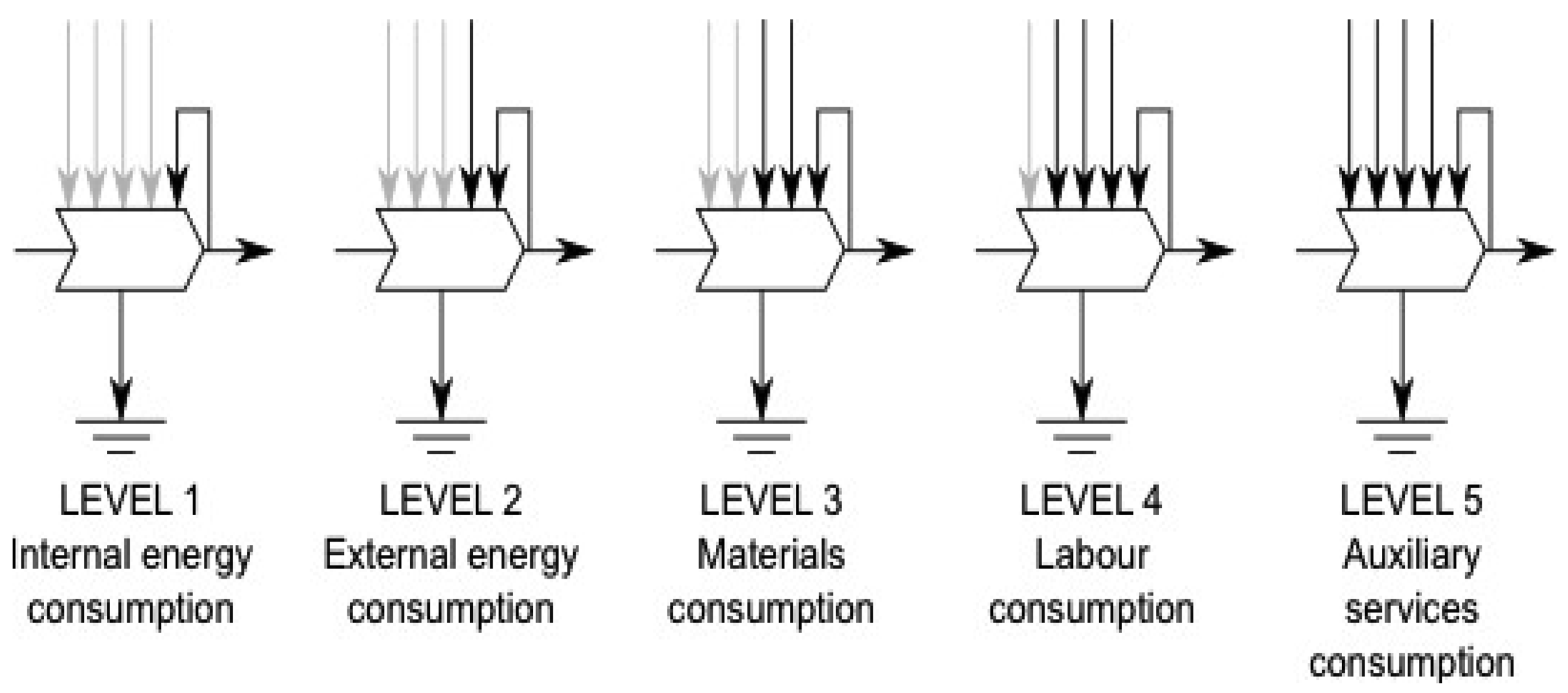
There are a number of dimensions along which a system boundary may vary. One dimension runs “parallel” to the energy process chain from extraction (‘mine-mouth’) to intermediate processing (“refinery gate”) to distribution (final demand) and determines the numerator in the EROI ratio, in answer to the question, “what do we count as energy outputs?” This dimension is depicted with the three system boundaries in Figure 1. Another dimension over which the system boundary may vary is to include a greater variety of direct and indirect energy and material inputs which determine the denominator of the EROI ratio, in answer to the question “what do we count as inputs?” This is illustrated in Figure 1. Level 1 includes only those inputs from the energy chain under investigation, level 2 incorporates energy inputs from the rest of the energy sector (this highlights the difference between the EROI, the internal and external energy ratios discussed in Section 5). Level 3 includes energy inputs embodied in materials, levels 4 and 5 incorporate energy embodied in supporting labor and other economic services.

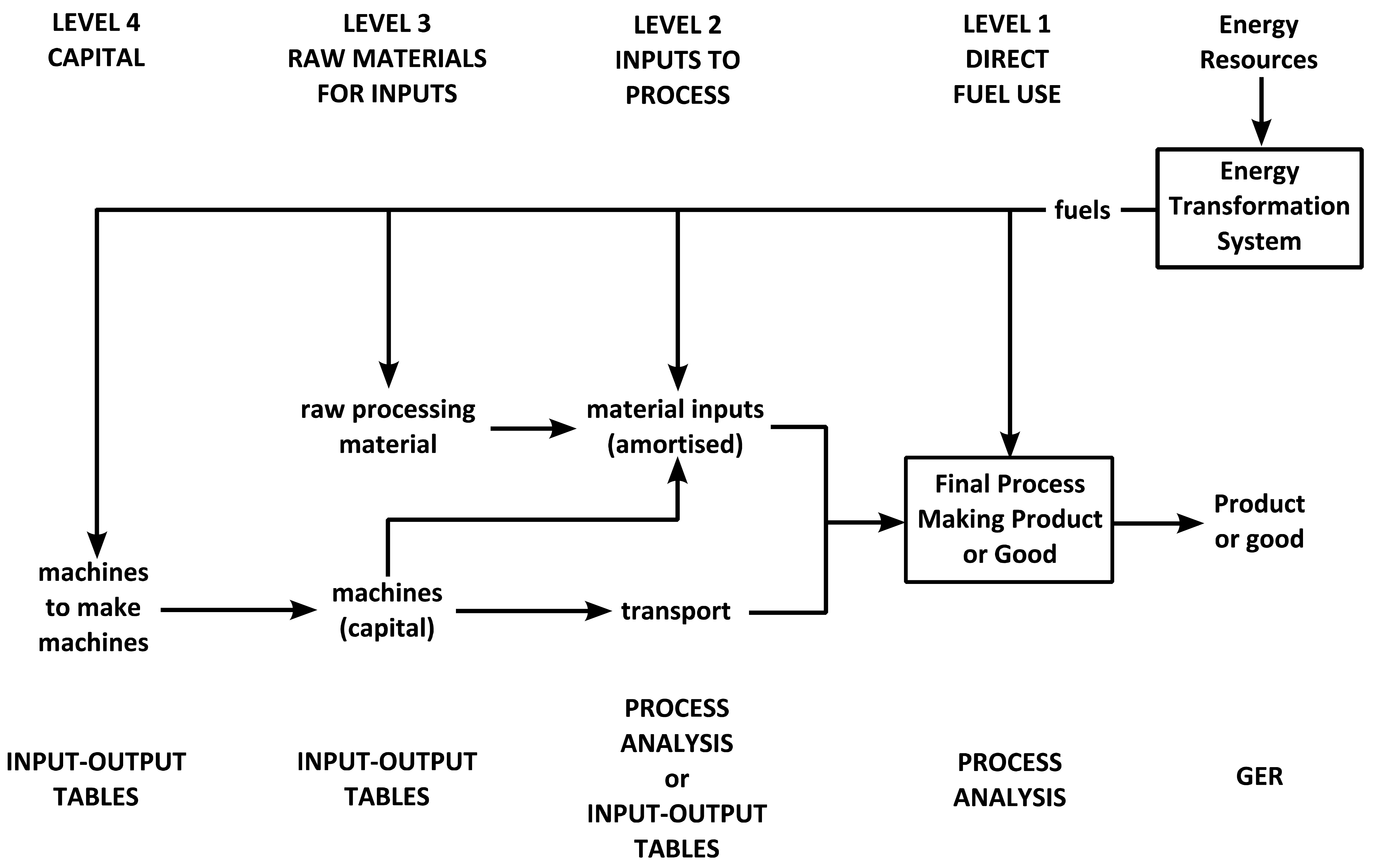
There are two main techniques within energy analysis to assess the energy flows through a particular process or product: (1) process analysis, or (2) economic input-output. Process analysis, also known as bottom-up analysis and akin to life-cycle analysis, accounts for the energy inputs and outputs in a process by aggregating them through the sequential stages of production. Economic input-output analysis, or top-down analysis, converts economic input-output tables into energy units by multiplying by sector-specific energy intensity values. A third method is emerging that is a hybrid of both of these methods. The choice of which method to use is normally made on the basis of where the system boundary is drawn (see Figure 1 and Figure 2), or by data restrictions.

For any production process, energy inputs may take a number of forms. Perhaps the most obvious is the energy used directly in the process itself, i.e., diesel fuel consumed on a drilling rig. But one may want to consider as well the energy that has been used to extract and deliver the material inputs to a process, such as the energy used to build the drilling rig. These machines involved in a process have also required energy for their manufacture, as have the machines that built those machines, and so on. We can differentiate amongst energy and material inputs as direct and indirect inputs, with numerous subdivisions within these broad classifications. For example, direct energy inputs consist of fuels used to run tractors for corn harvesting or natural gas used on a drilling platform, while indirect energy inputs would be the fuel used to run a farmer's car when he goes to get a part or to fly the laborers out to the drilling rig. Meanwhile, direct material inputs would be the embodied energy of the tractor or drilling rig, while indirect material inputs would be the embodied energy of the farmer's car or the helicopter.

Some components, such as labor, can be considered both direct and indirect energy inputs. Direct labor costs occur as muscle power used on the rig itself while indirect labor costs occur by the energy used to support the paychecks of the workers within steel mills that produce the steel to build the rig. Another category of inputs, external costs, or externalities, are costs imposed on society by the process under study but which are not reflected in the market price of the good or service. Burning diesel fuel to drill for oil releases sulfur and other greenhouse gas emissions into the atmosphere, a cost that is borne by society at large and one that is not accounted for when using the heat equivalent of the fuel as the only cost, and thus represents a limitation of EROI analysis. Emergy analysis is an attempt to include all energy inputs, including those from nature, with differential quality values (i.e., transformities) for each [17]. It is rarely used in energy analysis, but because of its comprehensive nature offers a useful upper limit to energy inputs.

Expanding the boundaries of an energy analysis tends to increase quickly the amount of data collection and analysis needed to calculate and energy ratio. In most cases, if the analyst is interested only in either direct fuel use or the direct material and transport inputs (as represented by levels 1 and 2), then process analysis may be used. If a higher level analysis is required, including material inputs for capital goods and the “machines to make the machines”, then input-output (I-O) tables will most likely prove more useful (Figure 3). A problem with that approach is that there has been essentially no good and reviewed work on the subject in the US for decades, with the possible exception of the unreviewed but easy to use numbers from the Green design Institute at Carnegie Mellon University, available on line.

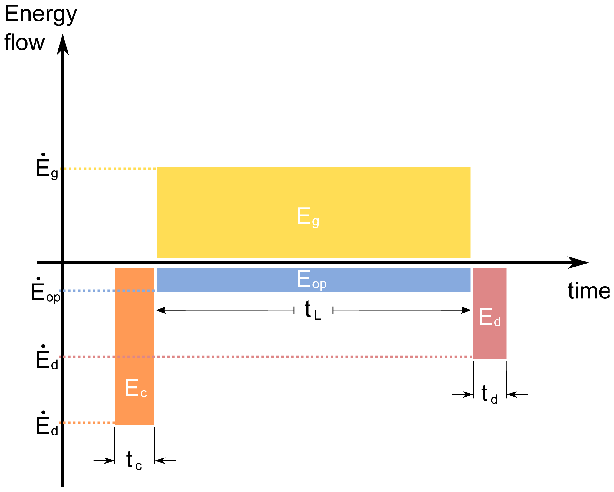
The system boundary may also vary along a temporal dimension. Figure 4 depicts an energy production project that begins at time t, with its construction, requiring a total energy input to construction of E_c. This energy is assumed to be used at a constant rate over the construction time, t_c, such that the energy flow to construction is:

$${\dot{E}}_c=E_c/t_c$$

Once the project starts producing energy it is assumed to produce a constant gross flow of energy at rate Ė_g over the whole lifetime t_L. An energy flow, Ė_op, is required to operate and maintain the project. At the end of the project lifetime, some energy, E_d is required for decommission [19]. The total net energy output from the plant over the whole lifetime is:

$$E_{\mathit{\text{net}}}=E_g-E_{op}-E_c-E_d$$

and the EROI is defined as:

$$\mathit{\text{EROI}}=\frac{E_g}{E_c+E_{op}+E_d}$$

(1)

When considering a system composed of many such plants with construction, operation and decommission staggered through time, such as the US oil industry, it becomes more difficult to define the lifetime over which energy inputs and outputs are being produced and invested. In such cases, the EROI is often defined such that,

$$\mathit{\text{EROI}}=\frac{{\dot{E}}_g}{{\dot{E}}_c+{\dot{E}}_{op}+{\dot{E}}_d}$$

(2)

This formulation of the EROI makes the assumption that investments and returns from those investments occur in essentially the same time period. This assumption would be accurate only if the system is in “steady state”, i.e., not growing or shrinking. It is important to note in this case that the EROI will be reduced in periods of heavy investment (such as happened during periods of high oil prices in the Seventies), which come to fruition only in subsequent years, during which time the EROI may be inflated.

2.1. A Two-Dimensional Framework for Choosing Boundaries in EROI Analysis

Establishing clear goals and objectives are the first steps in selecting the boundaries of an EROI analysis. For example, stating that the goal of a particular study is to “calculate the EROI of the production of corn ethanol, inclusive of on-farm and refinery costs,” gives the reader some perspective from the outset about the scale of the study being performed. Other studies may have similar objectives that require different boundaries. If the objective of another study was to “calculate the EROI of the production of corn ethanol inclusive of all costs incurred from the farm to the end-user”, the reader would realize that the boundaries of analysis for this study will be wider than the boundaries in the first study, and as a result, the EROI numbers calculated in these two studies should not be compared directly.

Once the objectives have been outlined, choosing the appropriate boundaries for an EROI analysis depends largely on two factors: (1) what level of energy inputs are going to be considered in the analysis (i.e., Figure 2), and (2) the methods chosen to aggregate energy units. Sometimes the data needed for analysis is defined in non-energy units (i.e., water in cubic meters). There are two methods for handling non-energy inputs in an EROI calculation. The first method, used most often, is to ignore (or simply list) non-energy inputs in the EROI analysis. The second is to convert the non-energy input into energy units using heat equivalents, or in emergy analysis, a weighting factor (called a transformity). When using heat equivalents for inputs and outputs, there are two options as well: nonquality-corrected and quality- corrected heat units. This difference arises from the idea that not all joules are created equal, and the economic utility of a unit of electricity is different from the utility of a unit of coal [20]. When aggregating heat units of different types of energy, a quality correction is often used to account for these differences. The various methods of accounting for quality differences in energy are discussed in the next section.

We can represent the information presented thus far in a simple, two-dimensional framework (

Table 1. Two-dimensional framework for EROI analysis. The system boundaries, which determine the energy produced from a process (i.e., the numerator of an EROI calculation) are across the top, while the boundaries that determine the energy inputs (i.e., the denominator of an EROI calculation) are listed down the left. The shaded cells represent those with boundaries that favor economic input-output analysis while the other cells favor process-based analysis.

Boundary for Energy Inputs		Boundary for Energy Outputs
		1. Extraction	2. Processing	3. End-Use
1	Direct energy and material inputs	EROI1,d	EROI2,d	EROI3,d
2	Indirect energy and material inputs	EROIstnd	EROI2,i	EROI3,i
3	Indirect labor consumption	EROI1,lab	EROI2,lab	EROI3,lab
4	Auxiliary services consumption	EROI1,aux	EROI2,aux	EROI3,aux
5	Environmental	EROI1,env	EROI2,env	EROI3,env

). The first row of Table 1 lists the system boundaries for energy outputs, i.e., the numerator of the EROI calculation. The boundary for the inputs is listed along the left side of the table. Thus it is possible to have a narrow boundary for the energy output, such as crude oil from an oil well, while using a very wide boundary for the energy inputs, such as the labor used to construct the steel to build the oil rig. Alternatively, one could use a very wide boundary for the energy outputs, such as the gasoline consumed by the end user, and a narrow boundary for the energy inputs, i.e., including only direct energy and material inputs at each stage in the production process.

The nomenclature suggested for EROI analyses follows logically from Figure 1. A researcher needs only to select the appropriate box for their specific research project and use the EROI tag associated with that box. For example, an EROI analysis that focuses on the extraction phase and includes simply the direct energy and material inputs would be deemed EROI_1,d. The “1” refers to the boundary for energy outputs in Table 1, while the “d” refers to the fact that only “direct” inputs are being considered. Since most EROI analyses account for both direct and indirect energy and material inputs, we have deemed this boundary to be the “standard EROI,” and assigned it the name EROI_stnd. Most often, the boundaries of an EROI analysis will be determined by the data available or the objectives, so it is advisable that the data be categorized into direct, indirect, etc. … so that the appropriate row in Table 1 can be chosen. We suggest that future EROI analyses include the calculation of EROI_stnd. If all EROI research includes this calculation in addition to any other EROI calculations, then we will have a basis by which to compare all energy resources. As a first step in this process, essentially all of the EROI calculations in the articles in this special issue have included calculations of EROI_stnd in addition to whatever other EROI calculations were performed. If both labor and environmental costs in addition to indirect costs are considered then you can write EROI_{1,i + lab + env} and so on. The important thing is to make what you include very clear.

2.2. An Example of Multiple Boundary EROI Analysis

Hall et al. [15] published a paper that calculated 3 different EROI values for the transportation system of the U.S., each EROI corresponding to standard, point of use, and “depreciation” [15]. EROI_stnd represents only the direct and indirect energy inputs and outputs from the oil extraction process up to the well-head. EROI_1,pou translates the same considerations to “point of use,” and this statistic includes direct energy inputs and outputs following the extraction (i.e. EROI_stnd), refining and transportation of fuel to the point of use, i.e., gas station. Thus EROI_pou represents and example of an EROI calculation that is specifically useful for this analysis, and would represent an additional row in Table 1 if it were added. EROI_ext is the widest boundary EROI calculated in Hall et al., and it represents all direct and indirect energy costs as well as the energy required to use that energy, including depreciation energy costs, such as the pro-rated maintenance of roads, bridges and automobiles that is necessary to maintain transportation networks to use that oil. EROI_ext would constitute another row in Table 1 if it were added. Since Hall et al. [15] chose to use the non-quality corrected energy units, all the EROI calculations are within the first column of Table 1.

3. Energy Quality

There are many different factors that determine the quality of a heat unit of fuel. We adopt the definition of energy quality proposed by Cleveland et al. [9]: the relative economic usefulness per heat equivalent unit of different fuels and electricity. Energy quality is determined by a complex set of attributes unique to each fuel such as physical scarcity, capacity to do useful work, energy density, cleanliness, amenability to storage, safety, flexibility of use, cost of conversion, and so on. One major criticism mounted against EROI research has been that it ignores many of these factors that determine the quality of an energy source. Converting all energy inputs to common energy units using only heat equivalents assumes implicitly that a joule of oil is of the same quality as a joule of coal or a joule of electricity. Since this is clearly not the case, we should account for differences of energy quality within EROI analysis when this is possible. Sometimes this can be done by incorporating the energy cost of upgrading the fuel to a given quality in the denominator while specifying the quality of the numerator.

There is uncertainty associated with all quality adjustments, as there is uncertainty with nearly any quantitative estimate outside the laboratory, but we believe the quality-adjusted energy units used in an EROI analysis are no better or worse on average than the numbers used in monetary cost-benefit analysis or other weighting procedures in economics.

Standard, non-quality corrected EROI calculations use thermal equivalents for all fuel sources to aggregate energy inputs:

$$E_t=E_{1t}+E_{2t}+\dots +E_{nt}$$

(3)

where E is an amount of energy of n types of energy sources in time period t. There are numerous methods to adjust for quality, and the following discussion of quality conversions is based on the options given in Cleveland (1992) and Cleveland (2000) [9,21].

3.1. Economic Methods to Adjust for Quality

Priced-based adjustment emerged from the literature as the method of choice when adjusting for energy quality. According to neoclassical economic theory, the price

$${\eta }_{nt}=\frac{P_{nt}}{P_{1t}}$$

per heat equivalent of fuel represents a myriad of factors that determine a fuel's utility, or quality, per heat unit. For these reasons the price per joule of electricity is greater than the price per joule of coal, i.e., electricity is more useful and therefore demands a premium price. The following equation calculates weights for each fuel type, n, for each time period t:

$$\text{EROI}={\dot{E}}_{\text{g}}/({\dot{E}}_c+{\dot{E}}_{\text{d}}+{\dot{E}}_{\text{op}})$$

(4)

where: η_nt is the weight assigned for energy type n in time period t, P_1t is the price of the reference fuel chosen at time t, and P_nt is the price of fuel n at time t. For example, if oil is chosen as the reference fuel, then the price per joule of electricity, coal, and all other energy types are divided by the price per joule of oil in time period t. Each weight is then multiplied by the amount of consumption of that fuel type during time period t to obtain the quality-adjusted energy input to the process.

$$E{\prime }_t={\eta }_{1t}{E}_{1t}+{\eta }_{2t}{E}_{2t}+\dots +{\eta }_{nt}{E}_{nt}$$

(5)

where E′ is the quality-adjusted energy aggregation and η is the weight of energy source η in time period t.

There are important assumptions with this method of quality adjustment. For example, using this type of price-based adjustment assumes that all fuels are perfectly substitutable [9]. As the price of one fuel increases relative to another, it can be replaced easily and fully. Although fuels are partial-substitutes, they are not perfectly substitutable, as is evident by the fact that energy users pay a premium for electricity and/or oil, more versatile energy sources, relative to coal, even though they can get the joule-equivalent energy in the form of coal for a cheaper price [22].

This method of comparing relative prices is sensitive also to rapid changes in the price of the reference fuel used. If one were using oil as a reference fuel, the doubling of the price of oil in 2008 would indicate that the quality of all other fuels decreased by half.

Yet if this same index were calculated using coal as the reference during the same period no such trend would appear across the whole index, except for the quality-weight for oil prices. Berndt (1978, 1990) suggests an adjusted form of the relative price approach that utilizes fuel shares as well as prices to weight the quality of each fuel type [22,23]. Berndt refers to this methodology as the “Divisia Index”, which is calculated according to the equation (repeated from [6]):

$$\ln E_t^{\prime }-\ln E_{t-1}^{\prime }=\sum _{n=1}^k\left(\right(\frac{P_{nt}{E}_{nt}}{2\text{∑}_{n=1}^k{P}_{nt}{E}_{nt}}+\frac{P_{nt-1}{E}_{nt-1}}{2\text{∑}_{n=1}^k{P}_{nt-1}{E}_{nt-1}})(\ln E_{nt}-\ln E_{nt-1}))$$

(6)

where p is the price of n different types of fuels and E is the final consumption of energy (joules) for each fuel type. This method allows for partial substitution amongst different fuel types and eliminates the over-dependence on a reference fuel type.

3.2. Shortcomings of Price-Based Adjustment

There are some shortcomings of a price-based weighting system. Many environmental and social costs are not incorporated into the market price for a fuel. These externalities cast doubt on the usefulness of using a price-based weighting system when comparing the sustainability of various extraction/production systems. But the problem of externalities can be ameliorated to some extent by including externalities in prices, such as through cap and trade programs for greenhouse gas emissions. Within this scenario, prices will increase as externalities are included and as this increase switches fuel shares to the low cost producer, the Divisia Index will shift as well.

Fundamentally, the fact that fuels have different prices per joule indicates that factors other than heat content are valued by energy consumers. Given the aforementioned shortcomings, prices produce quality weights for fuels that can be used to adjust energy data for differences in quality [20]. We suggest that EROI studies use either equation five or six to adjust energy data by the quality of fuel types, noting the assumptions and limitations of each method.

3.3. Quality Adjustments Using Physical Units

Exergy is a means by which one can account for quality differences between energy carriers using purely physical measures. It is defined as a measure of the ability of a system to perform work in the process of equilibrating with a reference state (normally chosen to be the atmosphere at standard temperature and pressure) [24]. As work is performed exergy is consumed until a point is reached at which the system under study has equilibrated with a reference state. Because a kilogram of oil can perform more work than a kilogram of coal because of its greater energy density, the exergy of oil is higher than that for coal (

Table 2. Specific exergy of different fuels, from Hermann [24].

Fuel	Exergy [MJ/kg]	Error (+/−)
Coal	25.00	5.00
Bituminous coal (Blacksville)	29.81
Bituminous coal (Absaloka)	19.87
Petroleum	42.00	2.00
Heavy oil (bitumen)	40.00
Oil shale (Estonian)	12.00
Tar sands (US)	6.00
Natural gas (representative, 80% humidity)	50.50
Methane clathrate (Mid-America trench)	4.80
Uranium 235	75000000.00
Uranium 238	77000000.00
Thorium 232	78000000.00
Lignin	25.00
Cellulose	17.00	1.00
Eucalyptus (dry)	19.90
Poplar (dry)	19.20
Corn stover (dry)	18.20
Bagasse (dry)	17.80
Water hyacinth (dry)	15.20
Brown kelp (dry)	10.90
OTEC (20K difference)	<0.01
Geothermal (150K difference)	0.13

). In this way, exergy provides a method to quality-correct energy carriers based on physical units. It should be mentioned that, although both exergy and prices can be used to adjust for quality differences in energy carriers, they are different metrics. That is, prices are based on differences in density, transportability, etc., whereas exergy is based only on differences in the ability to do work [6].

Whereas total energy is conserved in every process, exergy is not. Exergy consumption is proportional to entropy creation [25]. The exergy, E, of a system A in an infinite (i.e., unchangeable) environment A₀, is defined as:

$$E=U+P_{0}V-T_{0}S-\sum _i{\mu }_{i0}{n}_i$$

Where U, V, S and n_i are respectively the internal energy, volume, entropy and number of moles of material type i of system A. P₀, T₀ and μ_i0 are the pressure, temperature and potentials (e.g., chemical, nuclear, gravitational, etc.)[26] of material type i for the environment A₀. U is calculated using the Gibb's relation:

$$U=ST-VP+\sum _i{n}_i{\mu }_i$$

Substituting, we find a new formulation for the exergy of system A₀:

$$E=S(T-T_0)-V(P-P_0)+\sum _i{n}_i({\mu }_i-{\mu }_{i0})$$

From this formulation we can see that once system A has equilibrated with the environment A₀ (i.e., T − T₀ = P − P₀ = μ_i − μ_i0 = 0) then the exergy of system A is zero. In other words, all of the exergy has been consumed, and no further work can be accomplished.

3.4. Shortcomings of Exergy-Based Adjustments

Exergy is an attractive approach to adjusting energy data for differences in quality since it avoids using economic data, such as prices, and the problems associated with them (e.g., inflation). However, exergy cannot capture many properties of a fuel or energy carrier that contribute to its economic attractiveness, such as transportability, global warming potential, toxicity, or cleanliness [9]. Exergy analyses also ignore important critical inputs such as capital and labor [27]. Economic methods may be able to capture such characteristics.

4. Deriving Energy Intensities from Economic Data

Often, the only data available, or available for free, for capital equipment and other energy or material inputs is economic data. Because of this, there is often a need to convert dollars to energy units. The most straightforward method is to use an energy intensity value, i.e., a value reported in units of energy per dollar (ex. joules per dollar). Which energy intensity value should be used is a more difficult question to answer.

Dividing energy consumption by dollar output for a given economy and time period yields an average energy intensity value that can then be used to convert other monetary information to energy units. This average energy intensity is a measure of the output, measured in dollars (or other currency), created from a given amount of energy input to the economy or process. Although useful for quick calculations, the basic national-level energy intensity value is a coarse measurement, as it averages values across sectors of the economy that are quite different. The average energy intensity for the U.S. economy in 2005 was 8.3 MJ/$ (Table 2). We provide other data (mostly based on heat equivalents per ton) from 2005 in

Table 3. Various conversions used commonly in EROI analysis.

Unit	Conversion Factor	Reference
Primary Energy (Heat Content)
Oil	6.12 (GJ/bbl)	[31]
Natural Gas	41 (KJ/m3)	[31]
Coal	22 (GJ/tonne)a	[31]
Energy Intensities (for year 2005)	MJ/$
average U.S. economy	8.3	[15]
average heavy industry	14	[15]
average oil & gas exploration and dev.	20	[12]
Material Costs	GJ/tonne
Aluminum	241.2	[32]
	100.2	[33]
	272.2	[34]
	11.7b–140	[35]
Steel	32.4	[32]
	9.43c–25.2d	[35]
Copper	200.2	[33]
	93.7	[36]
	104.4	[37]
	51.7–179.7	[38]
	0.08–255.7	[39]
Cement	5.5	[34]
Iron Ore	0.34–2.9	[39]
Stone	0.021–0.057	[39]
Limestone	0.034	[39]
Lead	1.4–31.1	[39]
Zinc	76	[39]
Phosphate	0.083–0.349	[39]
Glass
Molten Flint Glass	14.2	[35]
Molten Emerald Glass	11.7	[35]
Molten Amber Glass	13.2	[35]
Plastics
Polyvinyl Chloride (PVC)	59.8	[35]
General Purpose Polystrene (GPPS)	84.8	[35]
High Density Polyethylene (HDPE)	89.5	[35]
High Impact Polystyrene (HIPS)	87.4	[35]
Low Density Polyethylene (LDPE)	93.9	[35]
Polyethyene Terephthalate (PET)	88.9	[35]
Polypropylene (PP)	88.5	[35]
Linear Low Density Polyethylene (LLDPE)	83.4	[35]
Woode
Dry Lumber	2.33	[35]
Green Lumber	0.95	[35]

^aAverage U.S. coal production;^bsecondary aluminum ingot;^cElectronic Arc Furnace Billet;^dHot Rolled Coil (Integrated Mill);^eAverage of hardwood and softwood.

Oil and gas production are energy-intensive sectors of the economy as is general industrial production (e.g., of drill bits, pipes and so on). Bullard and Henrendeen (1975) and Costanza (1980) recognized the shortcomings of using mean national energy intensity values and instead derived very explicit industry-specific values using Leontief type input-output (I-O) tables and industry-specific energy intensities to calculate sector-specific energy intensity values for the U.S. economy [28,29]. An inflation- corrected value for heavy industries derived from earlier work by Bullard, Hannon and Herendeen (about 16,000 Kcal per dollar in 1972), is 14.3 MJ/dollar in 2005 when corrected for units and inflation with the Consumer Price Index (CPI).

These data are very comprehensive but very old. Herendeen (pers. comm.) suggested in 2005 that while far from perfect one can use the more recent I-O energy intensities derived from the Carnegie Mellon web site for a general upstream average for inputs to the energy sector [30]. There are sometimes disquieting differences from one category to another, but they are the best we have now. One derives from their “model” a value of 14.5 MJ energy used per dollar spent for “oil and gas extraction” in 2002. This value is about half way between the energy intensities for the entire economy (8.3 MJ per 2005 dollar) and for money spent by the US and the UK by the entire oil and gas exploration and development industry, including the money spent directly on energy itself. Gagnon et al. (2009) estimated that the energy intensity for oil and gas exploration was 20 MJ/dollar in 2008 [12]. Thus we use an energy intensity for industrial activity (i.e., for things purchased by energy companies) of 14 MJ/dollar in 2005. That value for another nearby year can be derived using the consumer price index. When we used oil-industry specific correctors some were higher and some lower than the CPI, so we did not feel that anything was gained from using other inflation-adjusters than the CPI.

The specific energy intensity values used in an EROI analysis should match the general level of precision of the EROI analysis being performed. For example, if one is calculating the EROI of exploration and development within the oil and gas sector, and the only exploration data obtainable is the dollar cost of building a drilling platform, then an energy intensity value calculated for heavy industry, or optimally for oil and gas exploration in that country, should be used. The best option is to get direct energy and material use estimates and hence avoid the use of energy-intensity values altogether, but this is rarely possible. In most cases, we believe that omitting data because it uses dollars instead of energy units creates more error than including that data via an energy intensity conversion. Many of the papers in this special issue explore uncertainties associated with these values through sensitivity analysis.

5. Alternative EROI Statistics

5.1. Fossil Energy Ratio

The widespread application of net energy analysis to different fields of science has led to the creation of numerous variants of the conventional EROI statistic (now referred to as EROI_stnd) [40]. Two variants in particular seem to garner the most attention within the literature. The first alterative EROI statistic is called “Fossil Energy Ratio” (FER), which compares the total energy gains from fossil fuel investment only. FER is used often in the discourse on biofuels; much of the energy inputs to biofuel production are technically renewable, such as burning biomass during the production of corn ethanol, so FERs tend to be much higher than EROIs for biofuels [41].

5.2. External Energy Ratio

The second alternative EROI statistic is called “External Energy Ratio” (EER). EER is a useful measure for energy production techniques that consume a significant amount of energy derived in situ. For example, one method of tar sand production burns a portion of the bitumen in situ as a means to heat and crack the surrounding bitumen so that it will flow more easily. Since the heat energy derived from the bitumen originates within the extraction process, it is excluded from an EER calculation, although it would be included within a conventional EROI calculation. EER is calculated as:

$$\text{EER}={\text{O}}_{\text{d}}{/\text{I}}_{\text{d}}{+\text{I}}_{\text{emb}}{+\text{I}}_1$$

Both FER and EER are more restricted forms of the standard EROI calculation. By definition both FER and EER must be greater than or equal to the standard EROI for the same system, since FER and EER use a sub-sample of the total energy inputs to a process, yet include the same energy output.

5.3. Net Energy Yield Ratio

The net energy yield ratio (NEYR) has as the numerator the net energy from the energy production process and all of the inputs necessary to produce that net flow as the denominator:

$$\mathit{\text{NEYR}}=\frac{O_d-I_d-I_{\mathit{\text{rec}}}-I_{\mathit{\text{emb}}}-I_{\mathit{\text{lab}}}}{I_d+I_{\mathit{\text{rec}}}+I_{\mathit{\text{emb}}}+I_{\mathit{\text{lab}}}}$$

5.4. Absolute Energy Ratio

The absolute energy ratio (AER) includes in the denominator the energy content of the energy resource from the natural environment, I₀, which is being processed [19]. As such the AER must be less than unity. It may be considered a “life-cycle” efficiency:

$$\mathit{\text{AER}}=\frac{O_d}{I_0+I_d+I_{\mathit{\text{rec}}}+I_{\mathit{\text{emb}}}+I_{\mathit{\text{lab}}}}$$

6. Step by Step Instructions for EROI Analysis

The objective of this section is to combine the different aspects of EROI analysis presented in sections one through five into a short, unambiguous procedure for conducting an EROI analysis.

Step 1. State objectives

The first step in performing an EROI analysis is to state the objectives of the analysis clearly. This will allow the reader to get a sense of the scale of analysis being performed and whether or not there are other analyses with similar objectives.

Step 2. Create a flow diagram and identify system boundaries

Figure 1 represents a generic flow diagram for any system, and can be used as a reference. The symbolism developed by Odum (1983) and Hall and Day (1977) for systems flow diagrams is recommended when drawing the flow diagram for an EROI analysis [42,43]. All direct indirect, and embodied energy inputs and outputs should be included in this flow diagram.

Step 3. Identify all appropriate inputs and outputs within system boundaries

Once the flow diagram is complete, the various flows of energy, defined by arrows connecting two symbols, should be identified and labeled on the flow diagram as either direct, indirect, or embodied energy inputs or outputs. We recommend using the concepts and nomenclature developed in Figure 1 as a base.

Step 4. Indentify data needed for the calculation of EROIstnd as well as any other EROI calculations

Once steps one through three are completed, the analyst should have sufficient knowledge to identify which specific EROI calculation is being performed as, or in addition to, EROI_stnd. At this point the analyst should identify the specific EROI calculations that they are performing by using the labels provided in Table 1 and define the EROI equation by placing the appropriate energy flows from the flow diagram developed in step 1 into the numerator and denominator of the EROI calculation.

Step 5. Choose method of energy quality adjustment

All of the energy inputs and outputs should be undertaken with both heat equivalents and quality-adjusted energy if possible. We recommend using a price-based aggregation or a Divisia approach for quality adjustments, as outlined in Section 3, unless there is a good reason for doing otherwise. At a minimum, electricity should be multiplied by a factor of 2.6 to represent mean thermal requirements. The analyst should spend time identifying the benefits and shortcomings associated with whichever method is chosen, including any underlying assumptions. For example, if an EROI analysis uses mainly one energy type for inputs and outputs, then a quality adjustment adds little value. For most EROI analyses, a basic price-based adjustment is adequate.

Step 6. Identify and convert financial flows

Often times only financial data is available for energy flows, such as the cost of transporting oil. This data needs to be converted to energy units using an energy intensity value. Section 4 can be referenced for a full discussion of how to derive energy intensity values and which intensities are appropriate for various analyses. Once these financial flows are identified, convert them to energy units using whichever energy intensity value was chosen.

Step 7. Calculate EROI

This is the final step in the process where all of the energy units are aggregated and the EROI value is calculated. Each EROI analysis should have at a minimum the EROI_stnd as well as any other EROI calculations of interest. The investigator can then compare his or her EROI_stnd with others, and indicate whether and how an alternate EROI adds useful information.

7. Further Issues

A number of issues remain that have not been discussed in the preceding analysis. These are concerned with: (1) accounting for non-energy inputs or impacts; (2) access to data; (3) allocation of costs between co-products.

7.1. Accounting for Non-Energy Inputs and Impacts

It should be noted that although EROI analysis is useful because it provides a single statistic by which multiple energy options can be compared, it is limited in that all inputs and outputs must be converted to energy units. Often there are inputs or outputs from a process that are valuable for reasons other than their energetic value. Water for irrigation is a good example. Although we can calculate the energy cost of irrigation, this does not account for water's role in photosynthesis or the relative scarcity, pollution or depletion of water in an aquifer. In addition, “outputs” from energy production such as pollution (externalities in economic terms) are difficult to capture in energy terms. These types of issues are of current interest in EROI research, but until a consensus emerges as to how to handle non-energy inputs and outputs, energy equivalents should be used. Each researcher should note any of these types of important methodological assumptions within their study.

7.2. Access to Data

When studying real world systems, there is always a trade-off between the costs involved and the benefit accrued in obtaining more data. Much of the data needed for energy analysis is not kept by the organizations running the processes involved. In many cases this speaks to the need to convert economic to energy data (as discussed in Section 4). There now exist many LCA databases (such as Gabi or SimaPro) storing information on energy inputs to various materials. As these kinds of analyses become more widespread, this information will become available.

7.3. Allocation Between Co-Products

Many production processes produce more than one type of good. A good example is an oil refinery that produces many chemicals, e.g., lubricants, as well as various grades of fuel. How should the costs of production be allocated between these different goods? Three options present themselves immediately: allocation by mass, allocation by energy content (either heating value, exergetic or divisia weighted), or allocation by price. The division of costs will be different in each case and it is unclear that one method is clearly “better” than any other. This issue is discussed extensively within the LCA literature (e.g., Reap et al., 2008 and Curran, 2007) [44,45].

In conclusion we believe that if these protocols are followed (including our provisions for flexibility) that EROI can rightfully take its place as a very powerful tool for evaluating some very important aspects of the utility of different fuels, and for helping to understand the implications of EROI changes for our economy as partly outlined in the introduction to this special issue. Most importantly good EROI analysis can save us from investing large amounts of our remaining fossil fuels into alternative fuels that contribute little or nothing to our nation's financial or energy well being, as appears to have been the case with corn-based ethanol and is likely to be the case with many energy alternatives that are being promoted by various interests.

References and Notes

- Lynch, M.C. Forecasting oil supply: Theory and practice. Q. Rev. Econ. Finance 2002, 42, 373–389. [Google Scholar]
- Radetzki, M. Peak Oil and other threatening peaks-Chimeras without substance. Energy Policy 2010, 38, 6566–6569. [Google Scholar]
- Campbell, C. Why dawn may be breaking for the second half of the age of oil. First Break 2009, 27, 53–62. [Google Scholar]
- Campbell, C.J.; Laherrere, J.H. The End of Cheap Oil. Sci. Am. 1998, 278, 78–83. [Google Scholar]
- Farrell, A.E.; Plevin, R.J.; Turner, B.T.; Jones, A.D.; O'Hare, M.; Kammen, D.M. Ethanol can contribute to energy and environmental goals. Science 2006, 311, 506–508. [Google Scholar]
- Cleveland, C. Net energy from the extraction of oil and gas in the United States. Energy 2005, 30, 769–782. [Google Scholar]
- Murphy, D.J.; Hall, C.A.S.; Powers, B. New perspectives on the energy return on (Energy) investment (EROI) of corn ethanol. Eviron. Dev. Sustainability 2010, 13, 179–202. [Google Scholar]
- Hammerschlag, R. Ethanol's energy return on investment: A survey of the literature 1990–present. Environ. Sci. Technol. 2006, 40, 1744–1750. [Google Scholar]
- Cleveland, C.J.; Kaufmann, R.K.; Stern, D.I. Aggregation and the role of energy in the economy. Ecol. Econ. 2000, 32, 301–317. [Google Scholar]
- Murphy, D.J.; Hall, C.A.S. Year in review-EROI or energy return on (Energy) invested. Ann. N. Y. Acad. Sci. 2010, 1185, 102–118. [Google Scholar]
- Guilford, M.C.; Hall, C.A.S.; O'Connor, P.; Cleveland, C.J. A new long term assessment of energy return on investment (EROI) for U.S. oil and gas discovery and production. Sustainability 2011, 3, 1866–1887. [Google Scholar]
- Gagnon, N.; Hall, C.A.S.; Brinker, L. A preliminary investigation of the energy return on energy invested for global oil and gas extraction. Energies 2009, 2, 490–503. [Google Scholar]
- Mulder, K.; Hagens, N.J. Energy return on investment: Towards a consistent framework. Ambio 2008, 37, 74–79. [Google Scholar]
- Environmental Management-Life Cycle Assessment-Principles and Framework; ISO 14040:1997. ISO Copyright Office: Geneva, Switzerland, 1997. Available online: http://www.iso.org/iso/catalogue_detail.htm?csnumber=23151 (accessed on 8 December 2010).
- Hall, C.A.; Balogh, S.; Murphy, D.J. What is the minimum EROI that a sustainable society must have? Energies 2009, 2, 1–25. [Google Scholar]
- Hall, C.A.S.; Kaufmann, R.; Cleveland, C.J. Energy and Resource Quality: The Ecology of the Economic Process; John Wiley and Sons: Hoboken, NJ, USA, 1986. [Google Scholar]
- Odum, H.T. Self-organization, transformity, and information. Science 1988, 242, 1132–1139. [Google Scholar]
- Peet, J.; Baines, J. Energy Analysis: A Review of Theory and Applications; NZERDC: Report No. 126; Auckland, Australia, 1986. [Google Scholar]
- Herendeen, R.A. Net energy analysis: Concepts and methods. In Encyclopedia of Energy.; Elsevier: New York, NY, USA, 2004; Volume 4, pp. 283–289. [Google Scholar]
- Kaufmann, R.K. The relation between marginal product and price in U.S. energy markets. Energy Econ. 1994, 16, 145–158. [Google Scholar]
- Cleveland, C.J. Energy quality and energy surplus in the extraction of fossil fuels in the U.S. Ecol. Econ. 1992, 6, 139–162. [Google Scholar]
- Berndt, E.R. Aggregate energy, efficiency and productivity measurement. Annu. Rev. Energy 1978, 3, 225–273. [Google Scholar]
- Berndt, E.R. Energy use, technical progress and productivity growth: A survey of economic issues. J. Prod. Anal. 1990, 2, 67–83. [Google Scholar]
- Hermann, W.A. Quantifying global exergy resources. Energy 2006, 31, 1685–1702. [Google Scholar]
- Rosen, M.A. Exergy analysis of energy systems. In Encyclopedia of Energy; Elsevier: New York, NY, USA, 2004; Volume 2, pp. 607–621. [Google Scholar]
- Exergy, Wall, G. According to Wall the potential, μ, is a means by which to include properties of a material which affect the internal energy, U, but which are not included in the classical thermodynamic state variables, for example, gravitational potential energy due to altitude. Encyclopedia of Energy; Cutler, J.C., Ed.; Elsevier: New York, NY, USA, 2008. Available online: http://www.eoearth.org/article/Exergy (accessed on 17 October 2011). [Google Scholar]
- Hau, J.L.; Bakshi, B.R. expanding exergy analysis to account for ecosystem products and services. Environ. Sci. Technol. 2004, 38, 3768–3777. [Google Scholar]
- Bullard, C.; Herendeen, R. The energy costs of goods and services. Energy Policy 1975, 3, 279–284. [Google Scholar]
- Costanza, R. Embodied energy and economic valuation. Science 1980, 210, 1219–1224. [Google Scholar]
- Economic Input-Output Life Cycle Assesment. Carnegie-Mellon: Pittsburg, Pennsylvania, 2009. Available online: http://www.eiolca.net/cgi-bin/dft/use.pl (accessed on 8 December 2010).
- EIA. Annual Energy Review 2009; DOE/EIA-0384; U.S. Department of Energy: Washington, DC, USA, 2010. [Google Scholar]
- Demkin, J.A. Environmental Reserouce Guide; John Wiley and Sons: Hoboken, NJ, USA, 1996. [Google Scholar]
- Ruth, M. Thermodynamic constraints on optimal depletion of copper and aluminum in the United States: A dynamic model of substitution and technical change. Ecol. Econ. 1995, 15, 197–213. [Google Scholar]
- Energy Use, Loss and Opporutnities Analysis: U.S. Manufacturing and Mining; U.S. Department of Energy: Washington, DC, USA, 2004.
- Canadian Raw Materials Database. University of Waterloo: Waterloo, ON, Canada, 2010. Available online: http://crmd.uwaterloo.ca/index.html (accessed on 8 December 2010).
- Castle, J.F. Energy Consumption and Costs of Smelting; IMM Institute of Mining and Metallurgy: London, UK, 1989. [Google Scholar]
- An Assesment of Energy Requirements in Proven and New Copper Processes; U.S. Department of Energy: Washington, DC, USA, 1980.
- Herendeen, R. University of Illinois: Edelstein, IL, USA, Personal Communication; 2010.
- BCS. Mining Industry of the Future: Energy and Evnironmental Profile of the U.S. Mining Industry; U.S. Department of Energy: Washington, DC, USA, 2002. [Google Scholar]
- Spitzley, D.V.; Keoleian, G.A. Life Cycle Environmental and Economic Assessment of Willow Biomass Electricity: A Comparison with Other Renewable and Non-Renewable Sources; University of Michigan-Center for Sustainable Systems: Dearborn, MI, USA, 2005. [Google Scholar]
- Shapouri, H.; Duffield, J.A.; McAloon, A.; Wang, M. The 2001 Net Energy Balance of Corn-Ethanol. Proceedings of the Corn Utilization and Technology Conference, Indianapolis, IN, USA, 7–9 June 2004.
- Hall, C.A.S.; Day, J.J.W. Ecosystem Modeling in Theory and Practice; University Press of Colorado: Boulder, CO, USA, 1977. [Google Scholar]
- Odum, H.T. Systems Ecology: An Introduction; John Wiley and Sons: Hoboken, NJ, USA, 1983. [Google Scholar]
- Reap, J.; Roman, F.; Duncan, S.; Bras, B. A survey of unresolved problems in life cycle assessment. Int. J. Life Cycle Ass. 2008, 13, 374–388. [Google Scholar]
- Curran, M. Studying the effect on system preference by varying coproduct allocation in creating life-cycle inventory. Environ. Sci. Technol. 2007, 41, 7145–7151. [Google Scholar]
© 2011 by the authors; licensee MDPI, Basel, Switzerland. This article is an open access article distributed under the terms and conditions of the Creative Commons Attribution license (http://creativecommons.org/licenses/by/3.0/).
Share and Cite
Murphy, D.J.; Hall, C.A.S.; Dale, M.; Cleveland, C. Order from Chaos: A Preliminary Protocol for Determining the EROI of Fuels. Sustainability 2011, 3, 1888-1907. https://doi.org/10.3390/su3101888
Murphy DJ, Hall CAS, Dale M, Cleveland C. Order from Chaos: A Preliminary Protocol for Determining the EROI of Fuels. Sustainability. 2011; 3(10):1888-1907. https://doi.org/10.3390/su3101888
Chicago/Turabian StyleMurphy, David J., Charles A.S. Hall, Michael Dale, and Cutler Cleveland. 2011. "Order from Chaos: A Preliminary Protocol for Determining the EROI of Fuels" Sustainability 3, no. 10: 1888-1907. https://doi.org/10.3390/su3101888