A Dynamic Function for Energy Return on Investment


Abstract
: Most estimates of energy-return-on-investment (EROI) are “static”. They determine the amount of energy produced by a particular energy technology at a particular location at a particular time. Some “dynamic” estimates are also made that track the changes in EROI of a particular resource over time. Such approaches are “bottom-up”. This paper presents a conceptual framework for a “top-down” dynamic function for the EROI of an energy resource. This function is constructed from fundamental theoretical considerations of energy technology development and resource depletion. Some empirical evidence is given as corroboration of the shape of the function components.1. Introduction
Energy is fundamentally important to all of the processes that occur within our modern, (post)industrial society. It has been famously described by James Clerk-Maxwell as, “the ‘go’ of things” [1]. Modern society currently uses around 500 exajoules (1 EJ = 1018 J) of primary energy, 85% of which comes from fossil fuels. Some proportion of this 500 EJ must be used in the extraction and processing of energy resources, as well as in the manufacture of energy technology infrastructure, such as oil rigs and dams for hydroelectricity. This paper is intended as a discussion piece regarding some of the conceptual issues surrounding long-term dynamics of the energy supply system which may be understood using the dynamic EROI function.
1.1. Energy Analysis
Energy analysis is the process of measuring the energy flows through the process or system under investigation. According to Boustead and Hancock [2], “Energy analysis is a technique for examining the way in which energy sources are harnessed to perform useful functions” Peet [3] classifies energy analysis as, “determination of the amount of primary energy, direct and indirect. that is dissipated in producing a good or service and delivering it to the market” reflecting the current focus of energy analyses on economic activities. Energy analysis is important for a number of reasons:
firstly, because of the adverse environmental impacts linked with energy transformation processes, especially of concern recently being the emission of greenhouse gases associated with the combustion of fossil fuels (possible solutions include carbon capture and storage (CCS), however the increased energy consumption entailed by CCS may (dis)favor certain methods of energy production);
secondly, because of the finite availability of fuels and other energy resources (whereas non-renewable resources are finite in terms of total quantity, renewable resources are finite in the magnitude of their flow) and;
thirdly, because of the strong link between net energy and the material standard of living and economic opportunity offered by a society [4].
There is evidence that the qualities (i.e., net energy returns) of the major energy sources in use by society (coal, oil and gas) are declining [5]. Ceteris paribus, a decline in EROI of energy resources will increase the environmental impacts of an energy production process. Also, since more energy must be extracted to deliver the same amount of net energy to society this will entail faster consumption of finite energy resources. A society dependent on energy resources with lower EROI must also commit relatively more energy to the process of harnessing energy, hence has less available for other economic activities.
1.1.1. Net Energy and EROI
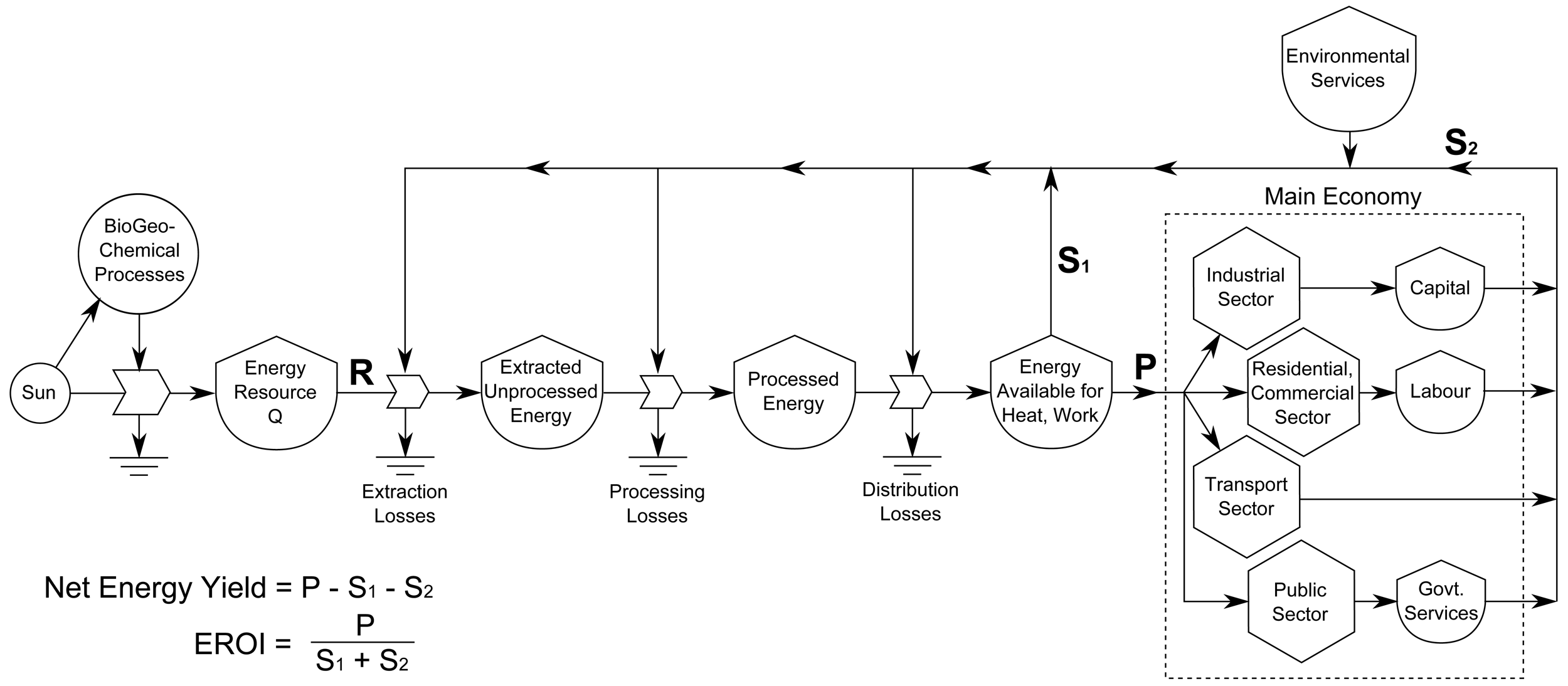
Whereas standard econometric energy models, such as MESSAGE [6], MARKAL [7] and the IEA's WEM [8], account only for gross production by the energy sector, P, net energy analysis (NEA) considers all energy flows between the energy sector and the rest of the economy, as depicted in Figure 1. The energy sector receives two inputs from the rest of the economy in order to produce energy. Inputs in the form of energy, S1 enable the energy sector to run its equipment, i.e., process energy. Inputs in the form of human-made-capital (HMC), S2, are the physical plant that must be put in place in order to extract energy from the environment, e.g., oil wells, wind turbines, hydro dams, etc.
In order to determine the net energy yield or benefit (the gross energy production less energy needs for extraction and processing), P − (S1 + S2), the ratio of energy produced to the energy needed to obtain this yield, P/(S1 + S2) is known as the net energy ratio (NER) or energy-return-on-investment (EROI) [9].
A reduction in net energy yield may occur for one of three reasons:
the energy flow rate of the resource is declining, such as due to an increase in the water production of an oil field;
more energy is required to extract the resource, such as oil extraction by pumping down steam or gas during enhanced oil recovery (EOR) or;
both 1 and 2 are occurring simultaneously.
In all cases the amount of energy required to produce a unit of energy output increases. This greater energy requirement will either be made up by utilizing energy flows from within the same energy production process (internal), such as an oil producer using oil from the field to produce steam for EOR, or from energy flows originating outside of the process (external), such as an oil producer using coal or natural gas for the same purpose [10]. In the latter case, the oil production process may be competing directly with other end-uses for the energy. Many authors have begun questioning the effects that declining EROI values will have on the economy [3–5,11,12].
2. A Dynamic Function for EROI
2.1. Theoretical Considerations
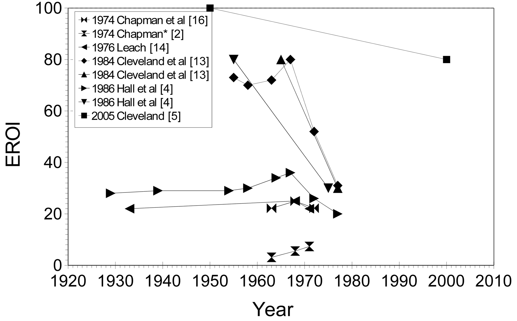
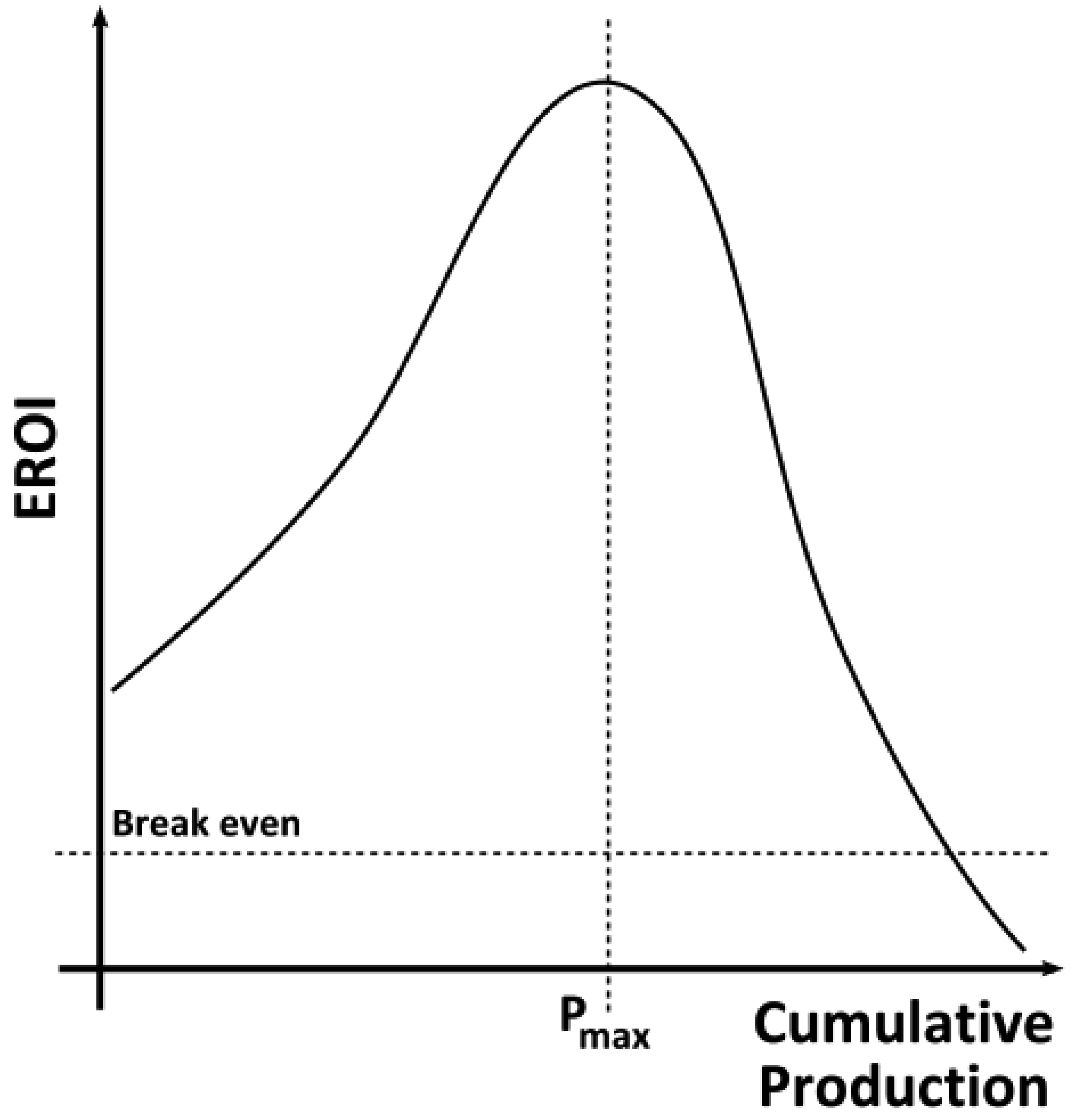
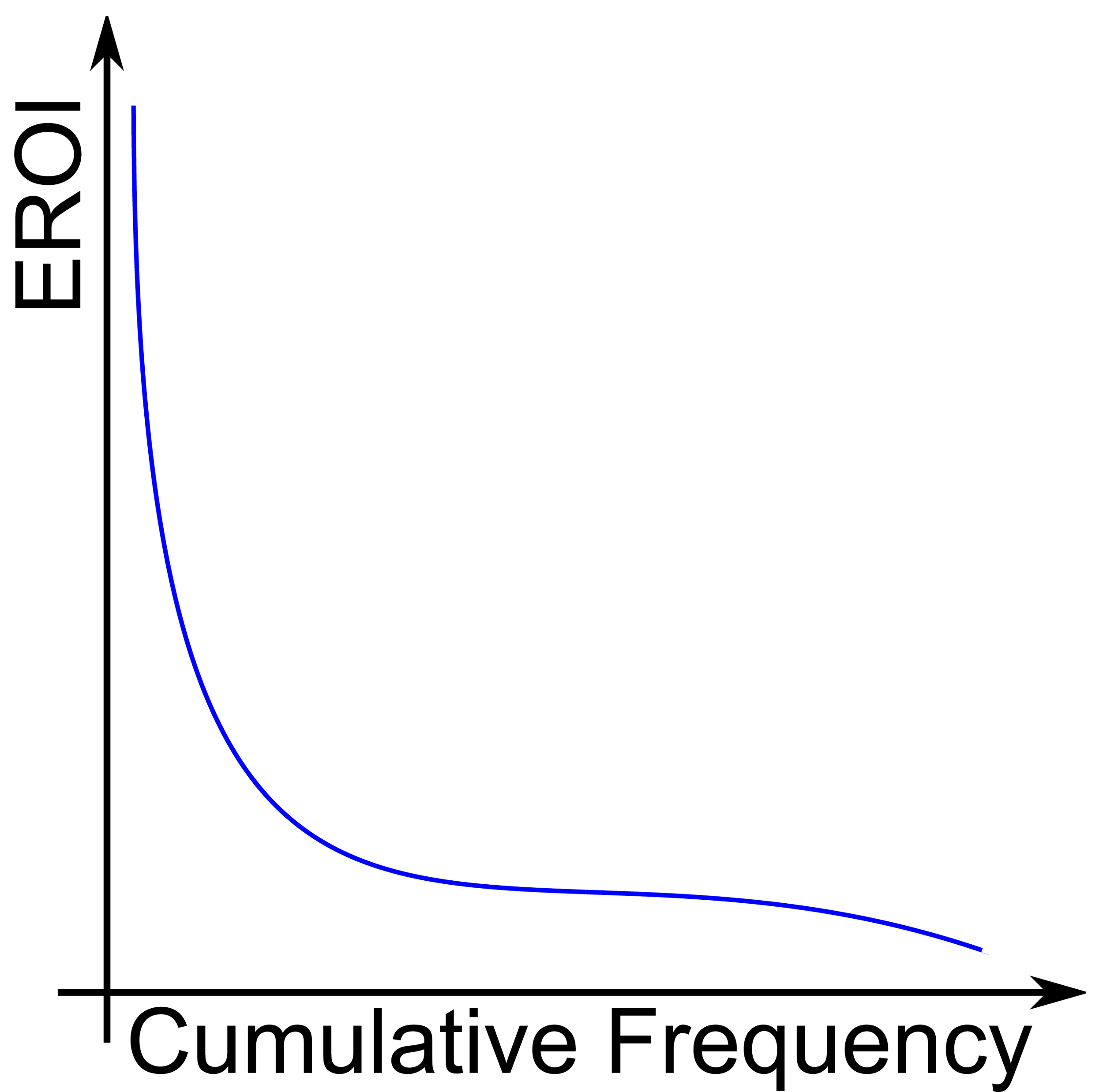
Most estimates of EROI are made as static estimates of a resource at a particular moment in time. The authors have located over 500 such estimates for all of the energy resources currently under development, as well as some still under R & D. Some dynamic estimates have been made which track the EROI of a particular fossil resource as it changes over time. A number of such studies track the EROI of coal and oil production from various different resources over several decades [4,5,13–16], as depicted in Figures 2 and 3. The studies show that the EROI of most energy resources (coal and oil) has been either (relatively) stable at an EROI of 20–40 or decreasing over time, some from an EROI of over 100. One such study has been conducted by Costanza and Cleveland [17] of oil and gas production in Louisiana. They identify a very characteristic shape for the EROI as a function of cumulative production, as shown in Figure 4. The EROI of the resource initially increases before reaching some point of production, Pmax, at which point the energy return is at its maximum value, before declining and eventually dropping below the break-even limit represented by an EROI value of one. In this paper, we offer an explanation for the shape of this curve.
Assuming that this cycle corresponds with the production cycle identified by Hubbert for non-renewable resources [18], at what point in the production cycle will Pmax occur? We conjecture that Pmax should occur a quarter of the way through the production cycle. Hubbert's curve for annual production, Ṗ, as shown in Figure 5, initially increases exponentially before reaching a peak and thereafter declining. This curve passes through a point of inflection a quarter of the way through the cycle, corresponding to a maximum in the rate of change of annual production, i.e., the first derivative of annual production with respect to time, P̈.
The purpose of investment in increasing infrastructure is to buy an increase in annual production, therefore we may say that:
Presumably investment in infrastructure increases exponentially (or at the very minimum linearly) between T0 and T1/2. If so, then annual production and capital investment are correlated between T0 and T1/4. Thereafter, each unit of capital investment earns less return in energy production, reflected in the decreasing rate of change of energy production, P̈. Since EROI is the correlating factor between capital investment and energy production, then EROI must be decreasing and, hence, must have peaked before T1/4 in the production cycle. This would not be the case if investment were constant (in which case Pmax would occur when Ṗ is a maximum) or if investment were decreasing over the period. However, both of these cases seem unlikely.
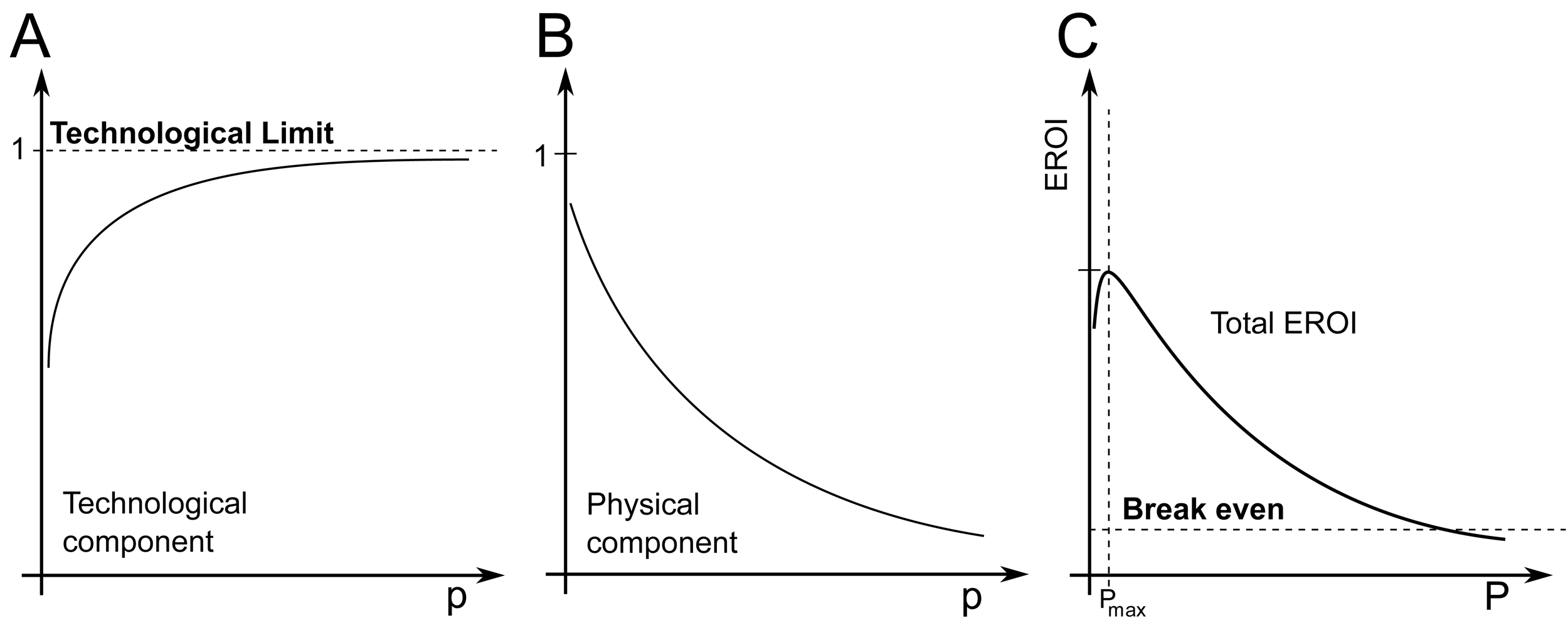
Within this work, we posit that this curve for the EROI is representative of not only Louisiana oil and gas but all non-renewable resources. We further assume that this EROI function is a product of two components: one technological, G, that serves to increase energy returns as a function of cumulative resource production, which serves as a proxy measure of experience, i.e., technological learning; and the other, H, diminishing energy returns due to declining physical resource quality. The function F(p) is depicted in Figure 6 along with the two components.
Where ε is a scaling factor that increases the EROI and p is cumulative production normalized to the size of the ultimately recoverable resource (URR). Within this work URR is assumed to be the total resource that may be recovered at positive net energy yield. In reality, ε and URR (or TP) would be used as parameters for scenario-based assessment or a Monte Carlo simulation. Normalised cumulative production, p is defined such that:
2.2. Technological Component
We assume that the technological component of the EROI function asymptotically increases as a function of production as shown in Figure 6. There are two factors that will influence this technological component of the EROI function: how much energy must be embodied within the equipment used to extract energy and how well that equipment performs the function of extracting energy from the environment. We assume that both of these factors are subject to strict physical limits. Firstly, that there is some minimum amount of energy that must be embodied in order to function as an energy extraction device, for instance the foundation of a wind turbine must successfully endure a large moment load. Secondly, there is a limit to how efficiently a device can extract energy. We further assume that, as a technology matures, i.e., as experience is gained, the processes involved become better equipped to use fewer resources: PV panels become more efficient and less energy intensive to produce; wind turbines become more efficient and increasing size allows exploitation of economies of scale. These factors serve to increase energy returns. However, it can be expected that these increases are subject to diminishing marginal returns as processes approach fundamental theoretical limits, such as the Lancaster-Betz limit in the case of wind turbines.
Technological learning curves (sometimes called cost or experience curves) track the costs of production as a function of production. These often follow an exponentially declining curve asymptotically approaching some lower limit. The progress ratio specifies the production taken for costs to halve. Between 1976 and 1992, the PV module price per watt of peak power, Wp, on the world market was 82% [19]. This means that the price halved for an increase in cumulative production of 82%. Lower financial production costs should correlate with lower values of embodied energy [4,20,21]. The specific form of the function is:
Here X represents the initial value of the immature technology and χ represents the rate of technological learning through experience, which will be dependent on a number of both social and physical factors. This rate is assumed constant.
2.3. Physical Depletion Component
The physical resource component of the EROI function is assumed to decrease to an asymptotic limit as a function of production, as shown in Figure 6. In general, those resources that offer the best returns (whether financial or energetic) are exploited first. Attention then turns to resources offering lower returns as production continues. In general the returns offered by an energy resource will depend upon the type of source, formation and depth of the reserve, hostility of the environment, distance from demand centers and any necessary safety or environmental measures. The costs of production often increase exponentially with increases in these factors [22]. The result is that the physical component of the EROI of the resource declines as a function of production. We assume that this decline in EROI, H will follow an exponential decay:
Here Φ represents the initial value of the physical component and φ represents the rate of degradation of the resource due to exploitation. Again this rate is assumed constant.
We justify this exponential curve by considering the distribution of energy resources. Some of these resources will offer large energy returns due to such factors as their energy density (e.g., grades of crude or coal), their ease of accessibility (e.g., depth of oil resources, on-shore vs. offshore), their proximity to demand centers (e.g., Texan vs. Polar oil) and possible other factors. The EROI of one particular source should be, if not normal, then most likely displays a positive skew, i.e., the median is less than the mean, as depicted in Figure 7. For example, there are more sites with lower average wind speeds than with higher wind speeds.
If we now assume that sites will be exploited as a function of their EROI, i.e., that those sites offering the best energy returns are exploited first, then we may now re-plot the cumulative distribution function as EROI depletion as a function of exploitation, i.e., production by rotating the axes and ranking the sites by EROI from highest to lowest.
2.4. Finding pmax
Since the EROI function for non-renewable resources is assumed to be a well-behaved function, the point pmax may be found via differentiation. pmax occurs at the value of p at which . Using the product rule finds that:
Differentiating G and H, gives:
Substituting Equations (6) and (7) into Equation (5) obtains:
Taking the natural logarithm of Equation (8) obtains:
2.5. The EROI Function for Renewable Resources
Unlike non-renewable sources, for which the EROI is solely a function of cumulative production, in the case of renewable energy sources the physical component of EROI is a function of annual production. The technological component will still be a function of cumulative production, which serves as a proxy measure for experience. In this case a reduction in production means that the EROI may “move back up the slope” of this physical component. In the interim, technology, which is a function of cumulative production, will have increased, further pushing up energy returns. This entails that the EROI of a renewable energy source is a path dependent function of production.
Decline in the physical component of EROI for renewable energy sources represents the likelihood of the most optimal sites being used earliest. For example, deployment of wind turbines presently occurs only in sites where the average wind speed is above some lower threshold and that are close to large demand centers to avoid the construction of large distribution networks. Over time, the availability of such optimal sites will decrease, pushing deployment into sites offering lower energy returns, which should be reflected in declining capacity factors over time.
3. Discussion
3.1. Supporting Evidence
We provide supporting evidence for the EROI function presented by considering wind and solar resources for the US as a case study. The technological component of the EROI may be increased by the production of wind turbines that are able to better extract energy from the passage of air. This increase is subject to an absolute physical limit represented by the Lancaster–Betz limit [23] which defines the maximum proportion of energy that may be extracted from a moving column of air as 16/27 ≃ 60%. Experience curves for wind farms show that long-term costs of energy production from wind have fallen exponentially as a function of cumulative energy production (a proxy for “experience”) [24].
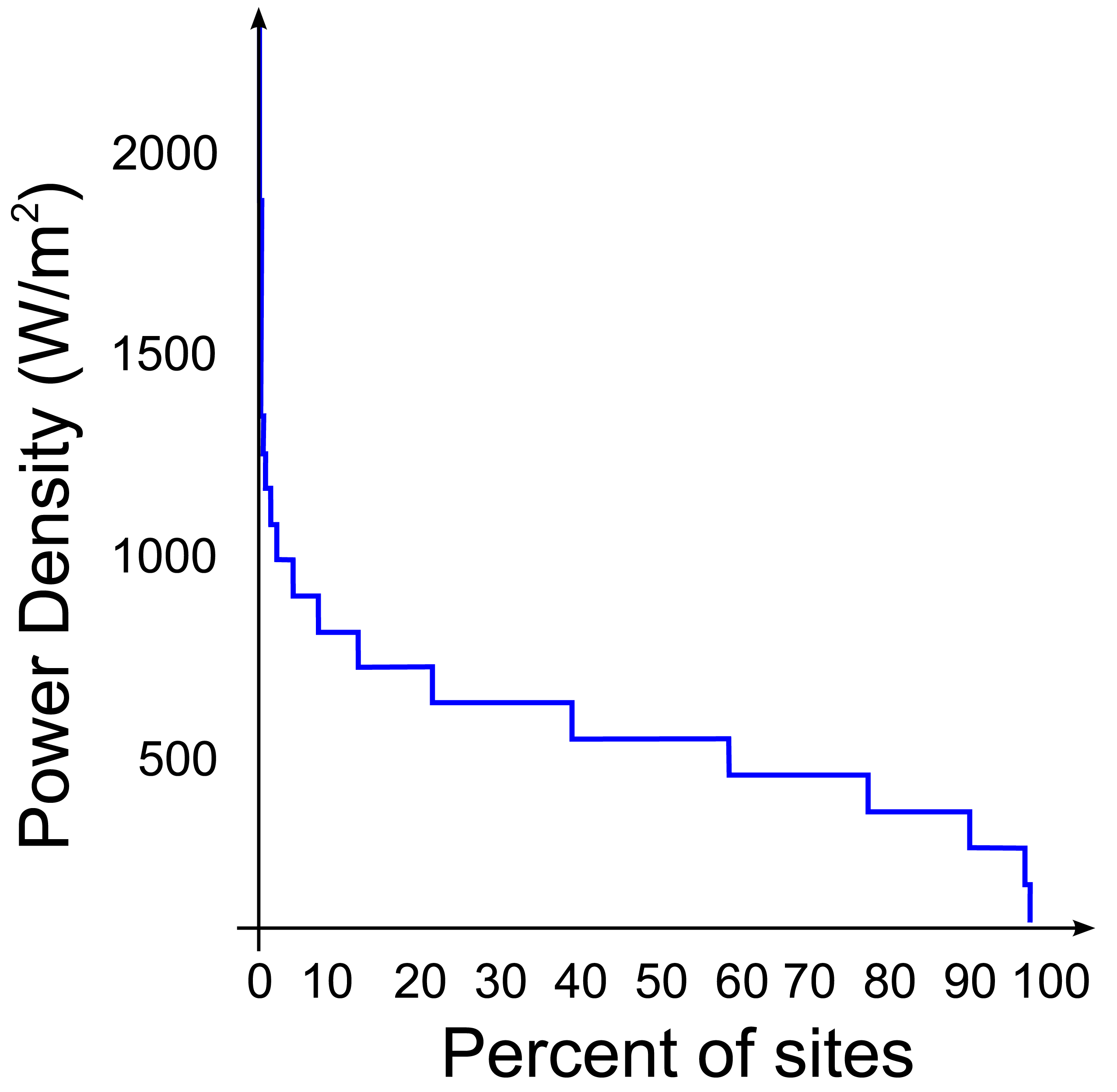
The resource base for wind has been extensively (and intensively) mapped in several regions of the world. The National Renewable Energy Laboratory (NREL) Western Wind Dataset [25] was used to produce a depletion curve of the US wind resource, ranked by power density (W/m2) shown in Figure 9. The power density of the wind resource initially declines exponentially as a function of land area, before dropping sharply below 500 W/m2.
NREL have also produced the National Solar Radiation Database (NSRDB), for the mainland US [26]. This data was used to produce a depletion curve of the US solar resource ranked by energy flux density (Wh/m2/day) shown in Figure 10. The energy flux density of the solar resource declines exponentially as a function of total land area from a maximum of just over 8,000 Wh/m2/day.
If we imagine the total resource being populated with identical turbines, each with a nominal constant embodied energy cost, κ [GJ/MW] and a nominal lifetime tL [yr] in such a way as to exploit the best sites first, the pattern of decline of the EROI as a function of total capacity installed [MW], will follow the pattern of the power density of the sites. An analogous case may be made of the solar resource.
Brandt (in press) [10] has made a long-term study of the EROI of oil production in California between 1955 and 2005. The EROI of this oil at the mine-mouth is shown in Figure 11. An exponentially decreasing curve is shown for comparison. The initial decline is greater than exponential.
3.2. What Use is the EROI Function?
Presently, long-term energy forecasting is done by predicting (or perhaps, more accurately, stipulating) long-term production costs for various energy supply and conversion technologies. This information is then used to optimize a “least-cost” energy system that meets the projected future energy demand. The problems associated with predicting something as volatile as production costs over timescales of decades is rarely discussed. The issue of declining net energy yields is never considered.
EROI defines the relationship between the amount of energy that must be embodied as human-made-capital (HMC) in order to produce energy and the amount of energy that HMC can produce. In Section 1.1.1., the EROI was defined as:
If the capital factor, κ, is now defined as:
Then, assuming that the annual production, ̇ is constant over the lifetime, L of the HMC, using Equations (10) and (11), the annual production can now be determined in terms of the HMC
Although energy dynamics are not well understood, since EROI is a physical property of an energy source, it should be easier to predict over long time periods than energy production costs (in monetary terms) or prices. The EROI function may then enable long-term energy forecasts to be made which are more accurate than those using solely price-based dynamics. Such a projection, based on the principles of energy analysis, will also automatically obey fundamental physical laws, such as the first and second laws of thermodynamics.
4. Conclusions
We have presented a top-down framework for determining the EROI of an energy source over the entire production cycle of an energy resource. This function allows production costs (in energetic terms) to be predicted into the future. This EROI function, coupled with a purely physical allocation function to allocate energy demand between different energy sources, will allow a new form of energy supply forecasting to be undertaken, based solely on physical principles.


Acknowledgments
This work would not have been possible without the support of the Department of Mechanical Engineering at the University of Canterbury and the Keith Laugesen Trust.
References
- Clerk-Maxwell, J. The Times; London; 31; August; 1950. [Google Scholar]
- Boustead, I.; Hancock, G.F. Handbook of Industrial Energy Analysis; Ellis Horwood: New York, NY, USA, 1979. [Google Scholar]
- Peet, J. Energy and the Ecological Economics of Sustainability; Island Press: Washington, DC, USA, 1992. [Google Scholar]
- Hall, C.A.; Cleveland, C.J.; Kaufman, R. Energy and Resource Quality: The Ecology of the Economic Process; John Wiley & Sons: Hoboken, NJ, USA, 1986. [Google Scholar]
- Cleveland, C.J. Net energy from the extraction of oil and gas in the United States. Energy 2005, 30, 769–782. [Google Scholar]
- Messner, S.; Strubegger, M. User's Guide for MESSAGE III; Technical report; IIASA: Laxenburg, Austria, 1995. [Google Scholar]
- Seebregts, A.J.; Goldstein, G.A.; Smekens, K. Energy/Environmental Modeling with the MARKAL Family of Models, Technical report. International Conference on Operations Research, Duisburg, Germany; 2001.
- OECD/IEA. World Energy Model—Methodology and Assumptions; Technical report; International Energy Agency: Paris, France, 2009. [Google Scholar]
- Baines, J.T.; Peet, J. The Dynamics of Energy Consumption: Changing Expectations for the Supply of Goods and Services; Department of Chemical Engineering: Christchurch, New Zealand, 1983. [Google Scholar]
- Brandt, A.R. The Effects of Oil Depletion on the Energy Efficiency of Oil Production: Bottom-up Estimates from the California Oil Industry. Sustainability 2011, 3, 1833–1854. [Google Scholar]
- Cleveland, C.J. An exploration of alternative measures of natural resource scarcity: The case of petroleum resources in the United States. Ecol. Econ. 1993, 7, 123–157. [Google Scholar]
- Hall, C.A.S.; Powers, R.; Schoenberg, W. Peak Oil, EROI, Investments and the economy in an uncertain future. In Biofuels, Solar and Wind as Renewable Energy Systems: Benefits and Risks; Pimentel, D., Ed.; Springer: Dordrecht, The Netherlands, 2008; pp. 109–132. [Google Scholar]
- Cleveland, C.J.; Costanza, R.; Hall, C.A.S.; Kaufmann, R. Energy and the US economy: A biophysical perspective. Science 1984, 225, 890–897. [Google Scholar]
- Leach, G. Energy and Food Production; IPC Science and Technology Press: Surrey, UK, 1976. [Google Scholar]
- Cleveland, C.J.; Kaufmann, R.K.; Stern, D.I. Aggregation and the role of energy in the economy. Ecol. Econ. 2000, 32, 301–317. [Google Scholar]
- Chapman, P.F.; Leach, G.; Slesser, M. Energy budgets. 2. Energy cost of fuels. Energy Policy 1974, 2, 231–243. [Google Scholar]
- Costanza, R.; Cleveland, C.J. Ultimate Recoverable Hydrocarbons in Louisiana: A Net Energy Approach; Louisiana State University: Baton Rouge, LA, USA, 1983. [Google Scholar]
- Hubbert, M.K. Nuclear Energy and the Fossil Fuels. In Drilling and Production Practice, Presented before the Spring Meeting of the Southern District Division of Production, American Petroleum Institute, Plaza Hotel, San Antonio, Texas, March 7–9, 1956; American Petroleum Institute, Shell Development Co.
- IEA. Experience Curves for Energy Technology Policy; Technical report; OECD/IEA: Paris, France, 2000. [Google Scholar]
- Costanza, R.; Cleveland, C.J. Value Theory and Energy. In Encyclopedia of Energy; Elsevier: New York, NY, USA, 2004; pp. 337–346. [Google Scholar]
- Liu, Z.; Koerwer, J.; Nemoto, J.; Imura, H. Physical energy cost serves as the “invisible hand” governing economic valuation: Direct evidence from biogeochemical data and the US metal market. Ecol. Econ. 2008, 67, 104–108. [Google Scholar]
- Cook, E. Limits to exploitation of nonrenewable resources. Science 1976, 191, 677–682. [Google Scholar]
- Rauh, A.; Seelert, W. The Betz optimum efficiency for windmills. Appl. Energy 1984, 17, 15–23. [Google Scholar]
- Junginger, M.; Faaij, A.; Turkenburg, W.C. Global experience curves for wind farms. Energy Policy 2005, 33, 133–150. [Google Scholar]
- NREL. Western Wind Dataset. http://www.nrel.gov/wind/integrationdatasets/western/data.html (accessed 10 February 2010).
- NREL. National Solar Radiation Database. http://rredc.nrel.gov/solar (accessed on 10 February 2010).
© 2011 by the authors; licensee MDPI, Basel, Switzerland. This article is an open access article distributed under the terms and conditions of the Creative Commons Attribution license(http://creativecommons.org/licenses/by/3.0/).
Share and Cite
Dale, M.; Krumdieck, S.; Bodger, P. A Dynamic Function for Energy Return on Investment. Sustainability 2011, 3, 1972-1985. https://doi.org/10.3390/su3101972
Dale M, Krumdieck S, Bodger P. A Dynamic Function for Energy Return on Investment. Sustainability. 2011; 3(10):1972-1985. https://doi.org/10.3390/su3101972
Chicago/Turabian StyleDale, Michael, Susan Krumdieck, and Pat Bodger. 2011. "A Dynamic Function for Energy Return on Investment" Sustainability 3, no. 10: 1972-1985. https://doi.org/10.3390/su3101972