Valuing Ecosystem Services with Fishery Rents: A Lumped-Parameter Approach to Hypoxia in the Neuse River Estuary

Abstract
: Valuing ecosystem services with microeconomic underpinnings presents challenges because these services typically constitute nonmarket values and contribute to human welfare indirectly through a series of ecological pathways that are dynamic, nonlinear, and difficult to quantify and link to appropriate economic spatial and temporal scales. This paper develops and demonstrates a method to value a portion of ecosystem services when a commercial fishery is dependent on the quality of estuarine habitat. Using a lumped-parameter, dynamic open access bioeconomic model that is spatially explicit and includes predator-prey interactions, this paper quantifies part of the value of improved ecosystem function in the Neuse River Estuary when nutrient pollution is reduced. Specifically, it traces the effects of nitrogen loading on the North Carolina commercial blue crab fishery by modeling the response of primary production and the subsequent impact on hypoxia (low dissolved oxygen). Hypoxia, in turn, affects blue crabs and their preferred prey. The discounted present value fishery rent increase from a 30% reduction in nitrogen loadings in the Neuse is $2.56 million, though this welfare estimate is fairly sensitive to some parameter values. Surprisingly, this number is not sensitive to initial conditions.1. Introduction
Valuing ecosystem services presents four challenges. First, many of the economic benefits generated are non-market. Second, ecosystem services typically contribute to human benefits indirectly. Humans may not value the service, per se, but something that it supports. For example, recreational anglers may value the fish in a stream but not necessarily the riparian habitat that support the fish population. Third, the links between ecosystem services and human values are dynamic and can be nonlinear, but economic valuation architecture is most developed for static problems. Finally, providing an empirical basis for ecosystem valuation involves multiple academic fields and profound spatial and temporal scale mismatches. To begin to address these challenges, one must simplify problems. In this paper, we highlight the strategic modeling choices that are involved in adapting a lumped-parameter bioeconomic model to study the valuation of ecosystem services.
Lumped-parameter approaches greatly simplify renewable resource dynamics by modeling a small number of states that depend on just a handful of parameters. While the overall goal of this research is to evaluate the strengths and weaknesses of lumped-parameter approaches to study the economic value of ecosystem services, we develop a particular model to highlight the research challenges that are involved in coupling economic and ecological models to answer a specific policy question. In our case, the specific policy issue is the tradeoff between nutrient loading in estuaries and the resulting effects on fisheries productivity. The simplifications in our lumped-parameter model balance conceptual knowledge about the estuarine ecology and the economics of the fishery with the data available for parameterizing each feature of the system.
We find that a lumped-parameter bioeconomic fisheries model is able to address each of the four challenges for valuing ecosystem services. First, we deal with a commercially valuable species. Hypoxia is not priced in the market, but fish that are affected by it do have market value. Our metric of economic value is fishery rent, which provides an exact welfare measure under some assumptions. Focusing on a producer problem in which we incorporate the opportunity cost of capital, we avoid many of the complications of nonmarket valuation such as substitution prospects, income effects, and identifying assumptions like weak complementarity. Implicitly, we assume that the market demand is perfectly elastic as is typical in bioeconomic models. Our work also responds to a recent National Research Council call for more research on the effects of nutrient pollution on commercially valuable coastal resources [1]. Second, the links between anthropogenic effects on ecosystem services and human values are modeled explicitly. The model traces the eutrophying effects of nutrient pollution to fishery outcomes starting with how nutrient loadings stimulate primary productivity in an estuary. Primary productivity affects dissolved oxygen levels and can lead to episodes of hypoxia (low oxygen) or anoxia (no oxygen). These episodes, in turn, cause migration of mobile crustaceans (like blue crabs, a harvested predator species) and mortality of sedentary benthic invertebrates (a non-harvested prey species). Fishing pressure responds to the overall abundance and spatial distribution of predators. Third, the paper models all states dynamically, and the paper begins to incorporate some key nonlinearities. Since rents are dissipated in the steady state under open access, the focus is entirely on transition dynamics. With an open access institutional structure, only a dynamic model has the ability to quantify welfare effects of policy changes that affect the environmental basis for the fishery. Finally, this paper attempts to integrate natural resource economics and multiple fields in ecology with common spatial and temporal scales.
The paper is organized as follows. Section 2 reviews the general policy context of estuarine nutrient pollution and discusses the specific background for the Neuse River Estuary and the blue crab fishery. Section 3 describes the lumped-parameter model and places it in the context of previous work in bioeconomics. Section 4 describes the model's parameterization. Section 5 presents results, and Section 6 discusses our results and outlines modeling issues for future research on coupled ecological and economic systems. The discussion section expands on the model description by explicitly considering some of the modeling tradeoffs in this application and for future work.
2. Policy Context
2.1. Nutrient Pollution, Hypoxia, and Fisheries
Nutrient pollution poses a number of threats to ecosystem services in coastal waters. Excess nutrients have been linked to increased primary productivity, hypoxia and anoxia, changes in the composition of the planktonic community, toxic algal blooms, decreased diversity in the trophic system, and increases in disease [1]. These problems are often interrelated. We focus on the link between primary productivity and low oxygen levels. As primary productivity increases in a water body, the system can become eutrophic, or over-enriched with organic material. Increased organic material stimulates oxygen demand. In an estuary, increased oxygen demand combined with stratification in the water column—a fresh water layer sitting on top of a salt water layer—can lead to hypoxia or anoxia in the bottom waters.
Hypoxia and anoxia can have substantial consequences for a wide range of species. In the Gulf of Mexico, which is experiencing large-scale hypoxic events, hypoxia affects the spatial distribution of species including Atlantic Croaker and brown shrimp [2], as well as sea turtles and marine mammals [3]. Hypoxia can lead to mortality of sedentary benthic organisms, many of which are prey species for demersal fish and shellfish [4]. Finally, hypoxic effects can reverberate through the entire food web. Baird et al. [5] suggest that hypoxia affects trophic efficiency by diverting energy from higher trophic levels to lower trophic levels.
In an estuarine environment, nitrogen is typically the limiting nutrient to growth in primary productivity, whereas phosphorous more often is limiting in lake environments [1]. Though there are exceptions, nitrogen limitation in estuaries is primarily attributable to the tendency for low nitrogen fixation by estuarine planktonic communities [1]. At low levels of nutrient loading, enhancing primary productivity may actually increase fishery productivity. However, once an estuary reaches eutrophic levels, additional primary productivity tends to decrease dissolved oxygen levels in the bottom waters of estuaries and lead to anoxic or hypoxic conditions. Caddy [6] depicts this stylized relationship between fishery productivity and different trophic states as an inverted-U shaped curve. At low (high) levels of nutrient enrichment, fishery productivity increases (decreases) with additional nutrient loading. Throughout this paper we assume that any policy-induced changes in nutrient loadings would not be enough to push the system out of a dystrophic or eutrophic state. That is, the system is always in the region in which fishery productivity is declining as more nutrients are added. Otherwise, reducing nutrient loadings could have perverse welfare impacts.
2.2. Nutrient Pollution in the Neuse River Watershed
Nutrient pollution in North Carolina's Neuse River Watershed has generated substantial public debate. Under the United States Clean Water Act, states are required to develop Total Maximum Daily Load (TMDL) plans for water bodies that do not meet water quality criteria, and these plans “must identify the amount by which point and nonpoint sources of pollution must be reduced in order for the water body to meet its stated water quality standards” [7]. The Neuse River Estuary is currently in a eutrophic state and, though there is some scientific debate on the subject, is thought to be nitrogen-limited. As a result, North Carolina has developed a TMDL to address nitrogen loadings [8]. We assume in the modeling that potential nitrogen reductions stemming from the TMDL are insufficient to flip the system from a eutrophic state to an oligotrophic state.
We examine commercial fishery productivity in the Neuse as one portion of the total economic benefits that would emerge from reduced nutrient pollution. Paerl et al. [9] document a connection between eutrophication in the Neuse Estuary and low dissolved oxygen levels. Several studies show how low oxygen levels, in turn, affect a range of demersal fish and shellfish species in the Neuse as well as their prey, including croaker, blue crab, spot, shrimp, menhaden, silver perch, southern flounder, weakfish, pinfish, hogchoker, and clams [10-13]. Powers et al. [12] highlight the potential cascade effects through the trophic system, while Eby and Crowder [10] and Eby et al. [13] emphasize how species avoidance of hypoxia can result in sublethal effects by altering their habitat use. In this paper, we particularly focus on how nutrient pollution affects the blue crab fishery in the Neuse River, Estuary, and in the contiguous Pamlico Sound. Our application is illustrative of a larger fisheries policy concern. In North Carolina, nine species that depend on estuarine soft-bottom habitat made up more than two thirds of total dockside commercial fisheries revenues statewide from 1994–1996 [4].
2.3. Hypoxia and the North Carolina Blue Crab Fishery
Blue crabs have both ecological and economic importance. Blue crabs can serve as a keystone predator in an estuary [14]. They have a complex life cycle with life stages spent in marine and estuarine environments [15]. Blue crabs eat a wide variety of foods including bivalves, crustaceans, fish, marine worms, plants, and detritus. They are preyed upon by a variety of species as well, including sea turtles, and they are prone to cannibalism of juveniles. When they are available, blue crabs prefer to eat bivalves such as clams [16]. Quantifying the ecological effects of hypoxia alone is complicated because multiple ecological pathways are involved. Adult blue crabs are highly mobile and can move up to 125 nautical miles in a season [14]. As a result, adult blue crabs can avoid hypoxia. In the Neuse Estuary, hypoxia varies over space and time. Blue crabs respond to hypoxic events by moving to shallow oxygenated areas near river edges [17]. When blue crabs migrate, they may experience increased competition for food sources. Preferred blue crab prey, in contrast, are sedentary and can experience mortality as a result of hypoxia. Thus, there is a direct effect of hypoxia that stimulates blue crab migration and an indirect effect that reduces prey availability in the hypoxic area.
The blue crab fishery is the most valuable commercial fishery in North Carolina and consists of three product types sold dockside: hard shell, soft shell, and peeler. Nominal ex vessel revenues across all three categories totaled $34.44 million in 2002 and peaked at $44.96 million in 1998. The bulk of landings are hard shell, accounting for 96.6% of the 37,592,317 pounds landed in 2002. Blue crab landings in 2003 accounted for more than one third of all landed value in North Carolina commercial fisheries. Figure 1 depicts catch and real revenues (in 2002 dollars) from 1950–2002. To compute real revenues, we used the Bureau of Labor Statistics CPI All Urban Consumers for 1950–1977 and switch to CPI South Size D (the smallest rural category) when it becomes available in 1978. The landings time series data are from the NOAA Fisheries Commercial Landings Data Website [18]. Burgess and Bianchi [19] report recent figures on fishermen, vessels, and trips. The number of fishermen landing hard blue crab ranged from 2,161 in 1994 to a peak of 2,338 in 1997 and down to 1,550 in 2002. Vessels follow a similar pattern: 2,474 in 1994, a peak of 3,418 in 1996, and down to 1,900 in 2002. Trips also followed this pattern (109,603 in 1994, a peak of 119,557 in 1998, and 82,633 in 2002). The North Carolina blue crab fishery is conducted mostly during the summer season with 88% of harvest taking place in May through October [20].
The North Carolina blue crab fishery is a large share of the total for the Eastern United States. North Carolina blue crab comprised 13.46% of total blue crab landings from 1950–1993 and 24.24% of landings from 1994–2002 [20]. In spite of the high value of the blue crab fishery for North Carolina and the value of blue crabs elsewhere, we are unaware of any prior bioeconomic analysis to examine blue crab fishery regulation. Upadhyaya, Larson, and Mixon [21] use a simultaneous equations econometric model to explore “costs” of regulation in the Maryland blue crab fishery, but they in no way account for the bioeconomic nature of the problem.
Current and proposed management tools for the North Carolina blue crab fishery are all open access alternatives [20]. We rely on the draft blue crab fishery management plan [20] for all of the information in this paragraph. Current management includes a license requirement, a minimum size limit, blue crab spawning sanctuaries, and several gear restrictions including limitations on crab dredging and specifications on crab pots. Some gear restrictions are spatially and temporally varying as well. The North Carolina General Assembly (NCGA) placed a moratorium on new licenses that took effect 1 July 1994. The moratorium and the existing crab licenses were scheduled to expire 30 June 1999. NCGA established an interim crab license until October 2000 while discussion of effort management continued. Meanwhile, the Fishery Reform Act of 1997 capped the Standard Commercial Fishing License starting 1 July 1999, but the cap was not able to limit entry on blue crab. In September of 1999, the Marine Fisheries Commission decided that it would not continue to pursue limited entry and would focus only on open access options. Thus, limited entry for blue crab effectively expired when the interim blue crab license expired in 2000.
3. Model Description
The lumped-parameter model is a system of ordinary differential equations that represents changes in the stock of nutrients, algae levels, spatially explicit populations of the blue crab and prey availability, total fishing effort, and the spatial distribution of fishing effort. The goal of this system is to trace changes in nutrient loadings all the way through to impacts on fishery rents, which provide a meaningful economic metric. However, changes in nutrient levels do not directly affect fishery harvest. Instead, nutrient loadings coupled with hydrodynamics alter the ecosystem that supports the fishery. Specifically, increased nutrients stimulate the production of algae in the estuary and provide a precursor to hypoxia. Hypoxic events, which tend to be spatially delineated in the estuary, affect prey availability and can induce blue crab emigration from hypoxic to oxygenated zones. Fishing pressure, in turn, responds to the overall status of the blue crab resource and its spatial distribution. Thus, changes in the fishery that are attributable to nutrient loadings can only be uncovered as they filter through complex ecological and economic dynamics. In this sense, the model aims to measure market benefits of ecosystem services that have not been measured before. Nevertheless, we acknowledge that analysts may also be interested in simpler metrics like additional catch or revenue that a fishery can sustain in the long run with a reduction in nutrient pollution. Our model measures these changes as well.
Nutrient loadings and algal growth have simple model structures. Denoting t as time, the stock of nutrients (N(t)) in the estuary evolve according to:
For purposes of optimizing the model (in future analysis), it will be necessary to preserve the time-dependency of loadings. Optimizing the model, which is beyond the scope of this paper, would involve setting up and solving an optimal control problem with at least three controls, six states, and a variety of non-negativity constraints. However, to gain some qualitative insights initially, we assume that nutrient loadings are constant over time, L(t) = L̅, and any policy change would modify this constant rate. Obviously, this simplification ignores seasonality in loading. However, given that nutrient accumulation does not translate instantaneously into algal blooms, considering an annual average is appropriate. The robustness of the assumption can thus be evaluated by the extent of inter-annual variation in loadings. We model algae (A(t)) with logistic growth where the intrinsic growth rate is normalized to one, and the carrying capacity is a linear scaling of nutrient stock with a parameter μ:
In this way, the long-run stock of algal blooms is limited by the nutrient stock, and the dynamics of algal growth are influenced by the dynamics of nutrient accumulation. Note that with constant nutrient loadings, the steady-state nutrient stock and algae stock are: N∞ = L̅/ϖ and A∞ = μL̅/ϖ.
A potentially interesting extension of this model would be to incorporate algal biomass hysteresis. The residence time of organic matter in estuaries involves fresh and saltwater interchange as well as the physics of sediment transport [25], so even if algae carrying capacity is reduced in response to nutrient loadings, it could take some time to cycle the oxygen demand in sediments out of the system. To account for this possibility, we might modify (2) to follow the nutrient recycling in (1'):
For tractability, we model a two-patch bioeconomic system to study the effects of hypoxia on the blue crab fishery. In this lumped-parameter model, a patch can be viewed as either shallow versus deep water or estuary versus the sound. Both interpretations are consistent with the effects that we get, and the difference would be in the parameterization. We treat Patch 1 as the estuary and Patch 2 as the Pamlico Sound. Due to depth, currents, and other aspects of hydrodynamics, we assume that Patch 1 is susceptible to algal blooms and thus can experience hypoxia. As such, the algae stock in (2) is assigned to Patch 1. In contrast, we assume that Patch 2 does not have excess algae growth and hence has no hypoxia. Another way of interpreting the model is that Patch 2 has only background effects of algae, and when a hypoxic event occurs, Patch 2 is relatively more oxygenated than Patch 1. Because we limit algae growth to Patch 1, this model is inappropriate for considering doomsday scenarios in which nutrient loadings are so severe that the entire estuary is hypoxic or anoxic at all times. One can imagine that such a scenario would destroy the environmental basis for the fishery (at least the basis in the Neuse) and comparisons among policy alternatives with marginal changes in loadings would be less meaningful than global ones (in the mathematical sense). In the population dynamics below, we also assume that the patches are of equal size. This assumption could be relaxed by introducing additional parameters.
There are four state equations that describe the population dynamics: predators in each patch and prey in each patch. Blue crabs are the predators and are subject to fishing mortality and environmental limits on their abundance that include prey abundance. Prey in the model are a composite of infaunal species, mostly clams, that are unable to move across patches. Hence, we explicitly model preferred prey of adult blue crabs. We do not model potentially differential impacts of hypoxia on the various components of their diets, preferred or otherwise, and assume that hypoxia affects preferred prey but does not affect non-preferred prey. Since blue crabs are scavengers and eat a wide variety of organic material at various life stages [26], we implicitly model non-preferred prey using a lumped-parameter approach. Denote predators and prey in Patch i as Xi(t) and Yi(t) respectively. There are five components of predator population dynamics. The first three components follow Ragozin and Brown [27] and Wilen and Brown [28] and model logistic growth of each species separate from the Lotka-Volterra predator-prey interaction terms. These authors neither consider spatial differentiation of the resource nor explicit environmental effects on the resource. In our setting, this is equivalent to assuming no hypoxia and no spatial connectivity between patches. The crab populations would thus evolve according to:
The two last components of predator population dynamics account for the direct effects of hypoxia and spatial connectivity of the patches. Both of these terms affect predator migration between the patches. Our approach is in the spirit of previous bioeconomic models of habitat dependence [29-33], but in our model environmental quality degradation does not reduce the availability of the harvested species directly; stocks are affected indirectly through migration and prey availability. We do not explicitly model hydrodynamic conditions that cause hypoxic events. Instead, we model average responses to hypoxia precursors, namely algae. This approach is useful in that it preserves the deterministic structure of the model and avoids the complications of seasonality and additional state equations to describe water column dynamics. It does come at a cost, since our model has the potential to miss important aspects of hypoxia that are associated with extreme events (in the tails of the distribution), and averaging over the episodic nature of hypoxia creates a disconnect between empirical observations of the physical environment and model parameters. With these caveats in mind, we posit the percent change in predator population in Patch 1 is a decreasing function of algae and for simplicity specify a linear relationship with a single parameter ξ Modeling the direct effect of hypoxia as emigration from deoxygenated areas, as opposed to retarded growth or increased natural mortality, follows the empirical findings of Selberg, Eby, and Crowder [17] and Eby and Crowder [10]. Beyond hypoxic-induced immigration, we model migration as a linear function of the difference in relative prey density across the two patches. If prey per unit of predator is larger in Patch 1 (Patch 2) than in Patch 2 (Patch 1), predators migrate towards Patch 1 (Patch 2). This patch framework draws on Sanchirico and Wilen [34] but arguably is less lumped in that there is a structural determinant of predator flows, namely the prey densities. With these two components added to (3), and denoting responsiveness to relative prey density as ϕ, the population dynamics for predators in each patch are:
This form ensures that absolute prey differentials do not lead to migration of more than the population in a patch, and migration is limited when both predator and prey populations are scaled up or down.
The population dynamics of the preferred prey species have some similarity in structure to predator population dynamics, but the effects of hypoxia are quite different. Like in equations (4) and (5), prey in each patch has a logistic growth component and a predator-prey interaction component. As a lumped-parameter model, we ignore the possibility that the composition of different prey species changes over time. Without loss of generality, we normalize prey carrying capacity to one such that steady-state prey populations are one in each patch when there is no hypoxia and no predation. Because prey are not harvested, we are not interested in the level but rather the population as a share of its potential. Unlike the predator state equations, there is no harvest of the preferred prey. Also unlike predator dynamics, the prey are stationary, i.e., they do not migrate from one patch to the other. For blue crab, this assumption is reasonable because most blue crab prey are bivalves that burrow into the sand and are unable to migrate purposefully. Larval dispersal of prey between patches is a potential confounding factor, but lumped-parameter models of this sort are not capable of modeling life history characteristics explicitly. Finally, since the prey are stationary, we model the effects of hypoxia as creating extra prey mortality in Patch 1. An additional source of prey mortality that we do not model is the possibility that hypoxic conditions can increase prey susceptibility to predators by decreasing their burial depths [35]. The model could be extended to include this effect by endogenizing the predation parameters α and β, but this extension would add nonlinearity and nonconvexity. This extension, coupled with economic dynamics, could create the perverse situation in which increasing nutrient loadings would be welfare improving for the fishery. Mathematically, this appears the same as the prey having two predators, one of which is algae. Patch 1 prey dynamics have all three components, while Patch 2 prey state dynamics have just two because we assume that hypoxia has only background effects on Patch 2:
Note that we have just three additional parameters to describe the prey state equations: intrinsic growth of prey (ry), predator-prey interaction coefficient (β), and hypoxia-related prey deaths (ρ). All of these are lumped-parameters, but ρ is unique to the model in this paper and requires additional attention. The model does not explicitly track sediment oxygen demand. Instead, it assumes that sediment oxygen demand is implicit in the stock of algae. Thus, ρ captures two important features of the system: (1) the effect of primary productivity on sediment oxygen demand and (2) the effect of sediment oxygen demand on prey mortality. The first of these effects is implicitly folded into the parameter ξ in (4) and (5) as well, but as will be discussed in the next section, there is no information available to pin down ξ, so a wide range of values must be considered. In contrast, we will be able to provide some empirical basis for the two components of ρ. By construction, our model assumes a form of natural insurance in that patch 2 is sheltered from the direct effects of hypoxia.
Turning to the economics, there are two key states that we track and that together with an assumption on the production technology will close the model and determine bioeconomic outcomes. These states are the spatially-explicit levels of fishing effort (E1(t) and E2(t)), and in the case of blue crab, can be thought of as the number of traps in each patch at each point in time. Following Smith [36] and Smith and Wilen [37], it is useful to reformulate these states as total fishing effort E(t) and its spatial distribution. With just two patches, knowing total effort and the share of effort in one patch (πi) fully determines the total amount of effort allocated to each patch. Formally,
The blue crab fishery in North Carolina has been essentially open access for most of its history. There are some limits on gear technology but no formal limits on entry, and though there was a temporary moratorium on new permits, we assume that it was not in effect long enough to fundamentally alter the open access dynamics of the fishery. Thus, total effort in the model follows a dynamic open access rent dissipation model originally formulated by V. Smith [38,39] and empirically estimated for the fur seal fishery in Wilen [40]. Total fishery rents (Πtotal(t)) are simply the difference between fishing revenues and fishing costs where c represents a combined constant marginal cost of fishing equipment and opportunity cost of time, and δ captures the opportunity cost of investing in the equipment (cost of capital and depreciation):
Note that we also assume a constant price (p) and that crab fishermen are price-takers. Price-taking is not a very strong assumption given that blue crab are harvested in many regions along the east coast of the U.S., the North Carolina harvest in recent years is about a quarter of the total, the Neuse and Pamlico combined harvest is roughly one third of the NC harvest, and changes in nutrient pollution are not likely to affect harvest magnitudes greatly. We can revisit this issue if the model produces large chanes in quantities harvested that would question the price-taking assumption. Whether aggregate harvest in this fishery could influence regional prices enough to warrant endogenizing price is an empirical question beyond the scope of this research. Constant price is an analytical convenience for assessing the theoretical properties of the model, but in future work the simulation could incorporate a price path that tracks actual price data with an additional state equation. For evaluating present value rents later in the paper, we will denote r as the discount rate and recognize that the opportunity cost of investment is related to the discount rate such that δ'(r) > 0. Thus, the link between the cost of capital and the more general concept of time value of money is the reason to separate c and δ as separate components of the cost of effort. Following open access theory [38-41], total effort evolves according to average rent per unit of effort rather than marginal rent:
Note that in the steady-state, as in Sanchirico and Wilen [34], this effort adjustment condition is simply a two-patch generalization of the familiar condition that catch-per-unit-effort equals the cost-price ratio.
The share of effort in each patch responds to relative density of blue crabs according to a logistic probability density function. For Patch 1, effort share is:
This approach is consistent with the empirical literature on broad fishery choice [42] as well as specific fishing location choice [36]. Selberg, Eby, and Crowder [17] conduct a survey of blue crabbers in the Neuse and find that they recognize low oxygen water and move their crab pots in response to environmental conditions. Since blue crabs essentially crowd into the oxygenated areas during a hypoxic event, there may be an effect on the catchability coefficient q, and not just an increase in CPUE associated with an increase in patch 2 biomass (holding effort constant). We use just a single parameter θ to model the responsiveness (over space) to different levels of abundance. Because the logit model is only identified up to scale, implicitly this parameter captures something about the amount of information contained in expected catches relative to the overall variance that influences fishing behavior. If there were no information (i.e., the error dominates completely), we would expect harvesters on average to distribute themselves uniformly over space. We do not incorporate any sluggish adjustment over time for simplicity, but this extension could be done as Smith [43] does empirically to model state dependence. So that we can stack our system of differential equations, we take the time derivative of (13) and simplify to obtain:
To close the model, we assume a simple Schaefer (1957) production function for harvest:
Using (10), we can simplify (16) to:
To summarize, we now have a description of the system that is a function of seven state variables [N(t), A(t), X1(t), X2(t), Y1(t), Y2(t),E(t), and π1(t)], parameters, and initial conditions.
4. Parameterizing the Model
Parameterizing the model described above presents numerous challenges. For some of the parameters, empirical estimates simply do not exist or the data are of such poor quality that meaningful statistical inference is not feasible. For others, empirical estimates in the ecology literature do exist but apply to vastly different spatial and temporal scales. In many cases, the studies that provide empirical estimates involve very different model structures and not just different scales. Finally, some parameters pose units problems as well. With all of these caveats in mind, by parameterizing the model we seek to accomplish five objectives: (1) demonstrate our methodology for quantifying partial ecosystem service values; (2) provide an initial estimate of the magnitude of value (albeit one with considerable uncertainty); (3) explore qualitative insights from the model and whether parameter values affect qualitative patterns in the dynamics; (4) identify parameters to which the value of ecosystem services is sensitive; and (5) illustrate challenges in coupling ecological and economic models for policy analysis. Our actual figures for present value rents should be interpreted with caution. Appendix A provides a brief overview of the parameterization in table form. Our strategy is to draw directly from the empirical literature to the extent possible. When estimates are unavailable, we back out parameters that are internally consistent with empirical estimates for other quantities in the model.
For parameter values in (1) and (2) and hypoxia-related parameters in (4)–(6), we rely on work from Mark Borsuk's Ph.D. Dissertation at Duke University and related work with co-authors. Borsuk develops a Bayesian hierarchical network model that addresses a number of ecological and hydrological features of the nutrient pollution in the Neuse River and Estuary [44,45], called Neu-BERN. This model is one of three models featured in the Neuse TMDL to evaluate the consequences of reducing nitrogen loadings in the Neuse [8]. One advantage of Neu-BERN is that it describes a range of outcomes probabilistically rather than just providing a point estimate. Another advantage is that Neu-BERN is able model various features of the system without forcing a common temporal or spatial scale. Features enter as nodes, which are modeled as marginal probabilities, and outcomes that involve multiple nodes are joint probabilities. One disadvantage, however, is that it is not equipped to handle dynamics across nodes. In our context, dynamics are essential because the fishery is rent dissipating; steady-state rents with and without nitrogen reduction are identically equal to zero by construction. The welfare effects of water quality improvements can only be recovered from the transition to the steady state. Thus, the model structure of Neu-BERN is inappropriate for our purposes, but it provides useful empirical information. In building a dynamic model with common spatial and temporal scales, we sacrifice the scale flexibility of Neu-BERN and the ability to make probabilistic statements about outcomes. We can still evaluate different combinations of parameters through sensitivity analysis but cannot say which outcomes are more likely in a statistical sense.
In (1), we rely on static models to choose two parameters: baseline loading (L̅) and nitrogen decay rate ω. While seemingly straightforward, baseline loading is complicated by variability in the flow of the Neuse River. Stow and Borsuk [46] compute flow-adjusted nitrogen concentration various locations in the Neuse in the 1980s and 1990s. The median nitrogen concentrations across locations are approximately 1.3 mg/L in 1991–1994 prior to any policy-induced reductions in nitrogen. Neither these authors nor the Neuse TMDL [8] accounts for lags in the decay of nitrogen stock. This suggests that nitrogen decay rate ω might be relatively rapid. We choose ω = 0.95 based on our judgment and adjust L̅ = 1.2 so that the steady-state nitrogen concentration is approximately 1.3.
The parameter μ in (2) maps steady-state nitrogen concentration into algal carrying capacity. Borsuk, Stow, and Reckhow [47] estimate five log-linear regression models of chlorophyll response to temperature, total nitrogen, and several transformations of water flow. Each model represents a different part of the Neuse. Given the functional form, the parameter on total nitrogen is a percentage change in chlorophyll in response to a one unit change in nitrogen. This fits directly into our model with the caveat that our model implicitly builds in a lag in chlorophyll response. The implicit intrinsic growth rate of chlorophyll in our model is 1.0, so approach the steady state is quite fast. The point estimates of the five models range from 0.22 to 0.70 with standard errors as small as 0.15 and as large as 0.62. We choose 0.40 as an initial point estimate.
We assume that algal accumulation affects dissolved oxygen concentrations instantaneously, again with the caveat that our model does not explore the episodic nature of hypoxia. Since the effect is instantaneous, it is not necessary to model algae accumulation and dissolved oxygen depletion separately. The parameters ξ and ρ are lumped in that sense; they combine the marginal effects of primary productivity (measured as algae levels) on dissolved oxygen levels and the effect of dissolved oxygen levels on the outcome of interest (migration for the blue crab and mortality for their clam prey). As modeled, empirical estimates do not appear in the ecology literature, but we can use the decomposed effects to construct plausible parameter values. The first of these decomposed effects is the link between algae and dissolved oxygen.
Linking primary productivity to dissolved oxygen levels with some empirical basis inevitably confronts spatial and temporal scale mismatches as well as units problems. The spatial scale of the ecological data is often much finer than the model in this paper, so some aggregation is necessary. Also, these data are typically not collected with dynamics in mind. When dynamics do enter, they may be fast dynamics that do not match the economic dynamics. For example, Borsuk, Stow, Leuttich, Paerl, and Pinckney [48] look at oxygen dynamics in the Neuse within-season and focus on vertical stratification of the water column. Our model is simply not equipped to incorporate the episodic nature of vertical stratification and the corresponding time scale of days. To deal with all of these issues, we compute an elasticity based on the model in Borsuk, Stow, Higdon, and Reckhow [49] and evaluate it at the mean levels of parameters and concentrations of organic matter and sediment oxygen demand across the Neuse River Estuary. The calculation implicitly assumes an instantaneous conversion of organic matter (attributable to primary production) into sediment oxygen demand.
Equation 9 in Borsuk, Stow, Higdon, and Reckhow [49] provides a simplified expression for Sediment Oxygen Demand (SOD) as a function of carbon loadings (L), depth (h), and parameters a, b, and k:
Since our primary productivity is scaled to have a maximum of approximately one, depending on the nutrient concentration, an elasticity will eliminate the units problem (at least as a first order approximation). The elasticity of SOD with respect to K (ε) is:
Note that a cancels out entirely in the elasticity. Median parameters values in the Neuse Estuary are: b = 0.785 and k = 0.00085. Taking the average over Lower, Middle, and Upper Neuse, we have depth as hbar = 3.0 and Lbar = 43.2. Thus, evaluated at the means, ε = 0.7071.
We next consider a range of sediment oxygen demand levels from 100% of the baseline down to 50% of the baseline and we compute (in percentage terms) the corresponding decreases in primary productivity from the baseline (100%) using 1/ε. Finally, we linearize this relationship to get a marginal oxygen demand of 0.57 with a standard error of 0.03. Since oxygen demand in the system is an instantaneous response, we can simply multiply 0.57 times the blue crab responsiveness to dissolved oxygen to construct ξ. Similarly, we can build up prey mortality (ρ) by multiplying mortality as a function of dissolved oxygen by 0.79.
Selberg, Eby, and Crowder [17] and Eby and Crowder [10] have identified some oxygen threshold concentrations for blue crabs, but we are not yet able to connect this information to the parameter ξ. For now, we examine the sensitivity to results over a broad range of parameter values and maintain parameter values that ensure that migration biomass from patch 1 cannot exceed the quantity of biomass in patch 1. We begin with a moderate level of ξ = 0.5.
To link dissolved oxygen to prey mortality in (6), we adapt empirical results from Borsuk, Powers, and Peterson [50]. These authors estimate a survival model of clams in the Neuse in response to changing dissolved oxygen levels. We subtract mean survival probabilities from their Table 3 to obtain mean cumulative mortality at three different levels of dissolved oxygen (0% reduction, 25% reduction, and 50% reduction). Then we regress baseline oxygen demand (1, 0.75, 0.5) on mortality (0.89, 0.77, 0.53) to obtain a slope of 0.72 and an intercept of .19. Although results are not statistically significant with just three observations, the mortality relationship is well-approximated by a linear function (R2 = 0.97) in this range of dissolved oxygen. When we include mean and median results from Borsuk, Powers, and Peterson [50] Table 3, we have six observations in the regression and slope and intercept parameters are statistically significant at the 5% level. The slope parameter adjusts upward to 0.74, the intercept still rounds to 0.19, and the R2 drops to 0.95. To summarize, 0.72 will be the mortality component of p, and we will use the intercept to guide selection of intrinsic growth of prey. Combining the two marginal effects in p, we have ρ = 0.79 × 0.72 = 0.57.
We rely on a stock assessment of North Carolina blue crab to estimate the logistic growth parameters in (4) and (5). Eggleston, Johnson, and Hightower [51], EJH hereafter, consider intrinsic growth rates for blue crab that range from 0.20 to 2.0 and estimate carrying capacities that range from 102.29 million pounds to 526.60 million pounds in a surplus production model based on crab catch and pot data from 1953–2002. Note that smaller growth rates correspond to larger carrying capacities. We first adjust downward the range of blue crab intrinsic growth to account for the positive effect of predation in (4) and (5). Our low, medium, and high values are 0.05, 0.75, and 1.5.
Next we need to interpolate a relevant carrying capacity for the part of the NC fishery that we are studying. EJH estimate that 7% of the fishery is conducted in the Neuse River and 28% in the Pamlico Sound, which is the water body that the Neuse Estuary opens into. We assume that our model applies to this total 35% of the fishery. Thus, we assume that the range of steady-state crab population combined across the two patches is 35% of the carrying capacity range in EJH. In the absence of hypoxia, and assuming that our two patches are of equal size, half of this capacity is then allocated to each patch. This steady-state population reflects predation, but with no hypoxia, the two patches are equal and all of the migration terms in (4) and (5) drop out.
We next turn to finding values for kx and α. Because of the Lotka-Volterra dynamics, the steady-state cycles and there is no analytical solution to Ẋ(t) = Ẏ(t) = 0 . Thus, we can fix one predator-prey parameter, hold one state near the steady state (near Ẏ(t) = 0) and back out parameters using Ẋ(t)=0 . The parameter that we fix is β=0.001. This allows for blue crab predation to account for between 3.6% and 19.5% of clam mortality. We take this range and add it to the maximum mortality from dissolved oxygen depletion (0.72) and the mortality intercept (0.19) to obtain a range of intrinsic growth rates for clam prey (1.11, 0.97, 0.95) that would prevent total stock collapse under the worst-case in-sample hypoxia scenario. Again, our purpose here is to explore marginal effects not the possibility for catastrophic changes if the Neuse River becomes far more eutrophic. Using Excel's nonlinear solver, we impose Ẋ(t) = 0 to recover parameters that correspond to low, medium and high values for rx. For kx we have 78.07, 25.85, and 14.50; for α we have 0.025, 0.375, and 0.743. We acknowledge that this procedure is very ad hoc, but the need to apply such a procedure illustrates the mismatch of existing empirical estimates and a model structure needed to answer the policy question at hand.
We have no existing literature to guide our choice of the final biological parameter, ϕ. The idea of this parameter is to link patches on the basis of relative prey availability. An interpretation of this lumped-parameter mechanism is that it captures an incentive for blue crab to re-colonize hypoxic areas after the hypoxic event ends. It is naturally bounded by 0 on the low end, and we assume that it is bounded on the high end by relative scaling of prey and predator carrying capacities in the model. We thus consider values of 5, 50, and 150.
We now turn to the economic parameters of the model. For parameterizing the model, we convert all past prices and costs to 2002 dollars using the BLS CPI South Size D (the smallest rural classification) for 1978–2002. Prior to 1978, this CPI was not available, so we use CPI All Urban Consumers. In the simulations, we use a five-year weighted average price (1998–2002) across the three product categories (hard shell, soft shell, and peeler), so p = 0.87. The parameters c, δ, and γ do not appear in the literature, and there is insufficient data to estimate them econometrically with any degree of confidence. We rely on a detailed study of the Chesapeake Bay blue crab fishery [52] for total cost on a per trip basis. Their average total costs range from $229 to $279 in 1999 dollars for full-time watermen. Rhodes, Lipton, and Shabman [52] use a survey to obtain these cost estimates and compute them in two different ways: adding up the various components of costs and explicitly asking watermen the minimum revenues needed to justify a fishing trip. They caution that whether these costs include opportunity cost of time depends on how the respondents interpreted the question. We convert to 2002 dollars and proceed with these estimates as the sum of c and δ. Until we conduct policy experiments modifying the discount rate, the decomposition of c and δ does not matter, so we report initial estimates in the next section without breaking down these parameters.
By regressing lagged CPUE and lagged NC unemployment (to account for variability in opportunity cost), we can estimate the share of average total cost that is exclusive of opportunity cost of time to be 70%. We do not use the implied values for costs from the regression because nothing is statistically significant, and we have only 7 years of trip data. We run the regression simply as an initial attempt to decompose cost components. If we assume a discount rate r = 0.05, a constant rate of depreciation of 0.1, and take the average fixed cost numbers from Rhodes, Lipton, and Shabman [52], we can estimate all of the relevant cost components. For the low ATC (240.45), Average Fixed Cost = 52.50, opportunity cost of time is 74.84, and user cost (δ) is 7.875, which implies c = 232.575. For the high ATC (292.95), Average Fixed Cost = 85.05, opportunity cost of time is 91.18, and user cost (δ) is 12.758, which implies c = 280.192. Again we need to stress that for the results reported in the next section, this decomposition does not matter; it will only matter when we consider policy experiments in which the discount rate is allowed to change. At first blush, our numbers for opportunity cost of time seem reasonable. They imply that alternative employment, on average, would be worth roughly $10 per hour. Median household income for NC blue crabbers is in the $50,001–$75,000 bracket [20]. Assuming the crabber earns half of this income, this implies an hourly average wage ranging from (based on 2000-hour work year) $12.50 to $18.75. These numbers are well above the implied opportunity cost of time.
To parameterize the speed of adjustment γ, we need to make additional assumptions. First, because trip data are not available for a long enough period (and are influenced by the license moratorium), we need to backcast trips based on crab pot data. To do this backcasting, we assume total pots per trip is a stable relationship over 1984–present. We then take the overlap period of pot and trip data (1994–2002), exclude 1995–1997 because of possible over-reporting of pots, and take the average pots per trip (crab pot data was provided by Sean McKenna of NCDENR, Division of Marine Fisheries). Second, we take the implied trips from 1984–2002 and compute one-period-ahead forecasts based on the rent dissipating effort equation (12). Finally, we solve for γ by minimizing the sum of squared deviations. For the two sets of c and δ, the implied γ is surprisingly similar (45.37 and 46.81).
We follow a similar one-period-ahead forecast procedure to parameterize catchability q. Here we set initial stock at carrying capacity, backcast trips all the way to 1953 using the procedure above, and search for a q that qualitatively matches the pattern of catch, and quantitatively matches the total over the time horizon as well as individual periods. This routine is similar to the calibration of catchability in Smith and Wilen [37], in which no single objective over the time horizon adequately captures the nature of the calibration problem. For medium parameter values, we have q = 0.000003.
The final economic parameter is the spatial adjustment parameter θ. Selberg, Eby, and Crowder [17] show that blue crabbers are responsive in moving their crab pots to varying conditions but do not have a quantitative measure of how responsive they are. Thus, we rely on estimates from Smith and Wilen [53], who report a short-run spatial adjustment elasticity of that ranges from 0.35 to 3.1 for spatial responsiveness in the sea urchin dive fishery with 11 patches, implying a range of θ between 0.39 and 3.41. With just two patches, the elasticity of spatial adjustment in patch i is θ (1 – πi), so ceteris paribus it is inevitably smaller. If we assume uniform spatial distribution of effort, the re-scaling of the implied θ is 0.55, so the range is 0.21 to 1.88. We choose 0.4 as the medium level because the larger elasticities in Smith and Wilen [53] correspond to infrequently visited patches.
We assume that the system starts at the steady-state values for the biophysical states N(t) and A(t) because the dynamics are fast relative to the economic dynamics, and there are no feedbacks from the fishery, i.e., the steady states are recursive. Thus, choosing these initial conditions for N(t) and A(t) is straightforward. With the parameters above, we have N(0) = 1.2632 and A(0) = 0.50526.
We choose initial population levels for predators and prey in each patch to correspond to half of the logistic growth carrying capacity parameters. For predators, we thus choose X1(0) = X2(0) = 0.5 × kx = 12.92 million pounds (for medium parameter values). Prey populations in each patch are scaled to the (0,1) interval in the absence of predation and hypoxia. We thus choose Y1(0) = Y2(0) = 0.5.
For initial economic parameters, we choose total effort to be 35% of the total trips in the NC blue crab fishery averaged over 2000–2002. This yields E(0) = 32,077. For the share in each patch, we treat the patches as representing equal size. Thus, to explore the behavior of the model, we start the patch share at π(0) = π2(0) = 0.5.
Because our parameterization draws on a wide range of studies and adapts parameters from different model types, we do not have a clear roadmap for incorporating parameter uncertainty. That is, we cannot characterize the joint distribution of our parameters and draw repeatedly from that joint distribution to simulate the model. This is a limitation in comparison to the Neu-BERN model. However, what we gain from this sacrifice is the ability to incorporate dynamics explicitly on a scale that matters for human impacts.
5. Results
We simulate the system in continuous time using Matlab's Ordinary Differential Equation Solver (ODE45). We consider a 30% reduction in nitrogen loadings, which is what the Neuse TMDL calls for [8]. While our possible range of parameter values spans the range in EJH, for brevity we present a full set of results based on the medium levels of parameters. At these levels, with initial conditions set to half of the kx and implicit ky parameters, and assuming a real discount rate of 2.5%, a 30% reduction in nitrogen loadings sustained over a 50-year time period generates an increases in present value rents of $2.56 million, a total catch increase of 12.4 million pounds, and a total increase in trips of 91,000. In percentage terms, these are increases of 7.7%, 3.6%, and 2.9% for rents, catch, and effort respectively. It is worth noting here that our welfare estimates assume that there are no consumer surplus gains from the policy changes. This implicitly assumes that the blue crab market demand is perfectly elastic in the range of policy-induced supply shifts. One could approximate consumer surplus changes by econometrically estimating the slope of the crab market demand, but this is beyond the scope of our paper.
Since fishery rent may not be the only metric that matters to policy-makers, we can examine the long-run impacts on catch and effort from the policy change. We take average catch and effort over the last two years of our 50-year simulation as an approximation of long-run effects. The baseline long-run catch and effort per year are 5.7 million pounds and 60,662 trips respectively. The increases from the 30% nitrogen reduction are 230,000 pounds and 2,270 trips. Trips per year is in the neighborhood of 60, which averages across full-time and part-time fishermen. This suggests that the water quality improvement would support 38 additional fishermen in the Neuse and Pamlico Sound in the long run.
Table 1 analyzes the sensitivity of our results (aggregated over 50 years) to the parameter μ, which maps nitrogen stock into the carrying capacity of algae. The results in bold repeat those described in the previous paragraph. The 30% reduction policy increases rents at an increasing rate as the parameter μ increases. Fortunately, we do have some empirical basis for μ, but there is still considerable uncertainty. Table 2 analyzes sensitivity to changes in the per trip cost (c + δ). Again, the results in bold repeat those described in the previous paragraph. In sharp contrast to Table 1, the welfare impacts of the 30% reduction policy are virtually unaffected by differences in per trip cost. The change in total effort is stable across this range of costs as well. The main difference across the cost range is the total catch in the system. With lower costs, short-run rents are higher but are dissipated faster; there is more effort entry early in the time horizon. This excess entry tends to reduce the blue crab stocks, and the system can sustain a lower catch in the medium and long runs. Because of discounting, the losses in the medium run–recall that long-run rents always tend to zero–under the lower cost scenario are offset by the short-run rent gains. Also of interest is that stocks are driven to zero if the per trip cost is low enough. We found that this can occur with a per trip cost below $100.
Table 3 explores the sensitivity of results to the economic speed of adjustment of total fishing effort, γ. As in Tables 2 and 3, our point estimate results are in bold. In percentage terms, the speed of adjustment has virtually no impact on the results of the policy change for rents, catch, and effort. In magnitudes, slower speed of adjustment corresponds to larger baseline rents and thus larger gains from the reduction in nutrient pollution. When fishing effort responds faster, rents are dissipated faster. Given that the initial conditions start the system off with positive rents, faster rent dissipation means smaller present value rents. Faster effort response also means that stocks are driven down more quickly and can sustain a high catch for a shorter period of time. As a result, total catch is declining in γ. Finally, the magnitude of total effort changes very little in response to γ. In the short run, effort is higher, but in the long run, effort is lower as a result of depleted stocks. Thus, the short- and long-run effects on effort are nearly offset.
Figures 2–4 depict the system dynamics under the no reduction scenario. The qualitative patterns in figures for the 30% reduction scenario are similar, but the levels change in ways that conform to expectations. Figure 2 shows the paths of patch 1 and patch 2 blue crab populations and the populations of their preferred prey. They start from the same levels, the blue crab patch 1 population is approaching a lower level than the patch 2 population. The long cycles reflect a combination of predator-prey dynamics, the economic dynamics in the system, and initial conditions. The dampening amplitudes are a result of large overshooting in the economic sector and are consistent with other empirical open access results (e.g., [40]). In contrast, prey populations approach steady-state levels smoothly. However, examining the data underlying these graphs reveal predator-prey cycles. The amplitudes of these cycles, however, are swamped by the importance of initial conditions. Figure 3 shows how fishing effort responds dynamically. The top panel depicts the long entry-exit cycles that are characteristic of open access fisheries with fixed costs. Effort share in patch 1 is cycling around 0.37, which ultimately reflects the impacts of nutrient pollution. Even at the level of spatial distribution of fishing effort, it takes quite some time for the system to settle down. Looking at this panel more closely, we see the presence of both long and short dynamics. The long dynamics have a period that matches that of the overall entry-exit pattern. The short dynamics reflect responsiveness to small fluctuations in blue crab populations as a result of predation, migration due to relative prey availability, and migration due to hypoxia. The bottom panel of Figure 3 tracks total catch over time and present value rents over time. Catch cycles with a similar magnitude to fishing effort. Amplitude differences reflect the concurrence of effort and biomass changes. There appear to be short dynamics as well, but they are less pronounced than they are in effort share. Present value rents have a similar pattern, but the effect of discounting dampens cycles rather dramatically after the first fifteen years.
Figure 4 shows blue crab migration decomposed into its two separate components. The first panel tracks migration due to relative prey abundance. The large-amplitude cycles reflect low point in the blue crab populations. When a predator population is in a trough, relative prey availability can change substantially over a short period. Interestingly, the large cycles die out in year 20, but medium-sized cycles begin again around year 35. Blue crab migration due to hypoxia, as shown in the bottom panel, is smoother throughout. The pattern reflects long dynamic swings in the patch 1 blue crab population. Phase portraits (not shown here) of predator and prey populations show the usual cycling pattern of Lotka-Volterra models.
Figures 5 and 6 look at the dynamic paths of rent differences and effort differences under the 30% reduction policy. In Figure 5, the most pronounced effect is the short-run rent difference. Although cycles continue well into the future, most of the rent impacts of the policy have materialized by the 15th year. This is partly a reflection of discounting but also a reflection of the open access rent dissipating process. Interestingly, rent differences are negative initially. This likely is a reflection of over- and undershooting somewhere in the system. If we break Figure 5 into three sections, we essentially have a period of short-run transitory rents, a period of bioeconomic overshooting, and a period of rent dissipation near the bioeconomic steady state. The period of short-run transitory rents gives us an indication of how much value the environmental quality change can generate. In an optimized system, this initial positive cycle would be dampened and stretched out over an infinite horizon. Interpreting Figure 6 is less straightforward. The long cycle in this figure appears to be stretched. This may reflect the long cycles in the two scenarios being out of phase combined with short dynamics as well. Even once present value rents have nearly approached zero, there is still a fair amount of movement in the effort difference.
Naturally, one must ask how much of the changes in rents, catch, and effort are an artifact of initial conditions. To explore this issue, we use the same parameter values to run the model out 300 years with no reduction in nitrogen. We save the last year state values (approximate steady states) as initial conditions. Then we look at 50-year scenarios with and without the 30% reduction. With these initial conditions, a 30% reduction in nitrogen loadings sustained over a 50-year time period generates an increases in present value rents of $2.75 million, a total catch increase of 13.4 million pounds, and a total increase in trips of 100,000. These numbers are similar to the simulation beginning at half of carrying capacities. The effect of nitrogen loadings in magnitude does not appear to be sensitive to initial conditions. Across the two sets of initial conditions, we obtain essentially the same estimate for welfare improvements from a 30% nitrogen reduction.
6. Discussion
This paper develops a method to estimate the value of ecosystem services that support a commercial fishery with a solid microeconomic foundation. In particular, it uses a lumped-parameter dynamic bioeconomic model to evaluate welfare changes from reduced nutrient pollution, which enhances ecosystem function by increasing dissolved oxygen, in terms of fishery rents. We illustrate the model using the North Carolina commercial blue crab fishery and examining the proposed 30% nitrogen reduction in the Neuse River Watershed. In this discussion, we provide additional context as well as some caveats for interpreting our ecosystem service values, and we suggest future research directions linking economic and ecological models by examining our own strategic modeling decisions. Along the way, we highlight the ways in which we lump parameters and how these ways are likely to affect policy analysis.
6.1. Interpreting the Value of Ecosystem Services
Our best point estimate for the value of a 30% reduction in nitrogen loadings is $2.56 million, though this figure ranges from $195,000 to $7.51 million simply by varying parameters within what we consider to be a reasonable range. The TMDL plan does not require a benefit-cost analysis, so we have little information on the magnitude of total economic benefits. Still, it is worth asking why this number is so small. To understand our value of a 30% nitrogen reduction, it is essential to highlight the coexistence of other value changes from that same reduction, the importance of fisheries management institutions in driving the value, and the large degree of parameter uncertainty in our model.
The ecosystem service values that we measure are only a subset of the total that might emerge from a 30% reduction in nitrogen. Our values are partial largely because not all of the ecosystem values contribute to blue crabs, and not all values are rivals in consumption. That is, capturing value in the blue crab fishery associated with reduced nutrient pollution does not necessarily diminish values of other ecosystem services associated with the same water quality improvement. Reducing hypoxia by decreasing nitrogen loading in the Neuse may benefit other commercial fisheries as well as the blue crab fishery. Nitrogen reductions may also contribute to ecosystem values through trophic interactions that are not captured by benefits to fisheries. However, these values have not yet been quantified and arguably are more difficult to pin down.
Previous economic research has analyzed how nitrogen reductions could enhance the value of recreational fisheries and other forms of recreation in the Neuse. In fact, the hypothesis that reduced nitrogen loadings will generate recreational fishery benefits is consistent with static non-market valuation studies of the Neuse [54-56]. Interestingly, a 30% nitrogen reduction appears to pass a benefit-cost test based solely on recreational values [57]. Thus, prior estimates of total recreational benefits dwarf the benefits to the most valuable commercial fishery in the state. The extent to which recreational and commercial benefits are rivals with each other is an empirical question and one that is important for many fisheries around the world. We expect that the extent of rivalry will depend largely on institutional arrangements that limit access to the resource.
Perhaps the most important reason that our welfare estimate seems small is the institutional structure of the blue crab fishery. North Carolina blue crabs are managed under open access, and open access dissipates rents in the long run. As a result, any values that an environmental quality improvement generates are necessarily transitory; no sustainable value can persist under open access. In contrast, under optimal management the economic benefits of reduced nitrogen would not be dissipated. The present value welfare change could thus be considerably larger. However, without analyzing optimal fisheries management, it is difficult to speculate on how big these benefits would be. Naturally, the next step in this research agenda would be to derive the optimal policy and compute present value rents under different nitrogen reduction scenarios.
Our application illustrates the importance of institutions as a broad theme in the valuation of environmental resources. The value and not just the behavioral effect of an environmental change is actually contingent on the institutional context. McConnell and Strand [30] make this point in a conceptual model of water quality dependence of a commercial fishery, while Freeman [58] makes this point in a static model of the Gulf Coast blue crab fishery that provides empirical welfare estimates of productivity changes in response to wetland acreage changes. The economic value of a water quality improvement in our case cannot be isolated from the open access setting any more than it can be isolated from the ecological processes. Krutilla and Eckstein [59] first called attention to the importance of physical and economic interdependence in project evaluation. In a recent tribute article, Smith [60] summarizes John Krutilla's thinking about these economic, physical, and institutional interdependencies, writing that they “are not separable influences to what can be expected with policy intervention. They interact with each other altering the incentives and responses of people inside and outside markets” (p. 1174).
The interaction of institutions and value of ecosystem services naturally raises the question of how recreational blue crab fishing would be affected by different combinations of water quality changes and institutional settings. Under open access, recreators may contribute to the dissipation of gains from improved water quality by putting additional pressure on crab stocks. Similarly, potential gains from rationalizing the commercial crab fishery—and capturing more value from the crab resource itself and from the water quality improvement—could be offset to some degree by maintaining open access in the recreational sector. Optimal management would jointly consider recreational harvest, commercial harvest, and water quality. The conceptual bioeconomic literature on recreational and commercial fisheries emphasizes the jointness of recreational and commercial sectors in determining optimal management [61-63].
Just as the open access assumption is a critical determinant of the dollar figure that we find for rent changes, the assumption of a representative agent is important as well. In that sense, the economic parameters in our model are lumped; they represent averages over the population of fishermen. Since economic parameters enter nonlinearly into present value rent sums, even introducing heterogeneity through parameters with symmetric distributions could affect outcomes. Moreover, Johnson and Libecap [64] argue that with heterogeneous agents, rents are zero in open access “only for the marginal fisherman.” (p. 1012). Here again we see the importance of the institutional and larger economic context of a policy change. Whether or not there is fishing skill heterogeneity, fishermen almost certainly have varying opportunity costs that depend on connections to local economies, and these opportunity cost differences can affect the aggregate exertion of fishing effort. Though beyond the scope of this paper, introducing heterogeneity in the harvest sector could generate an additional source of rents attributable to differences in fishing skill.
Beyond the institutional considerations described above, it is worth interpreting our ecosystem values as a first order approximation purely for quantitative reasons. Since no prior study has been able to quantify the economic benefits to the blue crab fishery from reduced nutrient loading, or to any fishery for that matter, there does not exist a benchmark against which we can compare the magnitude of our result. Given that and the way that we parameterize the model, our quantitative results should be interpreted with caution, especially for non-marginal changes. First, we have only begun to explore the parameter space. Conducting a thorough sensitivity analysis will likely involve thousands of simulations. Second, all of the parameters in our empirical application involve substantial uncertainty. Most are adapted from studies that do not have a model like ours in mind; they deal with substantially different temporal and spatial scales, they involve different units, and the some of them have different functional forms. The model is quite sensitive to the parameter that maps nitrogen stock into steady-state algae. This parameter enters nonlinearly, so this sensitivity is not surprising. In terms of scientific interpretation, we need sound, statistically-based description of how much nitrogen affects chlorophyll production that, in turn, reduces dissolved oxygen levels. Most of the scientific literature that deals with this question addresses ecological dynamics that are too short (e.g., intra-seasonal) for the type of long-run welfare analysis that we are conducting here.
Units of measurement could affect the results. For two parameters, we use elasticities to overcome units problems, but these elasticities must be evaluated at particular levels of the variables. We assume mean levels, so any non-marginal change that pushes the system far from these values could also affect the elasticities. One might reasonably argue that a 30% reduction in nitrogen loadings is not a marginal change, but it is important to consider that the effects of nitrogen on blue crab filter through many ecological pathways, and nutrients are not the sole environmental basis for the fishery. To the extent that some of the ecological pathways dampen the effect of nitrogen rather than amplify it, we believe that our model works reasonably well. Overall, fruitful directions for future research thus include reducing uncertainty about key parameters and improving the match between ecological studies and economic studies in terms of spatial scale, temporal scale, and functional form.
6.2. Linking Economics and Ecology
Many strategic modeling assumptions are necessary to trace a water quality improvement all the way to changes in fishery rents. It is useful for discussion to divide them roughly into assumptions that determine three types of effects: the direction of effects, the magnitude of effects, and the timing of effects. In dynamic models in which some metric is measured in present value, magnitude and timing are interrelated. For instance, pushing back a nominal gain several periods (a timing change) ultimately reduces the present value magnitude. To the extent that we can separate these two types of effects, we focus on nominal changes to categorize them. For lumped parameters, timing and magnitude are typically inseparable.
6.2.1. Direction of Effects
The assumptions that determine the direction (or sign) of policy impacts are functional forms and parameter signs. Most of these assumptions are implicit parameter signs that are not controversial. Some examples include positive intrinsic growth, positive carrying capacity, positive prices, positive costs of fishing effort, and a negative predator-prey interaction in the prey state equations. We characterize most of our ecological system by linear processes. To the extent that nonlinearity is introduced, we have used predominantly convex modeling and have focused on monotonic relationships between nutrients and fishery outcomes. Dasgupta and Maler [22] caution against relying too heavily on convex models. Thus, important extensions would include introducing non-convexities and relaxing some of the linear assumptions in the model. This issue goes beyond matching functional form in our model to functional form in empirical ecological papers; it raises the possibility of multiple equilibria, chaos, and perverse welfare consequences of policy changes.
Predator-prey responses to hypoxia are an important determinant of the direction of policy impacts. Though we do not model it, a potentially important nonmonotonicity may exist for these responses. Taylor and Eggleston [35] find that there are sublethal effects in blue crab preferred prey at low levels of hypoxia. Specifically, clams burrow less deeply when there is low oxygen and thus can experience increased predation. In the short run, this effect could stimulate growth of blue crabs, and considering the effect of discounting, could generate a perverse welfare impact from reducing hypoxia. In other words, worsening hypoxia could temporarily stimulate blue crab stocks and lead to short-run fishery gains. In the long run, sustainable harvest would be lower, but given the rent dissipating nature of open access, long-run rents would still be zero.
A related issue is our exclusive focus on the negative relationship between fishery productivity and nutrient enrichment. Formally, this restriction comes through our linear scaling of nutrient stock into algal carrying capacity. However, as Caddy [6] showed, the negative relationship between nutrient enrichment and fishery productivity is just one part of a globally non-monotonic relationship. Our model is not equipped to analyze the impacts of increased nutrients in an under-enriched environment. There is a parallel here to the concept of hormesis in the dose-response literature on environmental pollution control. Hormetic substances are harmful at high doses but beneficial at low doses, and existence of hormesis can raise or lower optimal pollution control depending on control costs [65]. Adapting the literature on hormesis to a dynamic bioeconomic setting is an interesting direction for future research that presents analytical and empirical challenges.
The impact of hypoxia on fishing behavior could also affect the direction of policy impacts. As modeled, hypoxia can only reduce welfare. However, it is possible that blue crab avoidance of hypoxia could increase catchability in the non-hypoxic patch. The idea here is that since blue crabs essentially crowd into the oxygenated areas during a hypoxic event, there may an increase in catch-per-unit-effort beyond that associated with an increase in patch 2 biomass (holding effort constant). This effect would potentially create perverse outcomes: short-term rent increases probably at the expense of long-term catch. In an open access setting, whether the increase in catchability would be welfare-improving would then hinge on the discount rate, and there is at least a theoretical possibility that decreasing hypoxia by reducing nutrient pollution would be welfare-reducing. Here again the importance of institutions is critical. Under a rationalized fishery, the positive catchability effect would be offset some (possibly all) by a negative stock effect that reduces long-run profitability. With open access, long-run profitability is zero either way. Overall, the possibility of perverse welfare effects presents interesting challenges for future research on valuing ecosystem services by linking economic and ecological models.
6.2.2. Magnitude of Effects
A key determinant of the magnitude of changes from a water quality improvement is the way in which we model space. As described in Section IV, our model generates a type of natural insurance. Because patch 2 is not prone to hypoxia, there is a limit to how much nutrient pollution can affect our system. In the limiting case with severe nutrient pollution in patch 1, all blue crabs migrate to patch 2, and the entire fishery is conducted in patch 2. Even under open access, patch 2 serves as a contingent resource that insures against a complete collapse due to pollution. In an analogous common property exploitation problem, availability of groundwater can be viewed as a contingent resource when surface deliveries are stochastic [66]. Our assumption matches a spatial interpretation in which patch 1 is the estuary and patch 2 is the contiguous Pamlico Sound. Nutrient levels affect oxygen in the estuary, but there is enough mixing in the Sound to eliminate the nutrient-induced oxygen depletion, at least in the range of current loadings.
One could generalize our model to allow for differential hypoxic effects across patches by introducing an additional parameter. This would allow for an alternative spatial interpretation that corresponds to deep versus shallow water within the estuary. Of course, all of the biological parameterization would change to reflect the fact that the estuary alone is a smaller portion of the statewide crab fishery. Given our empirical setting, we argue that our parsimonious two-patch model provides meaningful estimates for policy analysis. For developing modeling strategies more generally, the researcher must ask: does interest lie in different spatial segments of the same water body or in connected water bodies that pollution may affect differentially. If the latter, is it possible to treat one as the index water body with no (or only background) effects of pollution?
Among the most striking results from our model is the lack of sensitivity to initial conditions; that is, initial conditions only have a tiny impact on the magnitude of policy outcomes. Upon closer examination, it is a combination of assumptions that drives this result, namely the linearity of the nitrogen stock and steady-state algae, the linearity of direct hypoxic effects, and the nature of open access rent-dissipating models. For the linearity assumptions, whether stocks are big or small and whether total effort is big or small, the nitrogen reduction leads to the same increase and approximate timing in fishery productivity. The magnitude and timing do not depend on the state of the system. This is the same intuition for why the open access structure matters. For a given increase in available rents associated with a productivity increase from less pollution, there is an extra amount of effort required to dissipate these rents. The level required does not depend on the level of existing effort because the Schaefer production function restricts the exponent on effort to one. Thus, the existing level of effort does not affect the difference between revenues and costs when the stock responds to the policy change; the difference is proportional to the increase in the stock whether existing effort is high or low.
Our assumption of constant real price affects the magnitudes of several metrics that interest policy-makers. Given that blue crabs in the Neuse constitute a small share of overall east coast blue crab harvest, making price endogenous is unlikely to be worth the effort. However, we can easily introduce some exogenous growth in real prices to examine sensitivity to the constant price assumption. With 2% growth in real price, baseline rents (with no water quality improvement) are higher compared to constant prices, and the policy change generates a somewhat higher rent increase of $2.92 million. Total effort and long-run effort are also higher, but total catch and long-run catch are lower. This reflects the cost-price ratio effect in open access models.
6.2.3. Timing of Effects
One of the key assumptions in our model is how quickly nutrient pollution can be cycled out of the system when loadings are reduced. We assume that nitrogen decays rapidly, and as a result, gains from reduced loadings materialize quickly. In reality, this decay could be slow. The consequence for policy impacts is that benefits to the fishery from nutrient reduction materialize later. We simulate a nitrogen decay rate of 0.475 (compared to our baseline of 0.95) and find that the present value rent increase from the policy change is $146,900 less than in the baseline. One of the features of the model that limits the size of this timing effect is the bioeconomic overshooting. When the system overshoots, rents go negative for a period. Pushing the positive rents back several periods also pushes back the negative rent overshooting period, so there is a loss from positive rent delays that is partially offset by the gain from negative rent delays. There may also be hysteresis in oxygen demand. This could be modeled with hysteresis in nutrients, as in Brock and Starrett [23] and Maler, Xepapadeas, and de Zeeuw [67] for shallow lakes, or hysteresis in the algae population. For an estuarine environment, it may be more realistic to do the latter. Without modeling hysteresis formally, the implications are less clear than simply speeding up or slowing down nutrient decay. However, we can speculate that measured from the status quo hysteresis would both delay the policy impact of a nitrogen reduction and decrease its magnitude. Both of these effects would reduce the present value benefits of the policy. On the other hand, hysteresis would amplify the negative consequences of increased loadings, causing a greater benefit from avoiding additional loadings.
A related timing effect is our assumption about the intrinsic growth of algae. Since we do not specify a species of algae, our model corresponds to some generic representative algae (or representative primary productivity). By assuming an intrinsic growth rate of 1.0, we assume that algae responds rapidly to changes in nutrient levels. A smaller intrinsic growth parameter would slow responsiveness, delay benefits, and thus lower the present value benefits of the policy change. On the other hand, a smaller parameter would also delay damages from increased nutrient levels and reduce the present value benefits of avoiding more pollution. With cycling due to open access, the net effect could have either sign. A simulation in which the intrinsic growth of algae is assumed to be 0.5 demonstrates this intuition; present value rent increase from the policy change is roughly $95,000 larger than in simulations using intrinsic growth of 1.0.
Both of these timing effects illustrate a key difference between the traditional static approach to valuing water quality improvements and the dynamic bioeconomic approach in our paper. The static approach typically assumes a direct effect of water quality on behavior. When data on fish stocks are available, researchers can decompose this direct effect into the effect of water quality on the fish stock and the effect of fish stocks on behavior. The relationship between water quality and fish stocks is still a reduced-form one. Static models by construction assume that the effects of a water quality improvement are instantaneous, and only a handful of researchers are able to relax the instantaneous effect assumption because doing so requires panel data. In contrast, our approach does not separate the timing of ecological impacts from the structure of the ecology and the resulting behavioral changes. These interdependencies can interact in nonlinear ways, and treating them as a sequence of reduced-form relationships could lead to different policy inferences.
6.2.4. Lumped Parameters—Timing, Magnitude, and the Partial Reduced Form of a Coupled System
Economic speed of adjustment dramatically affects the timing and magnitude of gains from a policy change. When the harvest sector adjusts rapidly (slowly), baseline rents are small (large), and rent gains from the policy change are also small (large). Upon closer examination, this speed of adjustment parameter is also a lumped parameter. It reflects fixed costs of entry, constraints on available labor in the short run, as well constraints on available non-fishing employment in the short run. It is useful to lump these effects together in a dynamic fisheries model because they usually cannot be measured individually, whereas the speed of adjustment can be estimated econometrically as in Wilen [40].
Our model implicitly assumes homogenous harvesters following the bioeconomic literature on which it builds. Extending our model to account for heterogeneity would be an interesting direction for future research. Real fisheries involve fleets with heterogenous vessels, captain skill, and opportunity costs of time. In such a setting, there could be important distributional consequences of a water quality improvement. One can debate about whether rents that accrue to captain skill or other fixed inputs should be considered resource rents. So, research in this area would need to disaggregate rents in a manner that clearly separates infra-marginal rents from resource rents in the homogenous model.
As in any simulation model, the choice of a deterministic or a stochastic model can be a key strategic decision. Here we use a deterministic model for two reasons. First, since our problem is a new one in the literature, we seek to generate baseline insights with deterministic modeling. Second, point estimates are often more useful for policy-makers. One can debate the relative merits of stochastic and deterministic modeling in general or for any particular setting, but doing this is beyond the scope of our paper. Instead, we point to one aspect of the bio-physical system that raises questions about deterministic modeling for this problem. Incidence of hypoxia does not unfold on a continuous basis but rather as a series of events governed by changes in hydrodynamic conditions. As an alternative to our approach, one could model the data generating process of these events. Since the effects of hypoxia enter linearly into our model, the importance of modeling stochasticity would likely hinge on the asymmetry of distributions characterizing hypoxic events and thickness of the tails. Adapting a lumped-parameter model to deal with the episodic nature of hypoxia would be an interesting direction for future research.
The ways in which our ecological parameters lump effects could matter even if results do not appear sensitive to the particular parameters. The hypoxia-related prey mortality parameter is a good example. This parameter captures the effect of increased algae on dissolved oxygen and the effect of dissolved oxygen on prey mortality in a multiplicative fashion. If both components of this parameter are understated or overstated, the combined change could be substantial. This is a general problem of lumped-parameter models.
Our treatment of space illustrates parameter lumping in a different way. There is no parameter that explicitly governs patch size. Rather, patch size is implicitly governed by population parameters. When predator carrying capacities are equal to each other across both patches and prey carrying capacities are as well, patch sizes are implicitly of equal size. But this illustrates a broader point about logistic-growth models: that these models implicitly characterize the quantity of available habitat. Logistic growth models also implicitly capture natural mortality through the interaction of carrying capacity and intrinsic growth.
Of particular interest in a model of nutrient pollution is what the prey death parameter means when population parameters are lumped. Hypoxia can in principle lead to death and growth retardation. Over time at the population level, a lumped-parameter model cannot distinguish these effects, but it may not need to. The policy implications from a more detailed model that includes the effects of oxygen depletion on respiration of individual organisms may provide the same qualitative results and similar quantitative ones. Researchers need to ask how much would modeling the biological mechanism affect results, and is it worth the additional effort?
The most important strategic modeling assumption is the actual choice of a lumped-parameter model. A rough analogy can be drawn to an econometric choice among a structural model, a reduced form model, and a partial reduced-form. In other words, there exists a compromise choice between the two extremes. There may be ways of using structural information to provide over-identifying restrictions on a reduced-form model, and these in turn provide efficiency gains without having to estimate the structural model [68]. If we draw the analogy from statistical efficiency to the provision of scientific information, then a lumped-parameter model is like this partial reduced form. The true structure provides guidance for what we might consider in a lumped-parameter model. Clearly, the field of population dynamics has moved beyond the logistic growth model towards models with many parameters that are more closely tied to observable quantities in nature. Yet, logistic growth can impose some restrictions that are consistent with the state of knowledge in many biological systems, and as in our model, features can be added to the basic structure to accommodate new knowledge. Our assumption of prey separability for the blue crabs is an example of this approach. We know that blue crabs have widely varying diets, but we also know that their preferred prey are particularly susceptible to hypoxia. Rather than discarding this information, we use it. We do not capture all of the ecosystem effects of hypoxia, but instead we capture ones that we think are of first-order importance for the blue crab fishery. Unfortunately, at the population level, we know very little quantitatively about interaction of blue crabs with their preferred prey. This raises the question: with problems quantifying population-level parameters, do researchers need to work from the ground up, presumably with some bioenergetic approach?
The benefits of a lumped-parameter model are straightforward, but the costs are still in question. On the benefits side, the model provides a parsimonious representation of a coupled system that is consistent with the general structure of the problem. This parsimony allows a researcher to adapt the model in transparent ways to answer policy questions directly. For modeling coupled ecological and economic systems, which parameters are lumped and how they are lumped clearly makes a difference. The strategic modeling question is the following: is it worth the costs—in terms of intellectual effort and potentially lost precision—to aggregate over different model types and data scales to arrive at values for a lumped-parameter representation? If we begin with an ecological model and attach an economic one, we may answer this question differently than if we begin with an economic model and attach an ecological one. The optimal choice along the continuum of models comprised of more or less lumped parameters will balance the benefits of additional accuracy and precision with the additional costs of developing a more detailed model in terms of time, resources, and identification challenges. Striking the proper balance between these benefits and costs may be the greatest current challenge for bringing together ecological and economic models for the purpose of valuing ecosystem services.


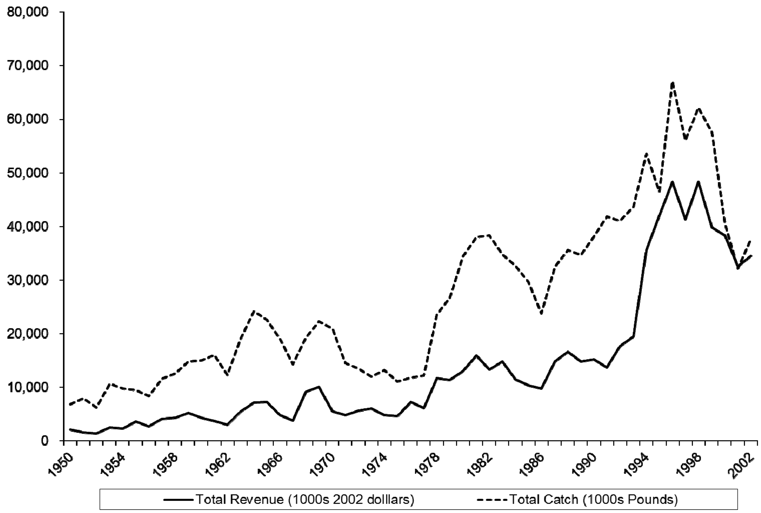
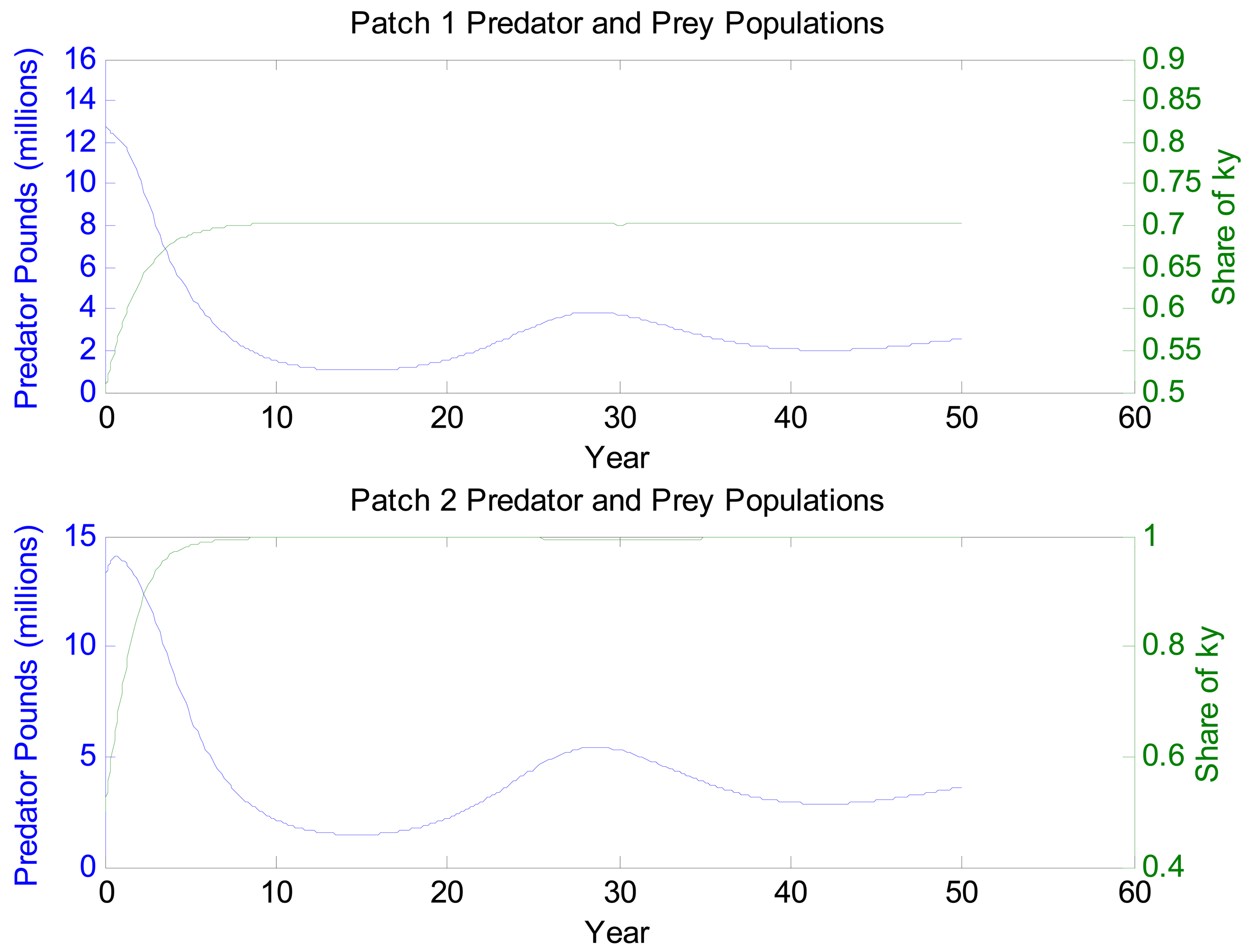
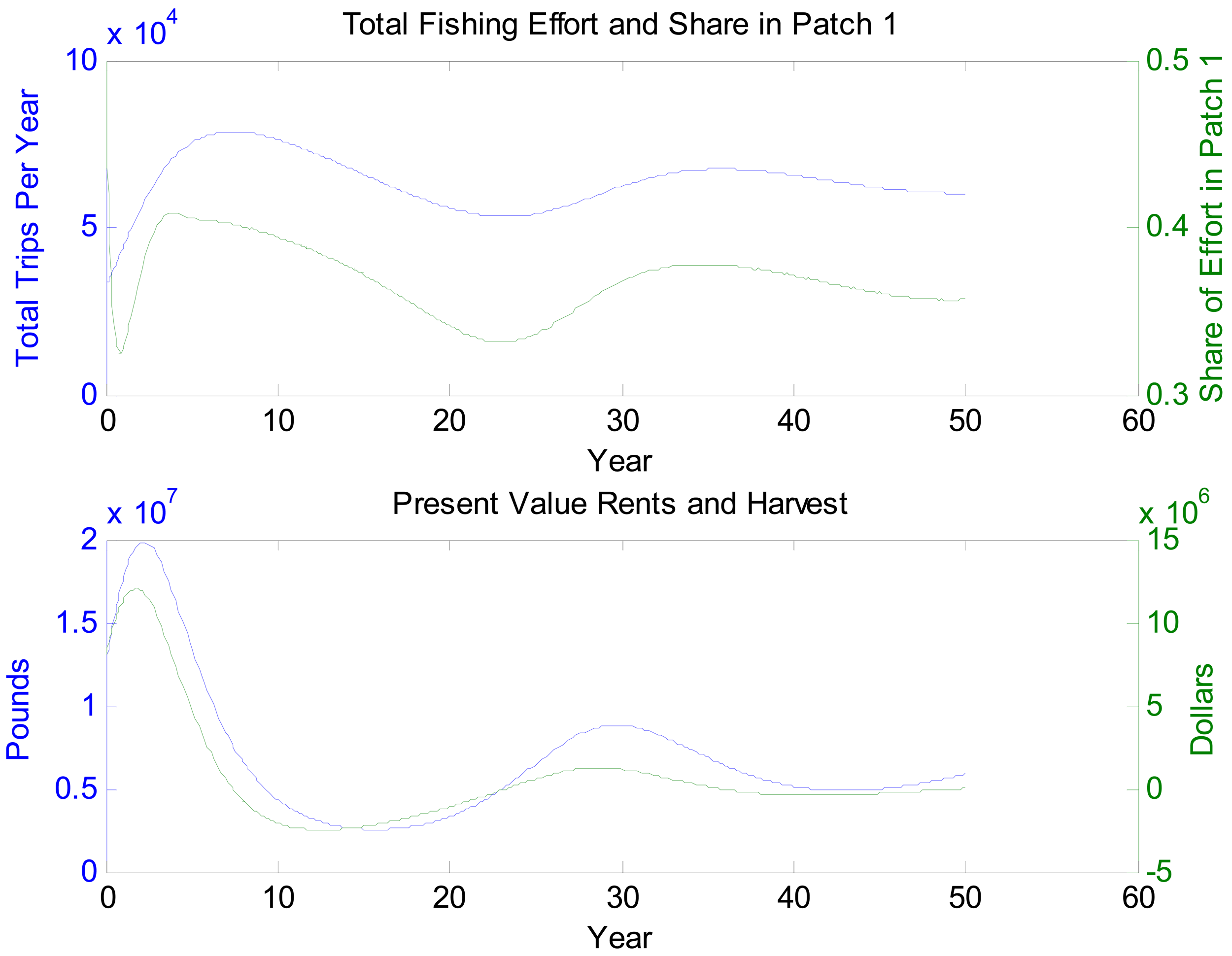
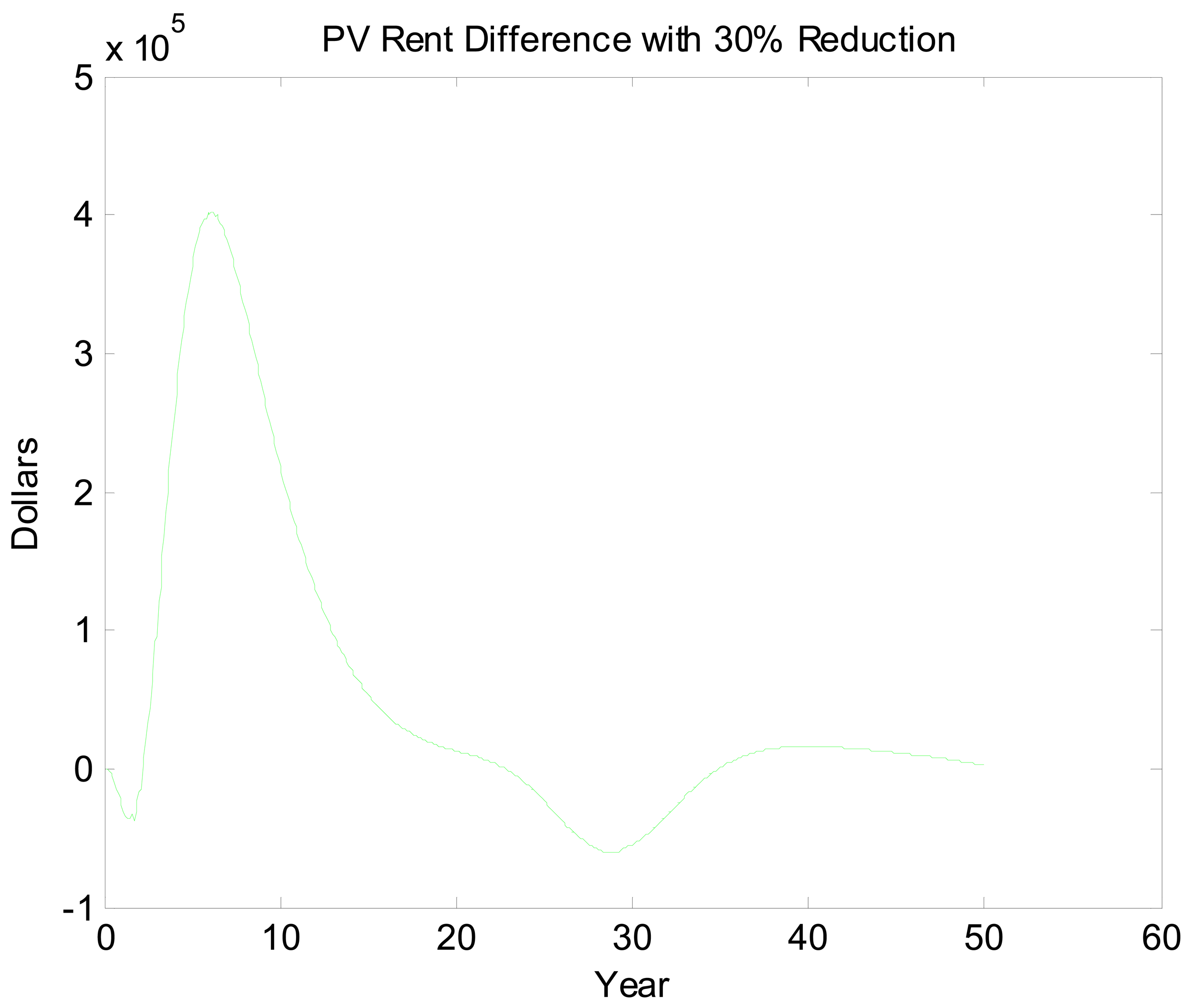
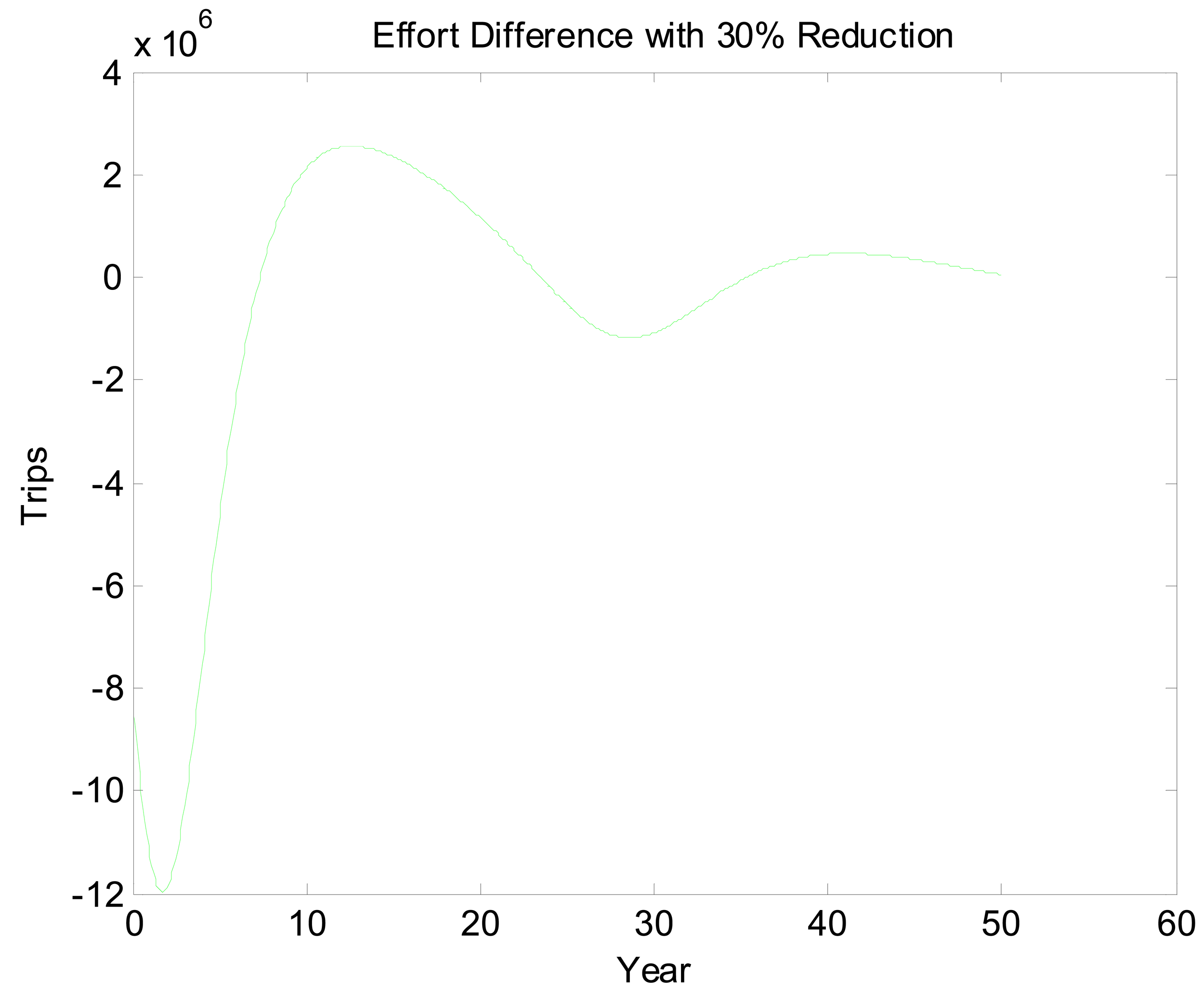
| Mu | Loadings | Implied A(0) | Total PV Rents | Change in PV | % Change | Total Catch (Million Pounds) | % Change | Total Effort (1000 s Trips) | % Change | Long-Run Catch (Million Pounds) | Long-Run Effort (1000 s Trips) |
|---|---|---|---|---|---|---|---|---|---|---|---|
| 0.05 | Baseline 30% | 0.06316 | $ 39,814,000 | 373.32 | 3,432 | 6.1384 | 65.892 | ||||
| 0.05 | Reduction | 0.06316 | $ 40,009,000 | $ 195,000 | 0.5% | 374.21 | 0.2% | 3,439 | 0.2% | 6.1513 | 66.047 |
| 0.1 | Baseline 30% | 0.12632 | $ 39,077,000 | 370.04 | 3,407 | 6.0982 | 65.354 | ||||
| 0.1 | Reduction | 0.12632 | $ 39,512,000 | $ 435,000 | 1.1% | 372.03 | 0.5% | 3,422 | 0.4% | 6.1282 | 65.702 |
| 0.2 | Baseline 30% | 0.25263 | $ 37,366,000 | 362.32 | 3,349 | 5.9975 | 64.068 | ||||
| 0.2 | Reduction | 0.25263 | $ 38,386,000 | $ 1,020,000 | 2.7% | 367.07 | 1.3% | 3,384 | 1.0% | 6.0737 | 64.911 |
| 0.4 | Baseline 30% | 0.50526 | $ 33,124,000 | 342.47 | 3,199 | 5.7003 | 60.662 | ||||
| 0.4 | Reduction | 0.50526 | $ 35,687,000 | $ 2,563,000 | 7.7% | 354.91 | 3.6% | 3,291 | 2.9% | 5.9303 | 62.93 |
| 0.6 | Baseline 30% | 0.75789 | $ 28,043,000 | 317.32 | 3,007 | 5.245 | 56.223 | ||||
| 0.6 | Reduction | 0.75789 | $ 32,459,000 | $ 4,416,000 | 15.7% | 339.86 | 7.1% | 3,176 | 5.6% | 5.7303 | 60.415 |
| 0.8 | Baseline 30% | 1.01053 | $ 22,597,000 | 288.22 | 2,780 | 4.647 | 51.125 | ||||
| 0.8 | Reduction | 1.01053 | $ 28,813,000 | $ 6,216,000 | 27.5% | 322.14 | 11.8% | 3,039 | 9.3% | 5.4585 | 57.382 |
| 0.9 | Baseline 30% | 1.13684 | $ 19,930,000 | 272.84 | 2,654 | 4.3554 | 48.563 | ||||
| 0.9 | Reduction | 1.13684 | $ 26,872,000 | $ 6,942,000 | 34.8% | 312.37 | 14.5% | 2,963 | 11.6% | 5.291 | 55.691 |
| 1 | Baseline 30% | 1.26316 | $ 17,383,000 | 257.15 | 2,523 | 4.128 | 46.043 | ||||
| 1 | Reduction | 1.26316 | $ 24,888,000 | $ 7,505,000 | 43.2% | 302.10 | 17.5% | 2,883 | 14.2% | 5.1022 | 53.906 |
Note: Assumes all other parameter values fixed at medium levels and 2.5% discount rate. Totals are totaled over 50-year simulation. Long-run values are average per year over the last two years of each simulation.
| c+ Delta | Loadings | Total PV Rents | Change in PV | % Change | Total Catch (Million Pounds) | % Change | Total Effort (1000s Trips) | % Change | Long-Run Catch (Million Pounds) | Long-Run Effort (1000s Trips) |
|---|---|---|---|---|---|---|---|---|---|---|
| 125 | Baseline 30% | $44,461,000 | 226.01 | 3,370 | 4.402 | 74.165 | ||||
| 125 | Reduction | $47,019,000 | $2,558,000 | 5.8% | 234.22 | 3.6% | 3,464 | 2.8% | 4.3475 | 76.058 |
| 175 | Baseline 30% | $38,263,000 | 275.49 | 3,324 | 3.1556 | 66.856 | ||||
| 175 | Reduction | $40,784,000 | $2,521,000 | 6.6% | 285.22 | 3.5% | 3,415 | 2.8% | 3.3185 | 68.759 |
| 225 | Baseline 30% | $33,883,000 | 325.59 | 3,228 | 4.9711 | 61.197 | ||||
| 225 | Reduction | $36,456,000 | $2,573,000 | 7.6% | 337.45 | 3.6% | 3,319 | 2.8% | 5.2012 | 63.44 |
| 240.45 | Baseline 30% | $33,124,000 | 342.47 | 3,199 | 5.7003 | 60.662 | ||||
| 240.45 | Reduction | $35,687,000 | $2,563,000 | 7.7% | 354.91 | 3.6% | 3,291 | 2.9% | 5.9303 | 62.93 |
| 275 | Baseline 30% | $31,919,000 | 381.04 | 3,141 | 7.1297 | 60.614 | ||||
| 275 | Reduction | $34,422,000 | $2,503,000 | 7.8% | 394.59 | 3.6% | 3,233 | 2.9% | 7.3491 | 62.809 |
| 325 | Baseline 30% | $30,348,000 | 435.09 | 3,068 | 8.4142 | 60.876 | ||||
| 325 | Reduction | $32,747,000 | $2,399,000 | 7.9% | 450.10 | 3.4% | 3,159 | 3.0% | 8.6546 | 62.903 |
| 375 | Baseline 30% | $28,516,000 | 485.16 | 3,000 | 9.2333 | 60.189 | ||||
| 375 | Reduction | $30,831,000 | $2,315,000 | 8.1% | 501.63 | 3.4% | 3,089 | 3.0% | 9.5265 | 62.14 |
Note: Assumes all other parameter values fixed at medium levels and 2.5% discount rate. Totals are totaled over 50-year simulation. Long-run values are average per year over the last two years of each simulation.
| Gamma | Loadings | Total PV Rents | Change in PV | % Change | Total Catch (Million Pounds) | % Change | Total Effort (1000 s Trips) | % Change | Long-Run Catch (Million Pounds) | Long-Run Effort (1000 s Trips) |
|---|---|---|---|---|---|---|---|---|---|---|
| 15 | Baseline | $ 91,214,000 | 405.89 | 3,093 | 6.727 | 61.687 | ||||
| 15 | 30% Reduction | $ 98,192,000 | $6,978,000 | 7.7% | 424.15 | 4.5% | 3,178 | 2.7% | 6.8454 | 63.797 |
| 30 | Baseline | $ 51,063,000 | 367.17 | 3,175 | 5.5887 | 65.006 | ||||
| 30 | 30% Reduction | $ 54,812,000 | $3,749,000 | 7.3% | 380.91 | 3.7% | 3,265 | 2.8% | 5.837 | 67 |
| 40 | Baseline | $ 37,768,000 | 348.69 | 3,199 | 5.2503 | 62.005 | ||||
| 40 | 30% Reduction | $ 40,659,000 | $2,891,000 | 7.7% | 361.49 | 3.7% | 3,290 | 2.8% | 5.4859 | 64.2 |
| 45.37 | Baseline | $ 33,124,000 | 342.47 | 3,199 | 5.7003 | 60.662 | ||||
| 45.37 | 30% Reduction | $ 35,687,000 | $2,563,000 | 7.7% | 354.91 | 3.6% | 3,291 | 2.9% | 5.9303 | 62.93 |
| 50 | Baseline | $ 30,242,000 | 339.45 | 3,197 | 6.2566 | 60.451 | ||||
| 50 | 30% Reduction | $ 32,573,000 | $2,331,000 | 7.7% | 351.64 | 3.6% | 3,290 | 2.9% | 6.4771 | 62.74 |
| 60 | Baseline | $ 26,273,000 | 337.93 | 3,198 | 7.0963 | 62.921 | ||||
| 60 | 30% Reduction | $ 28,205,000 | $1,932,000 | 7.4% | 349.62 | 3.5% | 3,292 | 2.9% | 7.2763 | 65.112 |
| 75 | Baseline | $ 21,874,000 | 336.26 | 3,218 | 6.2273 | 66.248 | ||||
| 75 | 30% Reduction | $ 23,375,000 | $1,501,000 | 6.9% | 347.28 | 3.3% | 3,311 | 2.9% | 6.3746 | 68.199 |
| 100 | Baseline | $ 15,583,000 | 326.84 | 3,230 | 5.362 | 60.791 | ||||
| 100 | 30% Reduction | $ 16,682,000 | $1,099,000 | 7.1% | 337.20 | 3.2% | 3,323 | 2.9% | 5.5766 | 62.722 |
| 150 | Baseline | $ 11,319,000 | 325.53 | 3,237 | 6.3249 | 66.844 | ||||
| 150 | 30% Reduction | $ 12,100,000 | $ 781,000 | 6.9% | 335.73 | 3.1% | 3,331 | 2.9% | 6.4685 | 69.173 |
| 225 | Baseline | $ 7,594,000 | 320.80 | 3,235 | 6.8168 | 63.601 | ||||
| 225 | 30% Reduction | $ 8,167,000 | $ 573,000 | 7.5% | 330.56 | 3.0% | 3,327 | 2.8% | 7.2096 | 66.032 |
| 350 | Baseline | $ 5,017,000 | 318.93 | 3,246 | 6.6801 | 64.286 | ||||
| 350 | 30% Reduction | $ 5,453,000 | $ 436,000 | 8.7% | 328.35 | 3.0% | 3,335 | 2.8% | 7.1528 | 66.775 |
Note: Assumes all other parameter values fixed at medium levels and 2.5% discount rate. Totals are totaled over 50-year simulation. Long-run values are average per year over the last two years of each simulation.
Acknowledgments
Financial support for this projected was provided by NSF Grant # SES-0083327 and NOAA's Center for Sponsored Coastal Ocean Research Grant # NA05NOS4781197. The authors would like to thank Kerry Smith, David Finnoff, Lisa Eby, Tom Miller, Joe Ramus, Mike Orbach, Ken Reckhow, Bob Christian, Craig Stow, Doug Lipton, and Lynn Maguire for helpful comments and suggestions, Sam Cunningham for research assistance, and thank David Eggleston and Sean McKenna for access to unpublished data and reports.
Appendix A. Summary of parameterization
| Equation(s) | Parameter Name | Value | Source/Comment |
|---|---|---|---|
| 1 | Lbar | 1.2 | From Neuse TMDL (adjusted down from 1.3 to account some for stock in the system) |
| 1 | omega | 0.95 | A slow decay rate based on persistence of nutrients |
| 2 | mu | 0.4 | Borsuk, Stow, and Reckhow (2004b) |
| 3, 4, 5 | rx | 0.75 | Eggleston et al. (2004) |
| 3, 4, 5 | kx | 25.85 | Eggleston et al. (2004). Carrying capacity scaled down to reflect the size of the fishery in the Neuse River and Pamlico Sound only |
| 3, 4, 5 | alpha | 0.37 | Backed out using Excel's nonlinear solver and imposing the steady-state condition in patch 1 (or 2) with no hypoxia |
| 4, 5 | phi | 50 | Scale intuition based on relative carrying capacities |
| 4, 5 | chsi | 0.5 | Allows for a wide range of responsiveness (and the potential for collapses in patch 1), less than or equal to corresponding rx to prevent negative populations |
| 6, 7 | beta | 0.001 | Chosen to scale predation such that abs(beta*kx) < ry |
| 6, 7 | ry | 0.97 | Clams are assumed fast growing (they are k-limited and not r-limited). Magnitude based on the survival regression in Borsuk, Powers and Peterson (2002) using minimum growth rate necessary to prevent population collapse under worst in-sample dissolved oxygen |
| 7 | rho | 0.79 | Computed elasticity from Borsuk, Higdon, Stow, and Reckhow (2001) combined with Borsuk, Powers and Peterson (2002) |
| 11, 12, 16, 17 | p | 0.87 | Mean real price (weighted avg aggregated across hard, soft, and peeler, 1998–2002). In 2002 dollars using CPI Size D South |
| 11, 12, 16, 17 | c + delta | 240.45 | Rhodes, Lipton, and Shabman (2001) converted to 2002 dollars |
| 12, 17 | gamma | 45.37 | Estimated jointly with 1-period ahead forecasts on catch per trip data (1982–2002) converting pots to trips and excluding 1994–1999 due to overreporting of pots. Pots converted to trips based on 2000–2002 trip data. |
| 13, 14 | theta | 0.4 | Smith and Wilen (2003) |
| 15 | q | 0.00003 | Using parms from Eggleston et al. (2004) calibrated to total catch across time and pattern of catch. |
| Neuse share of total NC | 0.35 | Share of the fishery in the Neuse River and Estuary + the Pamlico Sound | |
| Initial Conditions | |||
| 1 | N(0) | 1.26 | Loadings divided by w (start off at steady-state stock) |
| 2 | A(0) | 0.51 | Algae starts in a steady-state. |
| 4, 5 | X_1(0) = X_2(0) | 12.92 | 1/2 of kx (bundled to pop. Parameters) |
| 6, 7 | Y_1(0) = Y_2(0) | 0.50 | 1/2 of y carrying capacity |
| 14 | pi_1(0) | 0.5 | Initial effort allocated uniformly over space. |
| 17 | E(0) | 32,077 | 35% of effort in the fishery (mean over 2000–2002) |
References and Notes
- National Research Council. Clean Coastal Waters: Understanding and Reducing the Effects of Nutrient Pollution; National Academy Press: Washington, DC, USA, 2000. [Google Scholar]
- Craig, J.K.; Crowder, L.B. Hypoxia-induced habitat shifts and energetic consequences in atlantic croaker and brown shrimp on the Gulf of Mexico shelf. Mar. Ecol. Prog. Ser. 2005, 294, 79–94. [Google Scholar]
- Craig, J.K.; Crowder, L.B.; Gray, C.D.; McDaniel, C.J.; Henwood, T.A.; Hanifen, J.E. Ecological effects of hypoxia on fish, sea turtles, and marine mammals in the Northwestern Gulf of Mexico. In Coastal Hypoxia: Consequences for Living Resources and Ecosystems; Rabalais, N.N., Turner, R.E., Eds.; American Geophysical Union, Coastal and Estuarine Studies: Washington, DC, USA, 2001; pp. 269–292. [Google Scholar]
- Peterson, C.H.; Summerson, H.C.; Thomson, E.; Lenihan, H.S.; Grabowski, J.; Manning, L.; Micheli, F.; Johnson, G. Synthesis of linkages between benthic and fish communities as a key to protecting essential fish habitat. Bull. Mar. Sci. 2000, 66, 759–774. [Google Scholar]
- Baird, D.; Christian, R.R.; Peterson, C.H.; Johnson, G.A. Consequences of hypoxia on estuarine ecosystem function: Energy diversion from consumers to microbes. Ecol. Appl. 2004, 14, 805–822. [Google Scholar]
- Caddy, J.F. Towards a comparative evaluation of human impacts on fishery ecosystems of enclosed and semi-enclosed seas. Rev. Fish. Sci. 1993, 1, 57–95. [Google Scholar]
- National Research Council. Assessing the TMDL Approach to Water Quality Management; National Academy Press: Washington, DC, USA, 2001. [Google Scholar]
- Phase II of the Total Maximum Daily Load for Total Nitrogen to the Neuse River Estuary, North Carolina; North Carolina Department of Environment and Natural Resources Division of Water Quality: Raleigh, NC, USA, 2001.
- Paerl, H.W.; Pinckney, J.L.; Fear, J.M.; Peierls, B.L. Ecosystem responses to internal and watershed organic matter loading: Consequences for hypoxia in the eutrophying Neuse River Estuary, North Carolina, USA. Mar. Ecol. Prog. Ser. 1998, 166, 17–25. [Google Scholar]
- Eby, L.A.; Crowder, L.B. Hypoxia-based habitat compression in the Neuse River Estuary: Context-dependent shifts in behavioral avoidance thresholds. Can. J. Fish. Aquat. Sci. 2002, 59, 952–965. [Google Scholar]
- Eby, L.A.; Crowder, L.B. Effects of hypoxic disturbances on an estuarine nekton assemblage across multiple scales. Estuaries 2004, 27, 342–351. [Google Scholar]
- Powers, S.P.; Peterson, C.H.; Sullivan, E.; Powers, M.J.; Vandenburgh, E.; Bishop, M.; Christian, R.; Buzzelli, C.P. Effects of eutrophication on bottom habitat and prey resources of demersal fishes. Mar. Ecol. Prog. Ser. 2005, 302, 233–243. [Google Scholar]
- Eby, L.A.; Crowder, L.B.; McClellan, C.M.; Peterson, C.H.; Powers, M.J. Habitat degradation from intermittent hypoxia: Impacts on demersal fishes. Mar. Ecol. Prog. Ser. 2005, 291, 249–261. [Google Scholar]
- Miller, T.J. Incorporating space into models of the Chesapeake Bay blue crab population. Bull. Mar. Sci. 2003, 72, 567–588. [Google Scholar]
- Etherington, L.L.; Eggleston, D.B. Large-scale blue crab recruitment: Linking postlarval transport, post-settlement planktonic dispersal, and multiple nursery habitats. Mar. Ecol. Prog. Ser. 2000, 204, 179–198. [Google Scholar]
- Blue Crab. Chesapeake Bay Program Website. Available online: http://www.chesapeakebay.net/info/blue_crab.cfm (accessed on 9 April 2004).
- Selberg, C.D.; Eby, L.A.; Crowder, L.B. Hypoxia in the Neuse River Estuary: Responses of blue crabs and crabbers. N. Am. J. Fish. Manag. 2001, 21, 358–366. [Google Scholar]
- NOAA Fisheries. NOAA Fisheries Commercial Landings Data Website. Available online: http://www.st.nmfs.gov/st1/commercial/landings/annual_landings.html (accessed on 12 September 2004).
- Burgess, C.C.; Bianchi, A.J. An Economic Profile Analysis of the Commercial Fishing Industry of North Carolina Including Profiles for State-Managed Species; North Carolina Department of Environment and Natural Resources, Division of Marine Fisheries, License and Statistics Section: Morehead City, NC, USA, 2004. [Google Scholar]
- Draft 3 North Carolina Fishery Management Plan: Blue Crab, 2004; North Carolina Department of Environment and Natural Resources, Division of Marine Fisheries: Raleigh, NC, USA, 2004.
- Upadhyaya, K.P.; Larson, J.B.; F.G. Mixon, J. The economic impact of environmental regulation on the blue crab industry. Int. J. Soc. Econ. 2002, 29, 538–546. [Google Scholar]
- Dasgupta, P.; Maler, K.G. The economics of non-convex ecosystems: Introduction. Environ. Res. Econ. 2003, 26, 499–525. [Google Scholar]
- Brock, W.A.; Starrett, D. Managing systems with non-convex positive feedback. Environ. Res. Econ. 2003, 26, 575–602. [Google Scholar]
- Arrow, K.J.; Dasgupta, P.; Maler, K.G. Evaluating projects and assessing sustainable development in imperfect economies. Environ. Res. Econ. 2003, 26, 647–685. [Google Scholar]
- Geyer, W.R.; Morris, J.T.; Prahl, F.G.; Jay, D.A. Interaction between physical processes and ecosystem structure: A comparative approach. In Estuarine Science: A Synthetic Approach to Research and Practice; Hobbie, J.E., Ed.; Island Press: Washington, DC, USA, 2000. [Google Scholar]
- Blue Crab Life Cycle. The Blue Crab Archives Website. Available online: http://www.bluecrab.info/lifecycle.html (accessed on 24 July 2011).
- Ragozin, D.L.; Brown, G. Harvest policies and nonmarket valuation in a predator-prey system. J. Environ. Econ. Manag. 1985, 12, 155–168. [Google Scholar]
- Wilen, J.; Brown, G. Optimal recovery paths for perturbations of trophic level bioeconomic systems. J. Environ. Econ. Manag. 1986, 13, 225–234. [Google Scholar]
- Kahn, J.R.; Kemp, W.M. Economic losses associated with the degradation of an ecosystem: The case of submerged aquatic vegetation in chesapeake bay. J. Environ. Econ. Manag. 1985, 12, 246–263. [Google Scholar]
- McConnell, K.E.; Strand, I.E. Benefits from commercial fisheries when demand and supply depend on water quality. J. Environ. Econ. Manag. 1989, 17, 284–292. [Google Scholar]
- Swallow, S.K. Depletion of the environmental basis for renewable resources: The economics of interdependent renewable and nonrenewable resources. J. Environ. Econ. Manag. 1990, 19, 281–296. [Google Scholar]
- Barbier, E.B.; Strand, I.E. Valuing mangrove-fishery linkages: A case study of Campeche, Mexico. Environ. Res. Econ. 1998, 12, 151–166. [Google Scholar]
- Knowler, D.; Barbier, E.B.; Strand, I.E. An open-access model of fisheries and nutrient enrichment in the Black Sea. Mar. Res. Econ. 2001, 16, 195–217. [Google Scholar]
- Sanchirico, J.N.; Wilen, J.E. Bioeconomics of spatial exploitation in a patchy environment. J. Environ. Econ. Manag. 1999, 37, 129–150. [Google Scholar]
- Taylor, D.L.; Eggleston, D.B. Effects of hypoxia on an estuarine predator-prey interaction: Foraging behavior and mutual interference in the blue crab callnectes sapidus and the infaunal clam prey mya arenaria. Mar. Ecol. Prog. Ser. 2000, 196, 221–237. [Google Scholar]
- Smith, M.D. Two econometric approaches for predicting the spatial behavior of renewable resource harvesters. Land Econ. 2002, 78, 522–538. [Google Scholar]
- Smith, M.D.; Wilen, J.E. Economic impacts of marine reserves: The importance of spatial behavior. J. Environ. Econ. Manag. 2003, 46, 183–206. [Google Scholar]
- Smith, V.L. Economics of production from natural resources. Am. Econ. Rev. 1968, 58, 409–431. [Google Scholar]
- Smith, V.L. On models of commercial fishing. J. Polit. Econ. 1969, 77, 181–198. [Google Scholar]
- Wilen, J.E. Common Property Resources and the Dynamics of Overexplotiation: The Case of the North Pacific Fur Seal; Department of Economics Resources Paper No. 3; University of British Columbia: Vancouver, Canada, 1976. [Google Scholar]
- Gordon, H.S. Economic theory of a common property resource: The fishery. J. Polit. Econ. 1954, 62, 124–142. [Google Scholar]
- Bockstael, N.E.; Opaluch, J.J. Discrete modelling of supply response under uncertainty: The case of the fishery. J. Environ. Econ. Manag. 1983, 10, 125–137. [Google Scholar]
- Smith, M.D. State dependence and heterogeneity in fishing location choice. J. Environ. Econ. Manag. 2005, 50, 319–340. [Google Scholar]
- Borsuk, M.E.; Stow, C.A.; Reckhow, K.H. Integrated approach to tmdl development for the Neuse River Estuary using a Bayesian probability network model (NEU-BERN). J. Water Res. Plan. Manag. 2003, 129, 271–282. [Google Scholar]
- Borsuk, M.E.; Stow, C.A.; Reckhow, K.H. A Bayesian network of eutrophication models for synthesis, prediction, and uncertainty analysis. Ecol. Model. 2004, 173, 219–239. [Google Scholar]
- Stow, C.A.; Borsuk, M.E. Assessing TMDL effectiveness using flow-adjusted concentrations: A case study of the Neuse River Estuary, NC. Environ. Sci. Technol. 2003, 37, 2043–2050. [Google Scholar]
- Borsuk, M.E.; Stow, C.A.; Reckhow, K.H. The confounding effect of flow on estuarine response to nitrogen loading. J. Environ. Eng. 2004, 130, 605–614. [Google Scholar]
- Borsuk, M.E.; Stow, C.A.; Luettich, R.A.; Paerl, H.W.; Pinckney, J.L. Modeling oxygen dynamics in an intermittently stratified estuary: Estimation of process rates using field data. Estuar. Coast. Shelf Sci. 2001, 52, 33–49. [Google Scholar]
- Borsuk, M.E.; Stow, C.A.; Higdon, D.; Reckhow, K.H. A Bayesian hierarchical model to predict benthic oxygen demand from organic matter loading in estuaries and coastal zones. Ecol. Model. 2001, 143, 165–181. [Google Scholar]
- Borsuk, M.E.; Powers, S.P.; Peterson, C.H. A survival-based model of the effects of bottom-water hypoxia on the density of an estuarine clam (Macoma balthica). Can. J. Fish. Aquat. Sci. 2002, 59, 1266–1274. [Google Scholar]
- Eggleston, D.B.; Johnson, E.G.; Hightower, J.E. Population Dynamics and Stock Assessment of the Blue Crab in North Carolina; Final Report for Contracts 99-FEG-10 and 00-FEG-11 for the North Carolina Fishery Resource Grant Program, North Carolina Sea Grant, and the North Carolina Department of Environmental Health and Natural Resources, Division of Marine Fisheries: Raleigh, NC, USA, 2004. [Google Scholar]
- Rhodes, A.; Lipton, D.; Shabman, L. A socio-economic profile of the Chesapeake Bay commercial blue crab fishery; Virginia Commonwealth University: Richmond, VA, USA, Unpublished Technical Report; 2001. [Google Scholar]
- Smith, M.D.; Wilen, J.E. Marine reserves with endogenous ports: Empirical bioeconomics of the California sea urchin fishery. Mar. Res. Econ. 2004, 19, 85–112. [Google Scholar]
- Kaoru, Y.; Smith, V.K.; Liu, J.L. Using random utility models to estimate the recreational value of estuarine resources. Am. J. Agric. Econ. 1995, 77, 141–151. [Google Scholar]
- Mansfield, C.; Smith, V.K. Tradeoffs at the trough: TMDLs and the evolving status of us water quality policy. In Recent Advances in Environmental Economics; List, J.A., De Zeeuw, A., Eds.; Edward Elgar: Northhampton, MA, USA, 2002. [Google Scholar]
- Phaneuf, D.J. A random utility model for toal maximum daily loads: Estimating the benefits of watershed-based ambient water quality improvements. Water Resour. Res. 2002, 38, 1–11. [Google Scholar]
- Smith, V.K.; Schwabe, K.A.; Mansfield, C. Does nature limit environmental federalism? In Environmental and Public Economics: Essays in Honor of Wallace E. Oates; Panagariya, A., Portney, P.R., Schwab, R.M., Eds.; Edward Elgar: Northhampton, MA, USA, 1999. [Google Scholar]
- Freeman, A. Valuing environmental resources under alternative management regimes. Ecol. Econ. 1991, 3, 247–256. [Google Scholar]
- Krutilla, J.V.; Eckstein, O. Multiple Purpose River Development; The Johns Hopkins Press for Resources for the Future: Baltimore, MD, USA, 1958. [Google Scholar]
- Smith, V.K. Krutilla's legacy: Twenty-first-century challenges for environmental economics. Am. J. Agric. Econ. 2004, 86, 1167–1178. [Google Scholar]
- McConnell, K.E.; Sutinen, J.G. Bioeconomic models of marine recreational fishing. J. Environ. Econ. Manag. 1979, 6, 127–139. [Google Scholar]
- Bishop, R.C.; Samples, K.C. Sport and commercial fishing conflicts: A theoretical analysis. J. Environ. Econ. Manag. 1980, 7, 220–233. [Google Scholar]
- Copes, P.; Knetsch, J.L. Recreational fisheries analysis: Management modes and benefit implications. Can. J. Fish. Aquat. Sci. 1981, 38, 559–570. [Google Scholar]
- Johnson, R.N.; Libecap, G.D. Contracting problems and regulation: The case of the fishery. Am. Econ. Rev. 1982, 72, 1005–1022. [Google Scholar]
- Hammitt, J.K. Economic implications of hormesis. Hum. Exp. Toxicol. 2004, 23, 267–278. [Google Scholar]
- Provencher, B.; Burt, O. The externalities associated with the common property exploitation of groundwater. J. Environ. Econ. Manag. 1993, 24, 139–158. [Google Scholar]
- Maler, K.G.; Xepapadeas, A.; Zeeuw, A.D. The economics of shallow lakes. Environ. Res. Econ. 2003, 26, 603–624. [Google Scholar]
- Court, R.H. Efficient estimation of the reduced form from incomplete econometric models. Rev. Econ. Stud. 1973, 40, 411–417. [Google Scholar]
© 2011 by the authors; licensee MDPI, Basel, Switzerland. This article is an open access article distributed under the terms and conditions of the Creative Commons Attribution license (http://creativecommons.org/licenses/by/3.0/).
Share and Cite
Smith, M.D.; Crowder, L.B. Valuing Ecosystem Services with Fishery Rents: A Lumped-Parameter Approach to Hypoxia in the Neuse River Estuary. Sustainability 2011, 3, 2229-2267. https://doi.org/10.3390/su3112229
Smith MD, Crowder LB. Valuing Ecosystem Services with Fishery Rents: A Lumped-Parameter Approach to Hypoxia in the Neuse River Estuary. Sustainability. 2011; 3(11):2229-2267. https://doi.org/10.3390/su3112229
Chicago/Turabian StyleSmith, Martin D., and Larry B. Crowder. 2011. "Valuing Ecosystem Services with Fishery Rents: A Lumped-Parameter Approach to Hypoxia in the Neuse River Estuary" Sustainability 3, no. 11: 2229-2267. https://doi.org/10.3390/su3112229