The Architecture and Measurement of an Ecosystem Services Index

Abstract

This paper discusses the construction of an ecosystem services index (ESI) and the respective roles of ecology and economics in that effort. It extends the concept of an ESI, analogous to Gross Domestic Product, to other analogous indices, including an ecosystem price or value index, and a net ESI that accounts for interactions between ecosystem stocks and service flows. A central aim of this paper is to account for services in an economically and ecologically defensible manner. It thus also discusses the connection between ecological models and economic models in the construction of ecosystem services indices, the former on the quantity side and the latter on the price/value side of the index.

1. Introduction

Joint models of ecosystems and of economic activity have played an important role in environmental policy since the seminal work of Kneese and Bower [1]. The interface between ecology and the economy remains a priority for decision making and a challenge for the sciences. Separately, ecology and economics have advanced much faster than the integrated methods necessary for real descriptive and predictive power. This paper confronts the challenge of “real descriptive and predictive power” by drawing on ecological principles, economic and biophysical data, and the economic theory of index numbers to propose indicators of ecologically derived well-being that can be used in policy analysis and interdisciplinary models.

Capturing nature’s production of goods and services in a comprehensive way is a tall order. Ecological systems are complex, with a nearly uncountable number of components interacting non-linearly. Is it realistic to think we can capture such a complex system in a practical index? Not if the goal is a comprehensive knowledge of ecological production. But accounting systems serve narrower ends. They provide a rough, but valuable, guide to the more complex systems they describe. The conventional economy is also a complex, multi-dimensional, and non-linear system. We do not look to Gross Domestic Product (GDP) or other economic indices for the entire truth about our economies. Rather, we look to them as important signals of our welfare and progress or decline, and they are useful for that purpose. Nature’s non-market contributions to our wellbeing deserve a similar set of signals.

In particular, the paper discusses the respective roles of ecology and economics in the construction of an ecosystem services index (ESI), proposed by Boyd and Banzhaf [2] (see also [3,4,5]). Any index, whether it is an ESI or something more familiar, such as GDP, is meant to aggregate and summarize a collection of disparate elements. An ESI is a measure of quantity that relates to, but does not measure directly, the total value of nature. As proposed by Boyd and Banzhaf, an ESI measures the value of “final” ecosystem services, i.e., the final outputs of nature, whether enjoyed directly by people or used by people as inputs, in combination with labor and man-made capital, to produce goods. Such a stand-alone index of ecosystem services would serve as a useful government performance measure and a yardstick of gains and losses to environment-related well-being. By limiting it only to the final non-market services, it could also be combined with GDP to form a measure of Green GDP [6,7,8,9,10,11,12,13,14,15].

We begin by discussing the architecture of an ecosystem services index, emphasizing three aspects. First, ecosystem services must be measured and expressed in defined, standardized units. Markets tend to standardize units of consumption for conventional goods and services. Recognizable units aid marketing, bargaining, and the resolution of disputes. By contrast, ecological outputs are often public goods, not associated with markets, and thus tend to lack standardized measures of output.

Second, there is a fundamental distinction between services and the values of those services, a distinction which must be taken into consideration when generating aggregate indices. Insights from the “index number problem” suggest that to facilitate comparisons across time and space, ecosystem services must be aggregated using a constant set of value weights. By the same token, the ESI has a dual index, analogous to a price index, which can measure the changing value of a fixed bundle of ecosystem services to people or the relative value of providing services at different places. The indices must be defined jointly, and each has a role to play in informing policy. Conflating these roles has been one source of confusion in the literature.

Third, ecosystem service flows depend on biophysical stocks. These stocks are the biological and physical assets that produce ecosystem services. They include clean air, water, habitat, and biotic populations. Like the services they generate, they typically are not defined or valued by markets—in fact, the only way to value these stocks is to value the flows of goods and services they generate. Ecosystem stocks can be thought of as claims on future ecosystem service flows. Accordingly, an index should measure not only current flows but also gains or losses (depletion) of stock assets that affect future service flows. We extend our concept of an ESI to such stock-flow concerns, introducing the concept of a net ESI, analogous to net GDP. The distinction between ecosystem services and ecological stocks is important not only to the formal construction of an index but also to the measurement of environmental outcomes and interactions between economic and ecological science.

Drawing on these three aspects of an ESI’s architecture, we then reflect on the respective roles of ecology and economics in its construction, and the ways they must come together to fruitfully measure ecosystem services. First, our emphasis on measurable units reflects the point at which they most connect: the measures of physical ecosystem services must synch up with measures of their respective values. Second, the economic theory of stock-flow interactions underlying a net ESI requires a particular type of predictive ecology.

Naturally, an ESI requires both economic and ecological content and analysis. Accordingly, a further goal of this paper is to assess the utility of existing ecological indices and indicators in the construction of an index such as ours. In economic terms, most theoretical and empirical ecology is geared toward the depiction of ecological asset qualities and interdependencies between ecological assets. Accordingly, ecological models and indicator systems play the central role in the assessment of stock effects. However, biophysical science is often not geared toward the assessment of service flows arising from those assets. Economics plays an important role in helping define measures of these service flows and ways to weight them. Our architecture highlights the complementary roles of ecology and economics in resolving these measurement issues.

1.1. Why Construct an Ecosystem Services Index?

The question of why to construct an ESI has three sub-components. First, why is a measure of ecological conditions needed? Second, why measure ecological conditions as they relate to economic benefits or services? And third, why construct an index to measure these services? With regard to the first question, indicators of ecological condition may have several purposes. Most simply, they may help us to satisfy our natural desire to evaluate the state of things by comparing differences across space and by tracking changes over time. In this way, indicators help us to answer the question: “how are we doing ecologically?” Accordingly, they also may help identify problems on the horizon or help us evaluate the success of past policies, if only indirectly. By the same token, measurement of ecosystem services in a manner consistent with the national accounts will ultimately help enrich national accounting measures such as GDP. Finally, in joint models of ecological and economic systems, indicators of ecological condition play a crucial role in the feedback between the two systems.

The second part of the question—why measure the economic characteristics of ecological conditions—is obvious to economists but may not be to others. We emphasize economic indicators of ecosystem services for two broad reasons: one philosophical, one pragmatic. As a matter of philosophy, economists believe that the objective of social policy is to maximize as best as possible human well-being. When we measure ecological conditions alone it is certainly far better than doing nothing, but it neglects deeper inquiry into what is socially beneficial about ecological systems. The second reason to assess human services provided by the natural environment is that it illuminates tradeoffs and the setting of priorities. Indicators of pure ecological condition do not help a decision-maker forced to choose between conflicting interventions. To say that better ecological conditions are better for society is true but unhelpful. In practice, decision-makers struggle with much more difficult questions, such as which ecological conditions are better than others? The economist’s answer is that measures of social well-being—the services provided by nature—should guide the choice.

It should be emphasized, however, that any economic assessment of ecological benefits must be built on a foundation of biophysical analysis. The economist’s role is to evaluate the consequences of an ecological change to social well-being. Economists rely on the biophysical sciences to describe those changes. Without biophysical assessment there can be no economic assessment. Accordingly, ecological benefit analysis is inherently integrative, demanding cross-disciplinary understanding, if not collaboration. The ESI architecture embodies that principle.

The third question is why capture ecosystem services via an index? An index is designed to aggregate a broad range of services into a simple measure, with breadth referring both to the type of services and their spatial and temporal distribution. The issues we discuss apply to a national ESI as directly as they apply to an ESI at other meaningful scales (e.g., watersheds). Such aggregation and simplification can be useful to policymakers (and the public) by illuminating the big picture and by reducing a potentially vast array of signals into a smaller dimension that can be more easily processed by decision-makers. By the same token, by reducing the dimensionality of the problem in a theoretically consistent way, indices can be useful in models of the interaction between ecosystems and economic systems. For example, equilibrium or simulation models of an ecosystem and economy must constrain the dimensionality of the problem within computational limits. Creating one or a few aggregate flow(s) of services from the ecosystem to the economy is one way to do so.

2. The Architecture of an Ecosystem Services Index

Previously, we have suggested a definition of ecosystem goods and services compatible with GDP accounting [2] (see also [4,5,16,17]). This definition involves two fundamental principles. First, ecosystem goods and services are ecological commodities, measured in physical terms. They are distinct from the values people have for those services or the benefits they generate. Similarly, in GDP-type accounts, there is a corresponding distinction between quantity measures and the price measures used to weight them.

Second, ecosystem goods and services as we define them are the “final products” of natural systems. Either they are enjoyed directly by people (e.g., a natural view) or they are productively used in the creation of man-made goods (e.g., the bees used in the production of apples or almonds). Following this reasoning, we suggest the following guiding principle to identify quantity measures of ecosystem services for an ESI: they are quantities, features, or qualities of an ecosystem that represent the last link in the chain of ecological and economic production that still involves ecological factors as an input. Or, to put it in other terms, ecosystem goods and services are the biophysical quantities and qualities that are directly combined with market goods and services in firm or household production. As we argue in [2], the bees would enter an ESI, since they are combined with man-made inputs to produce agricultural outputs.

This principle puts the ecosystem on an equal footing with market inputs and outputs by identifying the point at which they come together in production. This is important because it means our definition will allow for the eventual integration of an ESI into a more comprehensive set of national accounts. Our definition of services is entirely consistent with that used in conventional income accounting, so that our ESI could be combined with conventional GDP for a measure of green GDP [18,19]. For interdisciplinary models of ecosystems and economic systems (e.g., [20,21]), the ecosystem services can be thought of as the value of “exports” from the ecosystem sector of the model to the man-made economic sector. As we discuss in this section, the analogy to GDP accounting and the so-called “index number problem” helps clarify the distinct roles to be played by an index that constructs a bundle of services and an index measuring the anthropocentric value of such a bundle of services.

Our focus on final services should not give the misimpression that intermediate ecological assets are unimportant or not valuable (see [5,16] for more discussion on this distinction). To the contrary, they are crucial for the provision of ecosystem services—just as human inputs into economic production, like labor and capital, are crucial for economic production, yet are not counted as final goods and services. However, the value of natural capital and intermediate services is embodied in the value of those final ecosystem services flows. As we further argue in this section, in the case of natural capital that provides ecosystem services over time, it is important to account for the connection between these stocks and flows.

2.1. Ecological Services, Ecological Assets

We begin by making a basic distinction between the ecosystem itself, ecosystem stocks—or ecological assets, and the services that the system of stocks provides. We denote by Q an ecosystem, which may be partitioned into a set of ecosystem components (Q₁, …, Q_j, …, Q_J), each with some physical measure of its quantity or quality. The J parts of the ecosystem may be distinguished by media, spatial location, hydrological function, or biological function (e.g., place in the foodweb). While an ecosystem is an abstraction, the Q_j are, in principle, measurable features or qualities. Ecosystem stocks can be individual Q_j, such as a quantity of water contained in a subsurface aquifer, or collections of Q_j, such as a forest composed of various tree and animal species, soils, and water resources. They can also represent the qualities of an ecosystem feature, such as the chemical composition of surface waters or diversity of species present in a given area.

The ecosystem, or ecosystem stocks into which it is decomposed, produce a set of goods and services q = (q₁, …, q_i, …, q_I) enjoyed by people. This flow of goods and services is derived from the ecosystem according to an ecological production function that is a mapping from ℝ ^J to ℝ^I:

                                   q = F(Q)                                   (1)

These goods and services are flows consumed directly by households or other economic agents, whereas the ecosystem components are stocks that are necessary inputs to the provision of the final goods and services. In some cases, the relationship represented by F( ) is likely to be highly complex and non-linear. In other cases, however, it may be trivially simple. For example, if Q_j represents the stock of bald eagles, and if households place a value on the total number of bald eagles, the stock yields an existence–value service flow q_i = Q_j.

In most modeling and policy applications, it is necessary to reduce the dimensionality of q or Q. Linear indices, such as those used in the national accounts, are a feasible approach. A linear index is merely a weighted average of its components.

Knowledge of the ecological production function F( ) is not actually necessary if the goal of measurement is only to measure the production and consumption of q in a given period. F( ) is necessary if the ESI is designed to measure the depletion (or enhancement) of future good and service flows q. The effect of current period losses or gains in ecosystem stocks or quality on future production of q is determined by F( ). F( ) is also generally necessary to the cost-benefit analysis of environmental protection, policy, and management, since the goal of such analysis is usually to translate policies that affect elements of Q into the consequences for ecosystem goods and services q. The role of depletion analysis in an ESI is discussed in more detail in section 2.5.

2.2. A Revenue Index

Consider first one particular linear aggregation: the sum of ecosystem services weighted by their marginal values or people’s marginal willingness to pay (WTP). These marginal values are analogous to prices in a market economy, and economists sometimes refer to them as “virtual prices” for non-market goods. In a market economy, prices are equal to marginal WTP, as consumers will buy a good as long as its value is higher than the price. These marginal values decline with successive purchases, until the marginal value is equal to the price, at which point purchases stop. By the same token, the marginal value of an ecosystem service is the price at which consumers would have purchased the quantity of service that actually is observed to prevail in the real world—if their income were augmented to cover the purchase. For this reason, these concepts are known as “virtual prices” and “virtual income” [22,23].

Marginal values are not the only conceivable weights, but they do reflect our anthropocentric approach to measuring services. The sum of ecosystem services weighted by marginal WTP (prices) can be thought of as a revenue index, as it represents the revenue that could be obtained by hypothetically selling all services at marginal values. The revenue index at time or place t is

                                   R^t = Σ_iq_i^tp_i^t.                                    (2)

Such an index may be a useful proxy to policymakers in a variety of settings. Suppose for example that we must choose between the protection of two wilderness areas designated by 0 and 1. Using the revenue index at each site, we might compare Σ_iq_i⁰p_i⁰ to Σ_iq_i¹p_i¹ and preserve the one with the greatest value.

However, as an aid to policymaking, the revenue index has two main problems. The first relates to the index’s reliance on marginal values. Suppose both sites are in areas with equal populations of similar incomes and tastes and where there are similar opportunities for substitution. Further suppose that site 1 offers more services in the sense that q_i¹ > q_i⁰ for all services i. This increased supply of services from site 1 would drive down their marginal values (because of diminishing marginal WTP) so that p_i¹ < p_i⁰ for all i. Depending on the elasticity of demand for the services, it could drive down marginal values so that the sum of products too is lower (Σ_iq_i¹p_i¹ < Σ_iq_i⁰p_i⁰). Thus, the index would give a lower value for site 1 even though starting from the same baseline it provides everything site 0 provides and more, and moreover provides it to identical populations.

This distortion arises from the use of marginal, rather than total, WTP. For measures of total value, consumer surplus is more desirable than measures based on marginal prices, as noted in century-old debates over the construction of GDP. Consumer surplus is the integral under the entire demand (or willingness to pay) function, rather than merely the first-order approximation of marginal price multiplied by quantity. In practice, marginal prices are used for the simple reason that they are easier to measure [24,25]. Note that consumer surplus for the services at site 1 would indeed be higher in this example.

The second, related, difficulty with this revenue index is that both the quantities of the services and the weights vary in the comparison. When both are allowed to vary, it is impossible to tell whether changes in the index arise from changes in the level of services or from changes in the weights applied to those services. Index numbers are arguably more useful when comparisons are made based on changes in production and consumption levels, holding weights constant across points of comparison, or on changes in the weights, holding production and consumption levels constant. In our judgment, an index focused on changes in ecological production is most useful to environmental policy and management because the goal of environmental policy and management is to protect, enhance, or modify ecological production—rather than to affect social preferences for those goods and services. The revenue index is analogous to nominal GDP, where both the quantity of output and prices are changing. Such an index can be useful in some contexts but must be used and interpreted with care.

2.3. The Index Number Problem

A goal of the economic theory of index numbers is to factor, or separate, value into its two abstract, aggregate components: outputs of goods and services and the value of those goods and services. (Though we also acknowledge that other types of index numbers are useful for other purposes, such as measures of efficiency and productivity [26].) Factoring in a manner that is logically consistent and that accords with economic theory is what Irving Fisher called “the index number problem” [27]. In our case, the index number problem is to consistently define an ESI, which we denote as S^t for services at time/place t, and value index P^t (P for price) so that for any two contexts t = 0,1.

The relative change in the revenue index is the product of the relative changes in the ESI and an index of the value of those services.

Taking the ESI first, the most conventional approach is to choose a constant set of weights and apply them to the changing bundle of services or other outputs. For comparisons of a site 0 and 1, candidates include p_i⁰ and p_i¹ or any other set of constant weights (such as some average of p_i⁰ and p_i¹). That is, we could compare Σ_iq_i⁰p_i⁰ with Σ_iq_i¹p_i⁰ or, alternatively, Σ_iq_i⁰p_i¹ with Σ_iq_i¹p_i¹. These are Laspeyres or Paasche indices, respectively, of ecosystem services.

Accordingly, an ESI at time or place t should be constructed using constant marginal-value weights for the ecosystem services:

                                   S^t = Σ_iq_i^tp_i,                                    (4)

where q_i^t is the level of service i at time or place t and p_i is its (constant) weight. A change in the index of the quantity of ecosystem services is well defined when the weights are constant. The relative change in the index, a portion of Equation (3), is

                            S¹/S⁰ = Σ_iq_i¹p_i/Σ_iq_i⁰p_i                             (5)

for two time periods or places 0 and 1.

Continuing our analogy to national income accounting, the ESI is like real GDP; it is a measure of quantity holding prices constant. That is, for a given constant set of weights, we can say which site or point in time provides a higher level of goods and services. If the rank ordering of ecosystem services bundles is invariant for any set of reasonable weights, we can be confident in that ordering. Otherwise, the best we can say is that the comparison will be dependent on one’s perspective as represented by the weights.

The ESI’s parallel index in Equation (3), and the second part of the index number problem, is an index of marginal value. A marginal value index at place or time t is computed using a fixed bundle of services and denoted by P^t, where

                                   P^t = Σ_iq_ip_i^t.                                    (6)

Used alone, the value index allows us to compare Σ_iq_i⁰p_i⁰ with Σ_iq_i⁰p_i¹ or Σ_iq_i¹p_i⁰ with Σ_iq_i¹p_i¹ [28].

Again, using our analogy to national income accounting, the marginal value index is like a measure of inflation. It gives a measure of the relative marginal value of an additional increment of a fixed basket of ecosystem services at any time or place [29]. If, for any set of constant q’s, the value is higher at one site or point in time, we can say that that location or point in time values an increase in ecosystem services more highly. Accordingly, a marginal value index has policy interest of its own. In particular, it can signal the relative value of marginal improvements to ecosystem services (taken as a whole) in various contexts. That is, a policy-maker may rely on it to judge the comparative merits of increasing ecosystem services at one site relative to another. This policy distinction is important in some of the recent discussion of the distinction between services and benefits [5,16]. Using our framework and the lens of the index number problem, policy questions requiring information on quantities of services (e.g., which site should be protected?) would primarily turn to an ESI; policy questions requiring information on the benefits of services (where would it be most valuable to provide additional fixed increment of services?) would primarily turn to its dual, the value index.

2.4. Does an ESI Measure the Value of Nature?

We take pains to distinguish between an ESI, which we label an accounting measure of the quantity of ecosystem services, and measures of nature’s total monetary value or total contributions to human wellbeing. An ESI relates to, but is not a direct measure of, the total value of nature. One way to illustrate the distinction between an accounting measure and a monetary valuation is to compare our approach with that of the most famous (and controversial) attempt at comprehensive ecosystem valuation: Estimates by Robert Costanza et al. on “The Value of the World’s Ecosystem Services and Natural Capital” [30], in which the authors placed a value of $33 trillion on the world’s ecosystems. The Costanza et al. paper arrived at the value of nature by multiplying a variety of measures of ecosystem services q by estimates of those services’ marginal values p.

As a measure of value, the Costanza et al. paper has been criticized for summing separately measured values for individual resources without accounting for the fact that the aggregate value is not necessarily the sum of the parts and must be limited by people’s ability to pay [31]. As a consequence, their measure of value has the strange feature of exceeding global income, and by a wide margin.

Mechanically, our ESI bears a resemblance to the work of Costanza et al. in that we too measure a kind of “revenue of all services” when we multiply services by a constant set of prices (i.e., marginal values). However, as an accounting measure of the quantity of ecosystem services, in contrast to a measure of total value, our measure is not subject to the same criticism. In particular, there is no reason for a quantity measure to be limited by budget constraints. Crucially, the quantity measure that we derive employs virtual, not real, prices. Although still equal to marginal WTP, in a general equilibrium system virtual prices are the prices that people would hypothetically pay for ecosystem services if their incomes were augmented to cover the necessary expense (virtual income). The only constraint in the accounting context, then, is that expenditures on market goods and hypothetical revenues to ecosystem services are less than actual income plus virtual income. (And since, by construction, virtual income is equal to those revenues paid for the ecosystem services, this condition is met tautologically.) To put it in still other terms, if our ESI were combined with market outputs in a measure of “green GDP”, there is no reason why the green component could not be greater than the conventional component.

All that said, there remains a connection between our measure of ecosystem services and welfare. If the quantity of some ecosystem services (which are assumed to be goods) increased, and none decreased, welfare must be increasing. Intuitively, even if some services decrease, if the aggregate measure of services, as indicated by the index, increases, welfare should still be increasing. In fact, changes in an ESI can be considered a first-order approximation to changes in welfare. In this sense, though not a welfare measure, an ESI is a welfare indicator.

2.5. Ecological Depletion

An accounting concept with particular relevance to the construction of an ESI is net GDP. Net GDP is the economist’s preferred measure of economic output because it accounts for depreciation of capital. Net GDP subtracts income, based on an unsustainable depletion of the income-producing assets of an economy. For example, if a factory produces extra automobiles one year, but only at the cost of increased wear-and-tear on its equipment, the value of that wear-and-tear is deducted from GDP to obtain net GDP.

Depreciation is related to what is sustainable in the long term. Traditionally, economists have defined “sustainability”, as the maintenance of welfare over time. Sometimes called “weak sustainability” in the environmental literature, this notion is consistent with maintaining levels of net Green GDP over time. An alternative notion is “strong sustainability”, in which the stock of ecosystem assets is maintained over time. This notion is consistent with maintaining levels of our net ESI over time. In either case, depletion analysis provides the relationships between current consumption and the capital stock’s ability to preserve current flows in the future. Note that if we “rob the future to pay for the present”, this should not appear as an increase in current output because the increase is not sustainable. With depreciation adjustments, the expected loss of future income is booked today, providing a more informative indicator of how today’s consumption affects ecological wealth. Hypothetically, net GDP represents the greatest level of income sustainable forever. As shown by Weitzman [32], the present value of a constant stream of income evaluated using net GDP also can be interpreted as the welfare of the actual stream of income along an optimal path [33,34,35].

As noted in Section 2.1, knowledge of the relationships—depicted by F( )—between current stock amounts and qualities and subsequent flows of goods and services q is necessary for depletion analysis. The clear importance of ecological depletion to social well-being argues for similar depreciation adjustments in an ESI [35,36,37,38,39]. Early attempts to green the national accounts have made just this point and have deducted unsustainable clear-cutting of forests in Indonesia [40] and the deduction of depleted mineral assets in the United States [41]. Understandably, these early efforts focus on depreciating natural assets that yield market commodities. The principle applies equally to non-market commodities [42].

Consider the change in the level of ecosystem service i at time t as a result of the shock to ecological asset j at time 0: ∂F_i^t(Q)/∂Q_j⁰. For this small, one-time change in Q_j at time 0, we can identify the impact on future services as

where δ^t is the discount factor raised to the power of t. K may represent a stand-alone index of ecosystem health or, analogous to net GDP, it may be subtracted from the index of services enjoyed at time t, yielding a net service measure

                                   NetESI^t = S^t − K^t.                                    (8)

The present value of all such effects represents the required adjustment for a “net ESI” that accounts for the effect on future ecosystem services of current shocks to ecosystem assets.

In the case of marketed services and outputs, assets can be depreciated at their market prices. Unfortunately, there are no such prices associated with ecological assets. Indeed, the problem of missing prices and non-market valuation is particularly significant in this case. Missing prices for ecosystem services can be thought of as a problem of garden-variety non-market valuation. Missing prices for ecological assets must be derived indirectly, from the values of the goods and services produced by the assets. Consequently, values of assets require values of non-market services plus knowledge of the production of these services by the asset, that is, the function F( ). In other words, we must also predict changes in services caused by changes in ecosystem health. In any real ecosystem, these latter terms, written so innocuously above in the term ∂F_i^t(Q)/∂Q_j, are bound to be complex. The underlying relationships are likely to be non-linear (or even non-monotonic) functions of the health of all ecosystem assets. Threshold effects, tipping points, and the potential irreversibility of ecological losses would, ideally, be captured in Equation (7) via our understanding of ∂F_i^t(Q)/∂Q_j⁰. A tall order, to be sure.

Moreover, both this functional relationship and the path of Q^t over time would need to be known. Within certain models, these relationships can be computed. For example, Brock and Xepapadeas [43] model the dynamic relationship between genetic diversity and crop survival; Smith and Crowder [20] and Finnoff and Tschirhart [21] model interactions between predator/prey relationships and marine animal population adjustments over time. The predictive power of these models, however, is yet to be tested. We also note, that the path of Q^t over time depends on more than current period consumption of, or quality changes to, current period Q. To the contrary, individual behavior and social policies are likely to dynamically react to changes in Q. For example, future fishing and other harvesting activities may adapt (with either positive or negative consequences) to stock changes Q. In fact, such changes are often a focus of bioeconomic models (e.g., [20,21]). In principle, depletion analysis can and should also take these kinds of behavioral and policy predictions into account.

Our goal is not to create a standard that cannot be met. Rather, we emphasize these conceptual relationships as a guide for thinking about ecological indicators and index numbers and to set a course for future work. Our message to economists is that information from ecology must be used as a sustainability constraint on feasible service flows. Our message to ecologists is that analysis of ecosystem asset quality is consistent with and central to an economic analysis of ecosystem services and social well-being derived from them. Thus, our ultimate goal is to measure both indicators of service flows and indicators of stocks and their qualities that signal the future of those flows.

3. The Challenge of a Comprehensive Services Account

Our ultimate goal is the characterization of a comprehensive list of ecosystem services, much like the national accounts seek a comprehensive list of economic outputs. This goal raises a number of conceptual and pragmatic questions. In this section, we consider three issues that our approach specifically raises: time and location dependence, quality adjustment for services, and differences in the populations enjoying the services.

3.1. Time and Location Dependence

The value of a market good like a car is not closely related to whether it is sold in California or New Jersey, because a process of arbitrage, in which supplies move from low-value areas to high-value areas, smoothes disparities in prices. This is not the case with ecosystem services or the ecological assets on which they depend, because there is no way to arbitrage spatial differences in value by moving them from one place to another.

Consequently, location-, scale-, and time-specificity are core characteristics of modern ecology [44] and the valuation of ecosystem services [45]. For example, the quality of a habitat asset can be highly dependent on the quality and spatial configuration of surrounding land uses. The ability of areas to serve as migratory pathways and forage areas typically depends on landscape conditions over an area larger than habitats relied upon directly by the migratory species. The contiguity of natural land cover patches has been shown for many species to be an indicator of habitat quality and potential species resilience [46]. Hydrological analysis is yet another field that has long recognized the importance of relationships between landscape features [47]. The value of ecosystem services is highly dependent upon their location in the landscape, the scale over which services are provided, and the time at which they are provided.

The benefits of damage mitigation, aesthetic enjoyment, and recreational and health improvements depend on where—and when—ecosystem services arise relative to complementary inputs and substitutes. Also, the ecological asset interactions that enhance or degrade service flows are highly landscape-dependent, an issue we turn to in more detail in Section 4. Accordingly, it is necessary to spatially define “service areas” and temporally define “service windows”. An unfortunate reality is that these will be different for every identified ecosystem service. Boundaries are needed to define the likely users of a service, areas in which access to a service is possible, and the area over which services might be scarce or have substitutes. Nevertheless, this issue is well known in environmental economics and not unique to ecosystem services, nor confined to index-based evaluation tools [23,48]. For example, the issue of spatial dependence arises in real estate markets, since land cannot move from place to place, nor is housing capital very mobile except in the long run. Consequently, land prices vary from place to place in a systematic fashion, capitalizing local features. Likewise, the issue of time dependence arises for goods such as parking, airplane tickets, and other items that have off-peak discounts.

3.2. Quality Adjustment and the Definition of Services

The practical imperfections of the national income accounts are legion. A prominent example is the treatment of changing product qualities over time. GDP counts computers, but because of technological innovation, a computer in 1990 is clearly not the same as one in 2005. Unfortunately, adjustment for quality differences due to innovation or even some basic product characteristics creates measurement headaches. Currently, the national accounts rely on the selective use of hedonic adjustments in certain product categories. But imperfect quality adjustments are recognized as an important limitation of the accounts. Measurement of ecosystem services q and stocks Q will suffer from the problem as well. Ecosystem services and stocks clearly differ in their qualities. Unfortunately, measurement of quality differences based on easily observed data is even more difficult than in the conventional economy.

Consider one particular kind of benefit provided by nature: visual enjoyment. Consider ecological quantity measures related to this benefit. For example, we can define the service unit q as an “acre of natural land cover”. Note immediately that a finer definition of q could be employed, such as an “acre of forested land cover”, or an “acre of tulip cultivation”. These are more precise in their depiction of visual quality associated with particular land cover types. Note also that there are alternatives to acres of land cover as units yielding visual well-being. An obvious alternative is “acres of visible natural land cover”. Again, this speaks to the quality of the service.

For any type of ecosystem benefit, the accounts will have to balance between the ideal and the most practical service indicator. Consider the benefit of flood damage avoidance. “Natural land cover” is the most generic and easiest to measure ecosystem feature that provides this benefit. However, more specific qualities of that land cover are relevant, including its location in the floodplain, the hydrology of the site, its vegetation and soil type. A reasonable compromise is to distinguish between “acres of wetland in the watershed” and “non-wetland natural areas”. Wetlands are already measured as distinct land cover types and are associated with high-quality flood pulse mitigation qualities. In other words, it is relatively easy to measure wetlands, and their quality is different enough to make it worthwhile.

If the indicators meaningfully capture important qualitative differences, an ESI can capture the changes in quality. For example, let q₁ be acres of wetland and q₂ acres of other natural areas and let p₁ > p₂ be their respective weights. If 100 acres of wetland are drained but remain natural areas, the ESI changes from 100p₁ + 0p₂ to 0p₁ + 100p₂, registering a decrease in services.

3.3. Public Goods and Adjustment for Population Differences

Another important issue for quality adjustment relates to the treatment of public goods. Many, if not most, ecosystem services are public goods. If an ecosystem benefit is enjoyed by many, rather than a few, should we say that there are more services being provided? Clearly, there are more benefits, but benefits are not the same thing as an accounting measure of quantity.

Consider the role of population in measures of services and values. If q_i is a pure public good provided over some area a, the total value would be *POP^a, where is the average per capita value and POP^a is the population within the appropriate region a. (Economists will recognize this formula as the so-called Samuelson condition for public goods.) Now, is population a part of the service or of its value? Does it belong in the S index or the P index? From one perspective, it seems natural to say that we have a given level of service, of which value is the sum of individual WTP. POP_a would then be part of the value. However, viewed another way, the service flows to more people, each of which has the value . After all, a factory producing enough automobiles to be enjoyed by 1,000 people yields more services than one producing enough for 500 people. Likewise, is it not true that a wilderness area producing ducks to be enjoyed by 1,000 people yields more services than one producing ducks to be enjoyed by 500 people? Do there really need to be more ducks to say there is more service?

Whether population goes in the S or the P side of the equation may depend on the specific context. In most cases, we probably would not want a simple increase in population to register as an increase in ecosystem services, interpreted as an indicator of the state of ecosystems. Consequently, we believe population usually should be on the value side of the coin but emphasize that these decisions are matter of judgment and interpretation, not economic theory, which specifies only a total condition.

4. Ecology and the Measurement of Ecosystem Services

In this section, we reflect as economists on the biophysical sciences, which we refer to generically as ecology. What is the role of ecology in the development and measurement of an ESI? Does theoretical and empirical ecology give us what is necessary to construct an ESI? To address these questions, we refer back to the basic architecture of an ESI. Current ecosystem services are measured via the q’s and weighted by measures of WTP. In addition, we also argued that the value of current services in an ESI should be adjusted to account for the degradation or enhancement of the stocks necessary to the production of future services.

Roughly, the q-side of the index is the province of ecology, while the p-side is the province of economics. But the two must synch up by agreeing on the units of account: essentially, the I elements of q and p. Theoretical and empirical ecology can contribute by suggesting good candidates for the q’s, by measuring them, and by offering predictive relationships between changes in ecosystem assets and future services (i.e., the ∂F/∂Q terms in Equation (7)). Functional relationships that describe the way that ecological stocks (e.g., marine water quality) affect future service flows (e.g., the abundance of a particular fish species in a given location) are clearly the province of the ecological and physical sciences. Accordingly, economists seek from ecology this kind of predictive capability. Not all ecology is predictive, but for our purposes, predictive ecology is crucial.

4.1. Lost in Translation

Within ecology, the sheer variety of biophysical perspectives can thwart interactions between economics and ecology and measures that link ecological and economic production [49,50]. A National Academy of Sciences’ Report on Ecological Valuation, authored in part by ecologists, describes the linkage between ecological structure and function and service valuation as “suffering somewhat from indistinct terminology, highly variable perspectives, and considerable divergent convictions” [51] (see also [52]). We should not expect ecology to give us measures of what is economically valuable. However, we can hope that ecology will provide understanding of the asset interdependencies that give rise to service flows. How do wetland losses translate into greater flood frequency? How does air quality degradation lead to lake acidification, and how does that acidification affect fish populations? How does patch size translate into population occurrence? These are relationships that are fundamental to knowledge of future service flows and are—at least in principle—empirically estimable, though the complexity of natural systems will always limit the predictability of such relationships [53].

This raises two questions: How are the quantity and quality of ecological assets currently measured, and how predictive are state-of-the-art ecological models? Because of the complexity of ecological systems, natural variability, and the large spatial and time scales at play, we are limited in our ability to do this kind of normative ecology. If we are to capture the effect of stock losses and gains on future ecological benefits, we must be able to effectively measure ecological stock quality and then be able to predict the impact of stock quality changes on service flows. To address the first issue, in this section we first describe existing ecological indicators systems. To address the second, we review in detail two marine bioeconomic models.

4.2. Ecological Indices

Ecological indices, like economic ones, are composed of individual indicators. Many individual indicators, such as those for air and water quality, are self-explanatory and are more or less directly related to the quality of an asset. Dissolved oxygen levels in water are an example. Here, we focus on indices designed to capture ecological characteristics that are more complex. As a general statement, the natural sciences focus on commodities that have theoretical significance, are practical to measure, and are considered direct measures or leading indicators of ecological condition and health. Measurement of these commodities is fundamental to ecological science and advances our understanding of underlying systems of biophysical production.

What is striking, but not surprising, is the multiplicity of indicators employed by the ecological sciences. But while numerous indices exist, few if any have achieved wide acceptance within ecology. Certainly, there is no consensus within ecology on which indicators or indices are most important. (For example, the use of particular species as indicators of ecosystem quality, while still common, has been discredited within ecology [54]). This is due in part to the complexity and range of ecosystem features and qualities considered important by natural scientists and natural resource managers. It is also a reflection of unresolved questions in ecological science. A comprehensive depiction of existing indicators is beyond the scope of this paper. However, because of our interest in services and the measurement of well-being, we focus on indices envisioned as relevant to public decision-making. As a general rule, the units measured and reported in the natural sciences are most often what we term intermediate, rather than final, ecosystem goods and services. This is one reason it remains difficult to integrate the biophysical science of ecosystem services with economic evaluation. This challenge of constructing ecological metrics that are amenable to economic valuation has been termed the “endpoint problem” [55] and has been taken up in the ecosystem services valuation literature as an important measurement issue [2,4,5,16,56].

First, consider ecological indicators measured by and considered important to the U.S. EPA. In the 90s the U.S. EPA created an Environmental Monitoring and Assessment Program (EMAP) designed to be a long-term program to assess the status and trends in ecological conditions at regional scales [57,58,59]. More recently, the agency has developed Generic Ecological Assessment Endpoints [60]. In both cases, most of the indicators measured do not correspond to final ecosystem goods and services (in large part because they are designed to address legislative and regulatory mandates, not economic valuation). For example, Figure 1 lists the following “core” coastal and surface water EMAP indicators:

Figure 1. U.S. EPA’s “Core” EMAP Coastal and Surface Water Indicators [59].

Figure 1. U.S. EPA’s “Core” EMAP Coastal and Surface Water Indicators [59].

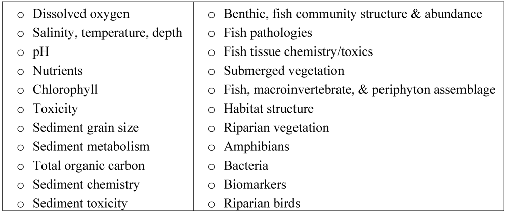
The technical, rather than intuitive, nature of most of these indicators presents a challenge to economic evaluation. Few of these “commodities” are in the realm of household or firm experience and the connection between them and commodities people perceive as important to their own welfare is unclear. (Boyd and Krupnick [61] discuss in more detail the ability to evaluate ecological measures generated by government analyses and programs through the lens of economics.)

Schiller et al. [62] conducted an analysis that presented EMAP indicators to focus groups of non-scientists. The focus groups were asked to evaluate the indicators, and found that the agency needed “to develop language that simultaneously fit within both scientists’ and nonscientists’ different frames of reference, such that resulting indicators were at once technically accurate and understandable”. While the study is not an economic analysis per se, it highlights the need for measures of ecological commodities that bridge the gap between natural science and goods and services to which economic value can be attached—a need being addressed by EPA’s Office of Research and Development [63,64].

We now briefly discuss the relationship between other common ecological indicators and their relationship to the ecosystem good and service indicators necessary to an ESI.

4.2.1. Biodiversity Measures

Consider biodiversity measures. Diversity indicators range from simple ones based on vegetation [65], to complex ones based on genetic diversity and polymorphism [66]. Economists have also contributed to the literature on biodiversity. In particular, Weitzman [67,68] has suggested a measure based on pairwise comparisons of the genetic distance between species or individuals. The measure also can be interpreted as the most likely taxonomic tree evolving from a common ancestor. Weitzman has extended this idea to policy rules for saving the greatest number of genes [69].

Biodiversity is a good example of how the interpretation of an ecological indicator as either an ecosystem service or an ecosystem asset can depend on context. If biodiversity has non-use value in itself, such measures may be a good measure of services. If biodiversity has value insofar as say, new pharmaceuticals are more likely to discovered if diversity is higher, diversity again may be considered a service input into pharmaceutical production, with a value equal to the marginal physical product multiplied by the value of drugs [70]. Finally, if biodiversity within a species is valued only insofar as it maximizes the likelihood of the survival of a species that is valued as a whole, it is not a measure of services at all. It may, however, still be a good measure of the future stream of services.

4.2.2. Biotic Integrity

The most commonly employed indicator system in government decision-making is the Index of Biotic Integrity (IBI). Many states and federal agencies use the IBI to assess aquatic resources, and the method has spawned a variety of derivative approaches geared toward terrestrial systems [71]. The system is composed of 12 indicators, six relating to the “composition and richness of species” and six relating to “ecological factors” [72]. The former include counts of particular species. The latter include measures of sampled fish health, including evidence of disease, damage, and anomalies. They also include so-called trophic factors, such as the prevalence of omnivores and top carnivores that help depict the flow of food and other energy through the system.

Biotic integrity measures are not well-suited to be service measures. Again, they are best thought of as indicators of asset quality. For the purpose of valuation, the trophic indicators are of scientific importance but are beyond the intuition of the public. Counts of individuals could be used as location-specific population indicators if they were related to species valued for recreation or their existence value, though the species counted in a typical IBI are neither. Similarly, a value potentially can be placed on deformity or disease in individuals, particularly if a connection to deformity in focal species can be made. The overall conclusion, however, is that the linkage between an IBI and outputs on which a value can be placed is weak. The point of an IBI, however, is to assess generally the quality of aquatic habitat. A good IBI score is not only good for the measured species but is presumed to be an indicator of the habitat’s ability to support a larger community of species interactions.

4.2.3. Hydrogeomorphic Assessment

Another index system is the hydrogeomorphic (HGM) approach developed to support regulatory decision-making regarding wetlands [73,74]. HGM has several characteristics worthy of note. Like the IBI, HGM makes a comparison between the study site and a reference site used to represent the baseline ecological condition (i.e., baseline asset quality). Second, position in the landscape is important. Third, it focuses on depicting site capacity to perform functions, including nutrient cycling, surface and groundwater storage, floodplain connectivity, organic carbon generation, retention of organic and inorganic particles, and provision of vertebrate habitat, plant communities, and aquatic food webs. Indicators thought to affect the performance of the eight basic functions are measured at each site. Like the IBI, the function measures generated by the HGM method are measures of asset quality, not flows of services.

4.2.4. Habitat Suitability

Another species-oriented index is the Fish and Wildlife Service’s Habitat Suitability Index (HSI). The indices are meant to characterize the carrying capacity of a habitat for one particular species. On a species-by-species basis, HSI relates habitat quality to observable biophysical characteristics derived from the scientific literature. For example, tree density or canopy cover may be related to a habitat’s species-specific carrying capacity. For aquatic species, indicators of things such as dissolved oxygen, salinity, water depth, substrate type, and toxicity would be combined in an HSI score.

HSI scores could be used as proxies for intangible or recreational benefits, but only for species that are perceived as important endpoints in themselves, such as endangered species. However, they are again measures of ecological asset quality not ecosystem service flows.

4.2.5. Other Ecological Indices

A range of other indices are worth noting in brief. The Environmental Protection Agency’s Environmental Indicators Initiative, for example, is designed to track biophysical conditions over time [75]. Indicators include air pollutant emissions, water quality measures, beach closings, and the prevalence of fish consumption advisories. The goal of the indicators is not economic measurement but scientific measurements that track environmental conditions over time.

The U.S. Department of Agriculture uses indicators in a variety of programs. The Forest Service, for example, reports a set of forest health indicators, including measures of crown condition, ozone injury, damage from disease, mortality, lichen communities, woody debris, vegetation diversity, and soil condition [76]. The Conservation Reserve Program has used an Environmental Benefits Index (EBI) to target enrollments in that program. The EBI uses a variety of indicators to derive scores for six endpoints: wildlife support, water quality, erosion, air quality, and conservation benefits. Example indicators include proximity to wetlands and conservation areas, soil erodibility measures, and distance-weighted population exposed to soil-related dust [77].

In addition to operational indicator systems, several national-level indices are worthy of note. A recent National Academies report recommended the generation of indicators related to species diversity: land cover and land use, nutrient runoff, soil organic matter, ecosystems’ capacity to capture energy, amount of energy and carbon that has been captured, carbon storage, stream oxygen levels; and the trophic status of lakes [78]. A heavily publicized report from the Heinz Center [79], used primarily to demonstrate significant gaps in data, called for the collection of numerous indicators relating to land use, aquatic resources, forests, agriculture, and other ecological conditions. Finally, a multi-agency report geared toward coastal issues recommended collection of seven basic water quality indicators: measures of clarity, dissolved oxygen, coastal wetland loss, benthic conditions, contamination of fish tissues, eutrophic condition, and sediment contamination [80].

Several conclusions should be drawn from this brief survey. First, while common elements do emerge, there is no scientific consensus or decision-oriented indicator system that should be the focus of a valuation-oriented ESI [54]. Second, ecosystem indices are not geared toward consumption-related endpoints. Ecological indices are thought of as a way to assess existing conditions, provide early warning of changes, and diagnose causes of environmental degradation [81]. In this respect—rather than as measures of service flows—they are suited to application in an ESI. Having said that, we also note that the growing adoption of an “ecosystem services perspective” in ecology is promoting the development of metrics designed to be more useful to economic assessment. For example, the literature on pollination services yields insights into the delivery of pollen to commercially valuable crops [82,83,84].

4.3. Predictive Bioeconomics: The Neuse Models

Economic analysis seeks tractable ecological production and damage functions to evaluate policy options and—in our case—to track economic welfare arising from ecosystem services. The importance of production functions, of course, is that they enable prediction of biophysical and economic outcomes. Unfortunately, ecology often does not yield easily quantifiable production functions with sufficient predictive power to be of direct use to economic assessment. In fact, contemporary ecology can be viewed as demonstrating that simple functional relationships do not exist—at least at a scale broad enough to be useful to economists [85,86]. Many functions are explored and depicted, but this tends to be the province of theoretical ecology rather than empirical ecology at a landscape level.

Increasingly, however, the problem of prediction is being addressed [87]. We consider in detail two innovative ecological production models, constructed by economists and ecologists, associated with a particular landscape context: the Neuse River watershed and estuary in North Carolina [20,21]. The models are of particular interest for two reasons. First, they address a predictive policy question, namely, the impact of reduced nutrient loadings on ecological outputs. Second, these predictions arise from a model in which a variety of ecological interactions take place.

In the language of this paper, the models feature asset–asset interactions and use these to predict ecosystem service flows. As we argued above, the linkage of sophisticated ecological analysis to economic outcomes is rare in ecology. (Just as sophisticated ecological modeling is rare in economics!) The Neuse models are ideally suited to an illustration of what we mean by depletion and depreciation adjustments. Because they are predictive—and innovative—the models can be used to show the challenges associated with the calculation of depletion and depreciation adjustments in an ESI.

They are also a way to convey the differences and similarities between an ecosystem services index and bioeconomic modeling. To do this, we will describe the models in the language of an ESI. Both papers explore the effect of reduced nitrogen loads on an estuarine-marine environment. They do this by tracing nitrogen load changes through a system of ecological interactions. In Smith and Crowder’s model [20], nitrogen loads affect algal stocks which, along with assumptions about sediment oxygen demand, allow the estimation of dissolved oxygen (DO) levels. DO then interacts with species and habitat variables—including growth rates, mortality, and the habitat’s carrying capacity—to produce estimates of crab and clam populations. The most ecologically distinctive element of the model is that these interactions are location-specific and location effects are linked via the migration of predators between patches.

Smith and Crowder construct a predictive model of spatially explicit, interacting ecological assets. Measurable indicators of these asset qualities include nitrogen concentrations, algal stocks, and DO. They also yield spatially distinct prediction of species abundance. Their model translates these, with the addition of harvest effort, into blue crab harvests. The ecosystem service may be defined as the value of blue crab stocks as a productive input to those harvests.

In Finnoff and Tschirhart’s model [21], a nitrogen load reduction leads to changes in algal populations of dinoflagellates and diatoms. Spatially explicit ecological interactions are also a feature of their model. The dinoflagellate and diatom populations are spatially distinct, being differentiated by water depth. These populations then interact with spatially distinct zooplankton, jellyfish, and clam communities. The populations of interest as outputs are two commercial species, croaker and blue crab. The spatially distinct populations are predicted, based on several predator–prey interactions, including between croakers and blue crabs themselves. As in Smith and Crowder [20], we are given a spatially explicit model with multiple ecological asset interactions that generates service flow estimates q. The model allows for services related to two spatially distinct blue crab populations, as in [20], and potentially croaker as well. Finnoff and Tschirhart [21] also raise the issue of accounting for croaker-related services even when these are exported outside of the geographic domain of the model. With the wider range of species included, one could imagine extending their model to clams and perhaps to (negative) non-use values for nuisance species like jellyfish as well.

How would we use the elements of the Neuse models in calculation of an ESI for the Neuse watershed? The ecological variable contributing to the production of crab harvests is simply the stock of crabs. Assuming this stock is measurable in principle via some sort of census, measuring the service raises no difficulties. A more challenging task is identifying the appropriate measure of the decline in the ecosystem assets arising from nitrogen deposition and depletion of the fishery and the adjustment of other species to those shocks, insofar as they affect future service flows.

To illustrate such a measure, we use model output from Finnoff and Tschirhart [21]. To first illustrate the construction of an index, we aggregate the crab services and croaker services. Although croaker is not included in the model, as the authors point out, this would be a natural extension. Our two measures of services s_i are thus blue crab and croaker populations, respectively. We construct an index of ecosystem services S^t for each of the 200 model-years by weighting each species population in year t by a constant price. These value weights are the marginal contribution of the stock, evaluated at the model parameters and at benchmark labor input (as measured by season length), multiplied by the wholesale price of blue crab and croaker, respectively [88]. Next, for the first 100 years of the model, we compute the present value of the next 200 years of ecosystem services, discounting at 3% [89]. Finally, we compute the change in this service flow, which is the depletion adjustment that we require.

The role of ecological indicators must be to compute this future flow of services. We test the ability of three common types of indicators to predict these changes in future services. The first indicator is the Simpson index of biodiversity, computed from the populations of all other creatures in the model. The second is a measure of water quality, specifically deep-water DO, which has been used in the HSI. In the model, DO can be proxied with the populations of dinoflagellates (algae). The third is the populations of species on which crab and croaker prey, namely deep-water zooplankton and clams. We also consider a combined model of DO and prey.

For each indicator, we regress the modeled change in the flow of future services on each of these indicators, for each case using three models consisting of 1-year lags in the indicators, 1- to 3-year lags, and 1- to 5-year lags. To illustrate the fit of these models, Table 1 reports the R² in each case as applied to the “business as usual” scenario and likewise Table 2 for the “30% nitrogen reduction” scenario.

Table 1. R² of Regression Using Various Lagged Indicators to Predict Changes in Future Ecosystem Services in a “Business as Usual” model of the Neuse River Estuary [21].

	Lags
Indicators	1	1 to 3	1 to 5
Simpson Diversity Index	0.00	0.13	0.15
Dinoflagellate population	0.00	0.58	0.64
Zooplankton and Clam Populations	0.70	0.88	0.92
Dinoflagellate, Zooplankton, and Clam Populations	0.72	0.93	0.96

Table 1. R² of Regression Using Various Lagged Indicators to Predict Changes in Future Ecosystem Services in a “Business as Usual” model of the Neuse River Estuary [21].

	Lags
Indicators	1	1 to 3	1 to 5
Simpson Diversity Index	0.00	0.13	0.15
Dinoflagellate population	0.00	0.58	0.64
Zooplankton and Clam Populations	0.70	0.88	0.92
Dinoflagellate, Zooplankton, and Clam Populations	0.72	0.93	0.96

Table 2. R² of Regression Using Various Lagged Indicators to Predict Changes in Future Ecosystem Services in a “30% Nitrogen Reduction” Model of the Neuse River Estuary [21].

	Lags
Indicators	1	1 to 3	1 to 5
Simpson Diversity Index	0.13	0.59	0.68
Dinoflagellate population	0.18	0.44	0.60
Zooplankton and Clam Populations	0.13	0.86	0.95
Dinoflagellate, Zooplankton, and Clam Populations	0.24	0.87	0.96

Table 2. R² of Regression Using Various Lagged Indicators to Predict Changes in Future Ecosystem Services in a “30% Nitrogen Reduction” Model of the Neuse River Estuary [21].

	Lags
Indicators	1	1 to 3	1 to 5
Simpson Diversity Index	0.13	0.59	0.68
Dinoflagellate population	0.18	0.44	0.60
Zooplankton and Clam Populations	0.13	0.86	0.95
Dinoflagellate, Zooplankton, and Clam Populations	0.24	0.87	0.96

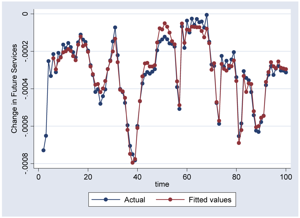
Not surprisingly, given that biodiversity per se plays no role in the Finnoff-Tschirhart model, the Simpson index generally does not predict future service flows well, especially in the business as usual scenario. DO, which directly affects fish respiration, performs somewhat better, with R² values of 0.64 and 0.60 using 5th order lags in the business as usual and 30% nitrogen reduction scenarios, respectively. However, in both scenarios the model using the population of blue crab and croaker prey—zooplankton and clams—performs best at each ordering of lags, with R² values as high as 0.92 and 0.95. Adding DO to these indicators improves the model further. Figure 2 illustrates the fit for the 5th-order model with zooplankton, clams, and DO.

A skeptic might suggest that we have merely recovered the model used to generate the results. However, we believe that the model illustrates that a small set of static, theoretically measurable indicators can capture the dynamic dependency of future service flows, even using a reduced form relationship in a context where “reality” (here, the Finnoff-Tschirhart model) is structural and more complex. Even the single indicator DO, the easiest to measure indicator of these examples, can explain 60% to 65% of the variation in changes in future service flows. Models using zooplankton and clams, probably the next easiest to measure if uniformly distributed spatially, provide an excellent fit.

Figure 2. Predicted vs. actual changes in future services using 5th order lags of zooplankton, clam, and dissolved oxygen indicators in a “business as usual” scenario.

Figure 2. Predicted vs. actual changes in future services using 5th order lags of zooplankton, clam, and dissolved oxygen indicators in a “business as usual” scenario.

Nevertheless, we also take this exercise as a cautionary tale of the difficulty associated with calibrated, equilibrium bioeconomic modeling. The time, resources, and expertise necessary to develop these models yield a fairly limited output from a public decision-making standpoint. Two limitations are worth noting. First, the full range of service impacts arising from a nitrogen load reduction will be much more expansive than impacts on the populations of two commercial species (a point the authors take pains to acknowledge). Second, the models did not need to confront the challenge of WTP estimation, since they were valuing ecosystem services with available market prices.

5. Indices of Willingness to Pay

In this section, we describe in more detail the dependence of benefits arising from services on the location, scale, quality, and timing of services. Benefits are the basis for the weights p_i assigned to particular services q_i in the ESI. In a consumption index of market goods, market prices are used as a proxy for WTP. If market prices for ecosystem services are absent, where are we to find reasonable proxies for WTP? One approach, which is highly arbitrary but appealing in its simplicity, is simply to use equal weights. In ecology, uniform weights are common (e.g., the IBI). One prominent non-ecological example is the United Nations’ Human Development Index [90], which weights equally three indicators of welfare: life expectancy, adult literacy, and GDP. Equal weighting can be defensible for two reasons. First, the choice of indicators employed in an index may exclude factors thought to have less weight than those included. Second, in the absence of more detailed, empirically demonstrable ecological relationships, equal weights are as good an assumption as any.

5.1. Willingness to Pay-Based Weights

However, our goal is a broad service index that captures an essential feature of ecosystem services; their quality and landscape location strongly influence the social benefits generated. WTP is inherently context-dependent. In particular, for those times and places where people value one service particularly highly, because of tastes, or a scarcity of that service, or scarcity of substitutes, the service in question would be given greater weight in the index.

Of course, WTP for ecosystem services raises several issues that are only marginally present in market-based accounts. Fundamentally, prices for ecosystem services are unobserved. Virtual prices would have to be estimated using non-market valuation methods [91]. Ideally, such methods would be applied to all the major services within the spatial scale of any particular ESI. Yet such an exercise would still raise a number of new implementation issues. For example, a spatial sample of virtual prices would have to be constructed differently than a sample of market prices as used in existing accounts. While market prices can be assumed to be largely constant within a single market, there is no arbitrage to ensure this condition for the implicit prices of environmental resources. Also, many ecosystem services are best thought of as differentiated goods with important place-based quality differences. As noted earlier, the biophysical characteristics of ecosystems are highly landscape-dependent [66,92,93,94,95]. The same is true of ecosystem services’ social benefits [96,97]. Accordingly, WTP for ecosystem services is best represented by a price function, not a single price.

As a general concern, we highlight one additional issue: The potential instability of preferences for ecosystem services over time in contrast to an index’s need for constant relative preferences across services [98]. Markets implicitly inform the development of preferences by facilitating exchange and educating consumers. Lacking the information provision and exchange properties of marketed goods, the average consumer of ecosystem services should not be expected to know as much about the factors that give rise to them or to their relative value. As a consequence, preferences for ecosystem services are likely to be less stable than preferences for conventional goods. This is a reason to pursue independent development of a value index (as described in Section 2) as a complement to a services index.

5.2. Building Weights via Benefits Transfer

When it is not feasible to conduct original non-market valuation for all the important services of an ESI in its specific spatial and temporal context, the transfer of virtual price information from other contexts is an alternative [99,100,101,102]. Ideally, to increase their applicability, benefits transfer analyses should adjust the estimates for differences in households and resources across contexts [103]. One approach to such adjustments is the structural meta analysis of Smith and Pattanayak [104] and Moeltner and Woodward [105]. Their approach calibrates the parameters of a preference function to benefits estimates in the literature, each viewed as a draw (with error) from different points on the function. This approach is particularly attractive when differences in incomes and other population differences are a priority. In the context of an ESI used in joint models of ecosystems and economic systems, it also would have the advantage of yielding index numbers for the ecosystem, consistent with the structure of preferences on the economic side of the model. However, this method may not be feasible when there are a large number of quality factors that affect WTP.

An alternative approach, which we introduce here, is a reduced-form regression of WTP on various factors. While this is an old approach for benefits transfer, econometrically speaking (e.g., [106]), our innovation is to introduce landscape-dependent indicators of the contribution of ecosystems to final goods and services and landscape-dependent indicators of substitutes and complements, as in Boyd and Wainger [107,108], as well as indicators of population differences.

WTP, while not directly observable, is a function of various characteristics that are observable. Let WTP weights p be denoted as a function G( ) of a vector of indicators I, so that

                                   p = G(I)                                    (9)

In principle, this function, on a service-by-service basis, can be calibrated by relating observable indicators I to existing WTP estimates of service value. If this were possible in practice, location and ecosystem-specific indicators I could be used to transfer monetary WTP estimates to locations where they are not available.

Currently, service-specific WTP estimates are too few in number to serve as a basis for such transfers across the national landscape. This particular empirical strategy is best thought of as an aspiration for an ESI. Nevertheless, we can lay out the basic strategy in more detail. We first derive a set of examples that connect the analysis of specific service flows to concrete data. The strategy in these examples is to first define a unit of account q_i. As discussed in section 3, the choice of units is driven largely by practical considerations.

With the unit of account defined, we identify a set of WTP proxies and organize them into three basic groups. First, because we are interested in social WTP, we look for population measures of the number of households or individuals likely to benefit from the service, to the extent that population is not captured in the service measure q_i. For example, the number of households within the viewshed of a natural area, the number of recreators with access to a stream or lake, the value of homes, businesses, and infrastructure protected from flooding by wetlands, or the number of homes being provided clean drinking water can be used to weight the service provided by a particular ecological feature (the service).

Second, we look for quality factors likely to affect WTP that are not captured in the definition of q_i. As discussed earlier, we might measure wetland-specific services. However, we may be able to rank the quality of particular wetlands by their proximity to sources of polluted runoff or likely flood pulses. These factors can be included to provide location-specific qualities that affect their weights p_i.

Third, we look for substitution and complementarity factors. Included in this category are measures of the scarcity of the service. Close substitutes for the service in question will depress willingness to pay for it, and thus the appropriate weight p_i. For example, the presence of abundant wetland resources in a region will tend to suppress any given wetland site’s value. Where visual amenities are concerned, WTP also will be related to the scarcity of the amenity within the viewshed. A measure of this is the availability of other acres of visible natural land cover, surface water, or other visually desirable land uses to residents of or visitors to the site’s viewshed.

For recreational services, like other applications, the importance of substitute recreation to WTP requires the definition of service areas or zones. In general, the relevant service area will differ depending on the service in question. A key methodological issue in any recreational benefits study is the determination of the appropriate “choice set” facing anglers, hunters, hikers, and birders. For a given recreational benefit, other forms of recreation are relevant as substitutes. We suggest substitution indicators at a variety of scales, local to regional. These indicators can then be empirically evaluated as part of the reduced form meta-analysis. For certain types of recreation, angling included, the relevant population may include transient vacation populations that can be assessed via tourism-related indicators.

WTP for ecosystem services will in some cases also be dependent upon the presence of complementary assets or services. This is particularly true in the case of recreational services, where access to natural areas is important. Access tends to be provided by complements, such as boat ramps, docks, and public parks and beaches.

WTP indicators—such as those presented above—can be used to leverage the results of relatively costly, time-consuming, and expert dollar-based WTP studies. Indicators, if properly validated, are the bridge between relatively isolated econometric studies and regional or national mappings of ecological benefits. The corollary, of course, is that the way we derive the weights p_i for use in an ESI is, by calibration, based on estimates arising from non-market valuation studies.

In general, note that the WTP indicators we propose can be thought of as the location-specific independent variables necessary to shift WTP estimates or functions in any benefit transfer study. Moreover, the landscape data that we argue is necessary to an ESI would be invaluable to any econometric analysis of environmental benefits.

We also note that weights can be derived in ways other than econometric analysis of revealed behavior. Expert elicitation, citizen juries, mediated modeling involving stakeholders, and even political referenda are all processes whereby weights are either explicitly or implicitly derived. Some of these methods may better respond to demands for collective learning and decision-making as an alternative or complement to more technical analysis [109]. In contrast to econometric estimation of weights, these alternatives involve a closer marriage of choices and learning. Typically, these methods involve a collective process whereby alternatives, relationships, and values are actively debated as part of the weighting process.

6. Conclusions

This paper draws upon ecological principles and the economic theory of index numbers to inform the design of an ESI. The design of an ESI first involves a sound theoretical underpinning—what we have termed the index’s architecture. The architecture highlights the factors necessary to a consistent treatment of preferences and ecological interactions and disciplines the choice of observable indicators relevant to the valuation of specific goods and services. For an ESI to be valid both economically and ecologically, a precise definition of ecosystem goods and services is required, in particular with a desire to avoid double-counting. Our definition, based on an analogy to GDP, makes use of a ready architecture to answer policy-relevant questions. It also clarifies the distinction between services per se and the value of services, and the concomitant need to use constant-value weights in the construction of an ESI.

An ESI generates ambitious implications for both the economic and ecological sciences. First, we identified the ways in which economics demands greater predictive power from theoretical and empirical ecology. This is no small challenge. Ecological prediction is extremely difficult, given the complexity of the biophysical phenomena in play and the lack of historical data amenable to predictive experiments. Moreover, compared to economics, prediction is less of a preoccupation within the biophysical sciences. In the near term, economists should try to accept (and treat sympathetically) the lack of predictive “production function”-based ecology.

The paper also proposes an econometric agenda for the validation of WTP estimates. This is a significant challenge in its own right. The challenge to this validation is not in the econometric methods necessary to the validation. Rather, the challenge is associated with the inherent difficulty of original dollar-based estimations and the conduct of a large enough number to validate the broad range of estimates an ESI requires.

In terms of the data required, much of it already exists. Importantly, many of the service measures and factors influencing WTP are available in a spatial format. As we have argued, this is particularly important because services, their quality, and their importance to welfare are strongly dependent on location. The federal government, states, counties, and localities currently collect geographic information systems data in accessible forms covering a large array of data types, including data on the presence of rare and endangered species, recreational opportunities, land cover, future land use, watershed land cover, floodplain characteristics, and roads and trails. Vast amounts of socioeconomic data, including population and other demographic data, are centrally distributed through the U.S. Census Bureau and are aggregated by census block, or block group, city, census tract, county, state, and for the nation as a whole. Federal and state databases, for example, cover census data by census tract, road networks, parks, housing and commercial and industrial buildings, public and private water supplies, historical sites, riparian and coastal characteristics, aquifers, and topography, among other things. Regional economic databases are available from several sources, such as the U.S. Department of Agriculture National Agricultural Statistics Service and the U.S. Bureau of Economic Analysis, for evaluating economic characteristics of regions of various sizes (counties, congressional districts, etc.) [107].

In the long run, an index of the ecosystem services enjoyed by society could play an important role in public policy. First, it could allow for a more comprehensive measure of well-being by acting as a non-market complement to existing national accounts. Second, an index of ecosystem services, many of them public goods, could provide the public with a marker of the ways in which government and private sector economic activity affect ecosystem-based well-being over time. As in the existing national accounts, an ESI would condense a set of complex information into a simple performance measure. Also, like the national accounts, this measure would prompt analysis, interpretation, and revision by a range of experts over time.

In the short run, an ESI might also be used in academic models of ecological and economic interactions. Such models must simplify reality by reducing the dimensionality of various services, and the theory of index numbers can provide a consistent way to do so. We have highlighted the most important factors required in making indexes consistent with preferences and with ecological interactions so that they might reflect the feedbacks between the two systems. Finally, insights from economic index numbers also can be used in models of pure ecology where reducing the dimensionality of the problem remains important.

Our architecture also helps illuminate the distinct roles of ecology and economics in measuring ecosystem services (including changes to future services) and values respectively. By the same token, it also highlights the points at which the two disciplines must come together to improve our understanding of the world we live in.

References

- Kneese, A.V.; Bower, B.T. Managing Water Quality; Resources for the Future: Washington, DC, USA, 1968. [Google Scholar]
- Boyd, J.; Banzhaf, H.S. What are ecosystem services? The need for standardized environmental accounting units. Ecol. Econ. 2007, 63, 616–626. [Google Scholar]
- Boyd, J. Nonmarket benefits of nature: What should be counted in green GDP? Ecol. Econ. 2007, 61, 716–723. [Google Scholar] [CrossRef]
- Fisher, B.; Turner, R.K.; Morling, P. Defining and classifying ecosystem services for decision making. Ecol. Econ. 2009, 68, 643–653. [Google Scholar]
- Fisher, B.; Kerry Turner, R. Ecosystem services: Classification for valuation. Biol. Conserv. 2008, 141, 1167–1169. [Google Scholar]
- The U.S. National Academy has repeatedly called for progress in this area [7,8]. Development of official green national accounts is currently moribund in the U.S.[9], though work continues by academics [10]. Internationally, however, a wide range of initiatives and pilot accounts are under development [11–15].
- Nordhaus, W.D.; Kokkelenberg, E.C. Nature’s Numbers: Expanding the National Economic Accounts to Include the Environment; National Academies Press: Washington, DC, USA, 1999. [Google Scholar]
- Beyond the Market: Designing Nonmarket Accounts in the United States; Abraham, K.G.; Mackie, C. (Eds.) National Academy Press: Washington, DC, USA, 2005.
- Boyd, J. Don’t Measure, Don’t Manage: GDP and the Missing Economy of Nature; Resources for the Future: Washington, DC, USA, 2008. [Google Scholar]
- Muller, N.Z.; Mendelsohn, R.; Nordhaus, W. Environmental accounting for pollution in the united states economy. Am. Econ. Rev. 2011, 101, 1649–1675. [Google Scholar]
- 11. Lange, G.M., Ed. Special issue on environmental accounting: Introducing the system of integrated environmental and economic accounting. Ecol. Econ.Year, 61, 589-723.
- Weber, J.-L. Land and Ecosystem Accounts in the SEEA Revision. In Position Paper for the UN London Group Meeting, Brussels, 2008.
- Schenau, S.; Delahaye, R.; Graveland, C.; van Rossum, M. The Dutch Environmental Accounts: Present Status and Future Developments; Statistics Netherlands: The Hague, The Netherlands, 2009. [Google Scholar]
- The World Bank, The Changing Wealth of Nations: Measuring Sustainable Development in the New Millennium; The World Bank: Washington, DC, USA, 2011.
- Green Accounting Virtual Resource Center. 2011. Available online: http://www.unep.ch/etb/areas/valuationEnvAcc.php (accessed on 20 March 2012).
- Wallace, K.J. Classification of ecosystem services: Problems and solutions. Biol. Conserv. 2007, 139, 235–246. [Google Scholar]
- Johnston, R.J.; Russell, M. An operational structure for clarity in ecosystem service values. Ecol. Econ. 2011, 70, 2243–2249. [Google Scholar]
- Peskin, H.M. A Proposed Environmental Accounts Framework. In Environmental Accounting for Sustainable Development; Ahmad, Y.J., Serafy, S.E., Lutz, E., Eds.; The World Bank: Washington, DC, USA, 1989; pp. 65–78. [Google Scholar]
- Hecht, J.E. National Environmental Accounting: Bridging the Gap between Ecology and Economy; Resources for the Future: Washington, DC, USA, 2005. [Google Scholar]
- Smith, M.D.; Crowder, L.B. Valuing ecosystem services with fishery rents: A lumped-parameter approach to hypoxia in the Neuse River Estuary. Sustainability 2011, 3, 2229–2267. [Google Scholar]
- Finnoff, D.; Tschirhart, J. Inserting ecological detail into economic analysis: agricultural nutrient loading of an estuary fishery. Sustainability 2011, 3, 1688–1722. [Google Scholar]
- Neary, J.P.; Roberts, K.W.S. The theory of household behaviour under rationing. Eur. Econ. Rev. 1980, 13, 25–42. [Google Scholar]
- Banzhaf, H.S. Green price indices. J. Environ. Econ. Manag. 2005, 49, 262–280. [Google Scholar]
- Based on marginal values, the ESI is a first-order approximation for consumer surplus (defined over multiple services). In his seminal text on index construction 80 years ago, Pigou [25] reasoned that the data necessary to compute WTP “are not, and are likely not, within any reasonable period of time, to become available to us…the only data which there is any serious hope of organizing on a scale adequate to yield a measure of dividend changes are the quantities and prices of various sorts of commodities” (p. 57).
- Pigou, A.C. The Economics of Welfare; Macmillan: New York, NY, USA, 1932. [Google Scholar]
- Färe, R.; Grosskopf, S.; Hernandez-Sancho, F. Environmental performance: An index number approach. Resource and Energy Econ. 2004, 26, 343–352. [Google Scholar]
- Fisher, I. The Making of Index Numbers: A Study of Their Varieties, Tests, and Reliability; Houghton Mifflin Co.: Boston, MA, USA, 1922. [Google Scholar]
- For full consistency, such a value index, paired with its symmetric service index, in general will not consistently factor the revenue index [27]. One of the two must be defined as an implicit index (i.e., as the revenue index divided by the other) or specific indices must be used, such as the Fisher index (the geometric mean of the Laspeyres and Paasche indices).
- This “fixed basket” interpretation of a price or marginal value index contrasts with the cost-of-living approach for “green price indices” suggested by [23]. That approach finds the cost of obtaining a fixed level of well being, allowing for substitution among ecosystem services, rather than the cost of a fixed basket.
- Costanza, R.; d’Arge, R.; de Groot, R.; Farber, S.; Grasso, M.; Hannon, B.; Limburg, K.; Naeem, S.; O’Neill, R.; Paruelo, J.; et al. The value of the world’s ecosystem services and natural capital. Nature 1997, 387, 253–260. [Google Scholar]
- Bockstael, N.E.; Freeman, A.M.; Kopp, R.; Portney, P.; Smith, V.K. On measuring economic values for nature. Environ. Sci. Technol. 2000, 34, 1384–1389. [Google Scholar]
- Weitzman, M.L. On the welfare significance of national product in a dynamic economy. Q. J. Econ. 1976, 90, 156–162. [Google Scholar]
- The necessity of being on this path is only one of several limitations to the result. See [7,34,35] for theoretical discussion.
- Weitzman, M.L. Income, Wealth, and the Maximum Principle; Harvard University Press: Cambridge, MA, USA, 2003. [Google Scholar]
- Dasgupta, P. The welfare economic theory of green national accounts. Environ. Resource Econ. 2009, 42, 3–38. [Google Scholar]
- Ehrlich, P.R.; Goulder, L.H. Is current consumption excessive? A general framework and some indications for the United States. Conserv. Biol. 2007, 21, 1145–1154. [Google Scholar]
- Heal, G.; Kriström, B. National Income and the Environment. In Handbook of Environmental Economics; Mäler, K.-G., Vincent, J., Eds.; Elsevier: Dordrecht, The Netherlands, 2005; pp. 1147–1217. [Google Scholar]
- Mäler, K.G. National accounts and environmental resources. Environ. Resource Econ. 1991, 1, 1–15. [Google Scholar]
- Mäler, K.G.; Aniyar, S.; Jansson, Å. Accounting for ecosystems. Environ. Resource Econ. 2009, 42, 39–51. [Google Scholar] [CrossRef]
- Repetto, R.; Rossini, F.; Beer, C.; Wells, M.; Magrath, W. Wasting Assets: Natural Resources in the National Income Accounts; World Resources Institute: Washington, DC, USA, 1992. [Google Scholar]
- U.S. Bureau of Economic Analysis. Integrated economic and environmental satellite accounts. Surv. Curr. Bus. 1994, 74, 33–49.
- Environment and Natural Resources Accounting Project (ENRAP). Report Prepared for the Philippine Department of Environment and Natural Resources; International Resources Group: Washington, DC, USA, 1996.
- Brock, W.A.; Xepapadeas, A. Valuing biodiversity from an economic perspective: A unified economic, ecological, and genetic approach. Am. Econ. Rev. 2003, 93, 1597–1614. [Google Scholar]
- O’neill, R.V.; Riitters, K.; Wickham, J.D.; Jones, B. Landscape pattern metrics and regional assessment. Ecosyst. Health 1999, 5, 225–233. [Google Scholar]
- Boyd, J. Location, Location, Location: The Geography of Ecosystem Services. In Resources; Resources for the Futrue: Washington, DC, USA, 2008; pp. 10–15. [Google Scholar]
- Olson, T. Biodiversity and Public Property: Conflict or Opportunity? In Biodiversity and the Law; Snape, W., Ed.; Island Press: Washington, DC, USA, 1996; pp. 67–79. [Google Scholar]
- Boyle, S.; Kanaroglou, P. Developing geographic information systems for land use impact assessment in flooding conditions. J. Water Resour. Plan. Manag. 1998, 124, 89. [Google Scholar]
- Kopp, R.J.; Smith, V.K. Valuing Natural Assets: The Economics of Natural Resource Damage Assessment; Resources for the Future: Washington, DC, USA, 1993. [Google Scholar]
- Suter, I.; Glenn, W. A critique of ecosystem health concepts and indexes. Environ. Toxicol. Chem. 1993, 12, 1533–1539. [Google Scholar]
- O’Neill, R.V. Is it time to bury the ecosystem concept? (With full military honors, of course!). Ecology 2001, 82, 3275–3284. [Google Scholar]
- National Research Council, Valuing Ecosystem Services: Toward Better Environmental Decision-Making; National Academies Press: Washington, DC, USA, 2004; p. 51.
- Shields, D.J.; Solar, S.; Martin, W. The role of values and objectives in communicating indicators of sustainability. Ecol. Indic. 2002, 2, 149–160. [Google Scholar]
- There are limits to how far we should push an ESI’s ability to capture such asset interactions. First, the biophysical sciences themselves have yet to characterize fully these relationships empirically. That is a process likely to take decades, if not longer. Further, many cause and effect relationships may be largely unquantifiable given the complexity of interactions among ecosystem components [30].
- Andreasen, J.K. Considerations for the development of a terrestrial index of ecological integrity. Ecol. Indic. 2001, 1, 21–35. [Google Scholar]
- Boyd, J. The Endpoint Problem. In Resources; Resources for the Future: Washington, DC, USA, 2007; pp. 26–28. [Google Scholar]
- Kontogianni, A.; Luck, G.W.; Skourtos, M. Valuing ecosystem services on the basis of service-providing units: A potential approach to address the ‘endpoint problem’and improve stated preference methods. Ecol. Econ. 2010, 69, 1479–1487. [Google Scholar]
- Hunsaker, C.T.; Carpenter, D.E. Ecological Indicators for the Environmental Monitoring and Assessment Program; Office of Research and Development, U.S. EPA: Research Triangle Park, NC, USA, 1990. [Google Scholar]
- Hunsaker, C.T. New concepts in environmental monitoring: The question of indicators. Sci. Total Environ. 1993, 134, 77–95. [Google Scholar]
- U.S. Environmental Protection Agency, Research Strategy: Environmental Monitoring and Assessment Program; Office of Research and Development, Environmental Protection Agency, National Health and Environmental Effects Research Laboratory: Research Triangle Park, NC, USA, 2002.
- U.S. Environmental Protection Agency, Generic Ecological Assessment Endpoints (GEAEs) for Ecological Risk Assessment; Risk Assessment Forum, U.S. Environmental Protection Agency: Washington, DC, USA, 2003.
- Boyd, J.; Krupnick, A. The Definition and Choice of Environmental Commodities for Nonmarket Valuation. In Discussion Paper; Resources for the Future: Washington, DC, USA, 2009. [Google Scholar]
- Schiller, A.; Hunsaker, C.; Kane, M.; Wolfe, A.; Dale, V.; Suter, G.; Russell, C.; Pion, G.; Jensen, N.; Konar, V. Communicating ecological indicators to decision makers and the public. Conserv. Ecol. 2001, 5, 19. [Google Scholar]
- Ringold, P.L.; Boyd, J.; Landers, D.; Weber, M. Report from the Workshop on Indicators of Final Ecosystem Services for Streams; U.S. Environmental Protection Agency: Corvallis, OR, USA, 2009. [Google Scholar]
- Ringold, P.; Nahlik, A.; Boyd, J.; Bernard, D. Report from the Workshop on Indicators of Final Ecosystem Goods and Services for Wetlands and Estuaries; U.S. Environmental Protection Agency: Corvallis, OR, USA, 2011. [Google Scholar]
- Defenders of Wildlife, Oregon’s Living Landscape: Strategies and Opportunities to Conserve Biodiversity; Oregon State University Press: Corvallis, OR, USA, 1998.
- Noss, R.F. Indicators for monitoring biodiversity: A hierarchical approach. Conserv. Biol. 1990, 4, 355–364. [Google Scholar]
- Weitzman, M.L. On diversity. Q. J. Econ. 1992, 107, 363. [Google Scholar]
- Weitzman, M.L. What to preserve? An application of diversity theory to crane conservation. Q. J. Econ. 1993, 108, 157. [Google Scholar]
- Weitzman, M.L. The Noah’s ark problem. Econometrica 1998, 1279–1298. [Google Scholar]
- Simpson, R.D.; Sedjo, R.A.; Reid, J.W. Valuing biodiversity for use in pharmaceutical research. J. Polit. Econ. 1996, 163–185. [Google Scholar]
- Canterbury, G.E.; Martin, T.; Petit, D.; Petit, L.; Bradford, D. Bird communities and habitat as ecological indicators of forest condition in regional monitoring. Conserv. Biol. 2000, 14, 544–558. [Google Scholar]
- Karr, J.R. Biological integrity: A long-neglected aspect of water resource management. Ecol. Appl. 1991, 1, 66–84. [Google Scholar]
- Brinson, M.M. A Hydrogeomorphic Classification for Wetlands. In Technical Report No. WRP-DE-4; U.S. Army Corps of Engineers Wetlands Restoration Program: Washington, DC, USA, 1993. [Google Scholar]
- Brinson, M.M.; Rheinhardt, R. The role of reference wetlands in functional assessment and mitigation. Ecol. Appl. 1996, 69–76. [Google Scholar]
- U.S. Environmental Protection Agency. Environmental Indicators Gateway. Available online: http://www.epa.gov/indicators/about.html (accessed on 21 January 2008).
- U.S. Fish and Wildlife Service, U.S. Fish and Wildlife Service Manual, 870 FW 1, Habitat Evaluation Procedures; U.S. Fish and Wildlife Service: Washington, DC, USA, 1996.
- Ribaudo, M.O.; Hoag, D.; Smith, M.; Heimlich, R. Environmental indices and the politics of the Conservation Reserve Program. Ecol. Indic. 2001, 1, 11–20. [Google Scholar]
- Ecological Indicators for the Nation; National Academy Press: Washington, DC, USA, 2000.
- The H. John Heinz III Center for Science Economics and the Environment. In The State of the Nation’s Ecosystems; Cambridge University Press: Cambridge, UK, 2002.
- U.S. Environmental Protection Agency, National Coastal Condition Report; Office of Research and Development and Office of Water: Washington, DC, USA, 2001.
- Dale, V.H.; Beyeler, S.C. Challenges in the development and use of ecological indicators. Ecol. Indic. 2001, 1, 3–10. [Google Scholar]
- Ricketts, T.H. Tropical forest fragments enhance pollinator activity in nearby coffee crops. Conserv. Biol. 2004, 18, 1262–1271. [Google Scholar]
- Kremen, C.; Ostfeld, R.S. A call to ecologists: Measuring, analyzing, and managing ecosystem services. Front. Ecol. Environ. 2005, 3, 540–548. [Google Scholar]
- Priess, J.; Mimler, M.; Klein, A.-M.; Schwarze, S.; Tscharntke, T.; Steffan-Dewenter, I. Linking deforestation scenarios to pollination services and economic returns in coffee agroforestry systems. Ecol. Appl. 2007, 17, 407–417. [Google Scholar]
- This may be in part because after initially borrowing from nineteenth century mechanical metaphors in a spirit similar to neoclassical economics, some ecology has turned to simulation methods that are not based on maximization or equilibrium concepts [85].
- Mirowski, P. Machine Dreams: Economics Becomes a Cyborg Science; Cambridge University Press: Cambridge, UK, 2002. [Google Scholar]
- Murtaugh, P.A. The statistical evaluation of ecological indicators. Ecol. Appl. 1996, 132–139. [Google Scholar]
- See equation 3.1 in [20]. The value of dB is 0.00178; the value of alpha-B is 0.75; the value of Beta-B is 0.25; and the benchmark value of T is 48. The wholesale prices of blue crab and croaker are $0.72 and $0.67, respectively.
- Finnoff and Tschirhart compute 200 years of model output. We assume the service flow for years 200 to 300 remain constant at year 200 levels.
- Anand, S.; Sen, A. Human Development Index: Methodology and measurement. In Human Development Report Occasional Papers (1992–2007); United Nations Development Programme: New York, NY, USA, 1994. [Google Scholar]
- Freeman, A.M., III. The Measurement of Environmental and Resource Values: Theory and Methods; Resources for the Future: Washington, DC, USA, 2003. [Google Scholar]
- Bockstael, N.; Irwin, E. Economics and the Land Use-Environment Link. In The International Yearbook of Environmental and Resource Economics 2000/2001; Tietenberg, T., Folmer, H., Eds.; Elgar: Cheltenham, UK, 2000; pp. 1–54. [Google Scholar]
- Gardner, R.H.; O’Neill, R.V.; Turner, M.G. Landscape-Scale Influences on Stream Habitats and Biota. In Humans as Components of Ecosystems: Subtle Human Effects and the Ecology of Populated Areas; Pickett, S.T.A., McDonnell, M.J., Eds.; Springer-Verlag: New York, NY, USA, 1993; pp. 208–226. [Google Scholar]
- Gustafson, E.J. Quantifying landscape spatial pattern: What is the state of the art? Ecosystems 1998, 1, 143–156. [Google Scholar] [CrossRef]
- Richards, C.; Johnson, L.B.; Host, G.E. Landscape-scale influences on stream habitats and biota. Can. J. Fish. Aquat. Sci. 1996, 53, 295–311. [Google Scholar]
- Heal, G.; Daily, G.; Ehrlich, P.; Salzman, J. Protecting natural capital through ecosystem service districts. Stanf. Environ. Law J. 2001, 20, 333–363. [Google Scholar]
- Bockstael, N.E. Modeling economics and ecology: The importance of a spatial perspective. Am. J. Agric. Econ. 1996, 78, 1168–1180. [Google Scholar]
- About this problem, Pigou [25] remarked that “the utmost we can hope for is a measure which will be independent of what the state of tastes and distribution actually is in either of the periods to be compared” (p. 58). For example, the Consumer Price Index is an adjustment used to value past output at current prices. In effect, GDP, when deflated this way, is recalculated for all past years and then compared to current-year GDP. Alternatively, GDP can value current output at past prices. The two calculations closely track each other but are not equivalent.
- Desvousges, W.H.; Johnson, F.R.; Banzhaf, H.S. Environmental Policy Analysis with Limited Information: Principles and Applications of the Transfer Method; Edward Elgar Publishing: Cheltenham, UK, 1998. [Google Scholar]
- Loomis, J.B.; Rosenberger, R.S. Reducing barriers in future benefit transfers: Needed improvements in primary study design and reporting. Ecol. Econ. 2006, 60, 343–350. [Google Scholar]
- Environmental Value Transfer: Issues and Methods; Navrud, S.; Ready, R. (Eds.) Springer: Dordrecht, The Netherlands, 2007.
- Rosenberger, R.S.; Loomis, J.B. Benefit Transfer. In A Primer on Non-Market Valuation; Champ, P.A., Boyle, K.J., Brown., T.C., Eds.; Kluwer: Dordrecht, The Netherlands, 2003. [Google Scholar]
- Loomis, J.B. The evolution of a more rigorous approach to benefit transfer: benefit function transfer. Water Resour. Res. 1992, 28, 701–705. [Google Scholar]
- Smith, V.K.; Pattanayak, S.K. Is meta-analysis a Noah’s ark for non-market valuation? Environ. Resource Econ. 2002, 22, 271–296. [Google Scholar] [CrossRef]
- Moeltner, K.; Woodward, R. Meta-functional benefit transfer for wetland valuation: Making the most of small samples. Environ. Resource Econ. 2009, 42, 89–108. [Google Scholar]
- Walsh, R.G.; Johnson, D.M.; McKean, J.R. Benefit transfer of outdoor recreation demand studies, 1968-1988. Water Resour. Res. 1992, 28, 707–713. [Google Scholar]
- Boyd, J.; Wainger, L. Landscape indicators of ecosystem service benefits. Am. J. Agric. Econ. 2002, 84, 1371–1378. [Google Scholar]
- Boyd, J.; Wainger, L. Measuring Ecosystem Service Benefits: The Use of Landscape Analysis to Evaluate Environmental Trades and Compensation. In Discussion Paper; Resources for the Future: Washington, DC, USA, 2003. [Google Scholar]
- Van den Belt, M. Mediated Modeling: A Systems Dynamics Approach to Environmental Consensus Building; Island Press: Washington, DC, USA, 2004. [Google Scholar]
© 2012 by the authors; licensee MDPI, Basel, Switzerland. This article is an open-access article distributed under the terms and conditions of the Creative Commons Attribution license (http://creativecommons.org/licenses/by/3.0/).
Share and Cite
MDPI and ACS Style
Banzhaf, H.S.; Boyd, J. The Architecture and Measurement of an Ecosystem Services Index. Sustainability 2012, 4, 430-461. https://doi.org/10.3390/su4040430
AMA Style
Banzhaf HS, Boyd J. The Architecture and Measurement of an Ecosystem Services Index. Sustainability. 2012; 4(4):430-461. https://doi.org/10.3390/su4040430
Chicago/Turabian StyleBanzhaf, H. Spencer, and James Boyd. 2012. "The Architecture and Measurement of an Ecosystem Services Index" Sustainability 4, no. 4: 430-461. https://doi.org/10.3390/su4040430