Downscaling of Short-Term Precipitation from Regional Climate Models for Sustainable Urban Planning

Abstract

A framework for downscaling precipitation from RCM projections to the high resolutions in time and space required in the urban hydrological climate change impact assessment is outlined and demonstrated. The basic approach is that of Delta Change, developed for both continuous and event-based applications. In both cases, Delta Change Factors (DCFs) are calculated which represent the expected future change of some key precipitation statistics. In the continuous case, short-term precipitation from climate projections are analysed in order to estimate DCFs associated with different percentiles in the frequency distribution of non-zero intensities. The DCFs may then be applied to an observed time series, producing a realisation of a future time series. The event-based case involves downscaling of Intensity-Duration-Frequency (IDF) curves based on extreme value analysis of annual maxima using the Gumbel distribution. The resulting DCFs are expressed as a function of duration and frequency (i.e., return period) and may be used to estimate future design storms. The applications are demonstrated in case studies focusing on the expected changes in short-term precipitation statistics until 2100 in the cities of Linz (Austria) and Wuppertal (Germany). The downscaling framework is implemented in the climate service developed within the EU-project SUDPLAN.

1. Introduction

Sustainable urban water management requires a storm sewer system that fulfils certain criteria, e.g., [1]. One is that the capacity should be sufficient to handle a low-frequency rainfall event, e.g., 10-year rainfall, without excessive flooding or other problems. Another is that—in case of combined sewer systems—the amount of sewer overflow should be as low as possible, in practice generally below some agreed limit. Sewer system design and evaluation is based on hydraulic simulations using short-term, local precipitation data as input. These simulations may be continuous, using long precipitation time series with many events as input, or event-based, using an observed or hypothetical single-event time series as input. In the latter case, the total storm volume is often obtained from Intensity-Duration-Frequency (IDF) curves that have been derived by extreme-value analyses of continuous time series, then a standardized design storm is used to estimate the temporal distribution, e.g., [2].

Climate change is expected to affect the precipitation process in different ways. A general trend towards more intense events has been suggested on theoretical grounds [3] and is generally supported by future climate model projections [4]. This implies that today’s sewer system design may not be sufficient to handle the future precipitation intensities [5]. To take the expected increase into account in the evaluation of a planned or existing sewer system requires an estimation of future precipitation data on the relevant temporal and spatial scales. This is difficult for various reasons. The resolution of available precipitation output from future projections made by Regional Climate Models (RCMs), are generally too low in both time and space. Thus some form of downscaling is required, which includes non-trivial statistical processing and programming. Further, even though RCM projection data may be available from web servers, downloading, interpreting and re-formatting the data takes a lot of resources in terms of both computer power and working time. This makes it very difficult, in practice virtually impossible, for a single urban planner or consultant to provide the input to urban hydrological climate change impact assessment studies.

To facilitate this type of local, urban climate change impact assessment, the EU-project SUDPLAN (Sustainable Urban Development Planner for Climate Change Adaptation; FP7-ICT-2009-6.4) was initiated. The aim is to develop an urban climate service, i.e., web-based tool through which the long term evolution of a range of hydro-meteorological variables (temperature, precipitation, runoff, air quality) can be incorporated in the urban planning process. In SUDPLAN the services will be requested from the Scenario Management System (SMS), which is a model control, visualization and integration workbench for the SUDPLAN Common Services (CS) as well as local models. CS offer downscaling services for rainfall, hydrology and air quality, provided that the user contributes with certain local data. Concerning short-term precipitation, the downscaling is based on the Delta Change method and is available for both continuous time series and single events/IDF curves. The short-term precipitation downscaling functionalities is being evaluated in two case studies; in Linz (Austria) where the focus is on combined sewer overflow and in Wuppertal (Germany) where the focus is on flooding. CS will contain an ensemble of RCM-downscaled GCM projections. In this description and demonstration of the downscaling methodology, results from two of the projections are shown in order to highlight both expected similarities and differences between projections when applied for this purpose. A complete climate change impact assessment requires the full ensemble to be used.

This paper starts with a background on downscaling of short-term precipitation from RCMs. This is followed by a description of the methodology developed and used in SUDPLAN and a demonstration of the performance in the Linz and Wuppertal case studies. Finally some conclusions are drawn and future prospects outlined.

2. Background

For urban hydrological applications and climate change impact assessments, precipitation data from climate models need to be downscaled as the scales of Regional Climate Models (RCMs) are larger than the scales of urban hydrological models. The latter typically work with a temporal resolution of a few minutes and a spatial resolution of a few km², i.e., the typical size of an urban catchment. In practice, precipitation data from one or a few local rain gauges are typically used. Concerning the temporal scale, the internal time step of RCMs is typically 15–30 min which is close to the urban scale. Often, however, output is not saved with this high resolution but maybe as 3-h or 6-h values. Concerning the spatial scale, the grid size of RCMs is typically 25 × 25 km (625 km²) or 50 × 50 km (2500 km²) which is far coarser than the urban scale. Precipitation intensities averaged over 1000–2000 km² are fundamentally different from point observations, with the former having a higher frequency of precipitation and lower extreme values. These differences increase with decreasing duration [6]. Therefore raw RCM precipitation data cannot be used in urban hydrological applications but needs to be downscaled.

There are different ways to perform (spatial) rainfall downscaling. One common way is to adjust the RCM rainfall based on local observations in a historical control period (bias correction) [7]. Another common way does not use the RCM rainfall but is based on statistical relationships between large-scale atmospheric circulation variables (e.g., pressure and wind) from the RCM and local rainfall [8,9]. A third way involves stochastic modeling of local rainfall with parameters estimated using RCM output [10]. A lot of work has verified the performance of these approaches on time scales of one day or longer, but for shorter time scales their applicability is limited. This is mainly because the statistical properties of local rainfall (extremes) strongly diverge from the properties of grid-scale rainfall when the time scale decreases. Also, the strength of relations between large-scale variables and local rainfall decreases for small time scales. Finally, the amount of sub-daily rainfall observations is far smaller than the amount of daily observations, which substantially increases the uncertainty in sub-daily adjustment and regression.

In SUDPLAN, another option—the Delta Change (DC) approach [11]—has been selected. In DC, no attempt to match RCM rainfall with observations is made. Instead the RCM rainfall is analyzed only with respect to future changes. Thus, some key property of rainfall (e.g., average annual rainfall) is calculated both for a long period representing today’s climate (often 1961–1990, traditionally) and an equally long period representing future climate (e.g., 2071–2100). The resulting relative change (e.g., 15% increase) is then transferred onto an observed time series, e.g., by multiplying all values by 1.15. By using this strategy, downscaling is achieved in the sense that the local nature of the observations is preserved, but with a modification that reflects some key aspect of the expected future change as given by the RCM.

DC was widely used in early hydrological climate change impact assessments and is still a main method, besides the ones mentioned above. Since the early applications, more elaborate ways to apply the procedure than only for average annual rainfall have been developed, e.g., by considering changes associated with different rainfall intensity levels [12,13]. In SUDPLAN, further development has been made (see Section 3 below).

It must be emphasized that DC has its limitations, the main one being the required assumption that changes in the rainfall properties calculated at the RCM grid scale are also valid for the local scale. This is not certain, as different rainfall mechanisms are dominant on different scales. Local rainfall extremes are generally produced by convective rainfall cells whereas grid-scale extremes may also be related to larger-scale, frontal-type rainfall systems. One aspect of this issue is that today’s RCMs are known to have a limited accuracy with respect to the description of local heavy rainfall [14]. Another aspect is that while the qualitative impact of global warming on high precipitation intensities is likely similar on all scales, the rate of change is not necessarily the same. Some studies suggest a future increase of rainfall intensity on the small/local scale than on the large/grid scale, based on both empirical data analyses [15] and climate model downscaling experiments [6]. This indicates that the grid-scale changes may be seen as a conservative estimate of the local changes. Another common limitation of DC is that a change in precipitation frequency, i.e., the fractions of wet (rainy) and dry periods, is generally not considered but the future frequency is assumed to be identical to today’s.

Despite the limitations, DC is conceivably the most robust approach to include in a general downscaling tool of the kind developed within SUDPLAN. Modification of local time series has the significant advantage that results (from e.g., an urban sewer model) obtained using the downscaled (i.e., Delta Changed) data may be directly compared with existing results from the historical data. As historical data are used in local models already, the downscaled data are directly applicable in the local models without another processing step. This is not the case in alternative downscaling approaches, which would also generate downscaled data for the historical period, i.e., simulated data that differ from the historical observations. Impact assessment would thus require an additional step of evaluating the ability of the RCM to reproduce today’s climate and the associated additional uncertainty.

3. Delta Change for Short-term RCM Precipitation Downscaling: Method Development

In SUDPLAN, the Delta Change approach is used for downscaling of both continuous observed short-term precipitation time series and event-based statistics (Intensity-Duration-Frequency (IDF) curves). In both cases, Delta Change Factors (DCFs) are calculated which represent the expected future change of some key precipitation statistic. In the downscaling, the estimated DCFs are applied to re-scale precipitation data representing today’s climate, generating realizations of local future short-term precipitation. The DCFs are estimated using RCM precipitation data from 30-year periods within which stationarity is assumed (non-stationarity may be implicitly explored using different 30-year periods).

3.1. Continuous Time Series

Time series downscaling is based on the version of the general Delta Change method described in [13]. Short-term precipitations from climate projections are analyzed in order to estimate future changes associated with different percentiles in the frequency distribution of non-zero intensities. The DCFs are calculated by dividing a certain percentile estimated in a future period by the same percentile estimated in a reference period; thus for time series DCF is a function of percentile. The DCFs may then be applied to an observed time series in the reference period, producing a realization of a time series in the future period. By applying this approach on a seasonal basis, it is possible to represent qualitatively different changes such as increase in peak intensities and decrease in total volume on different time scales, from entire seasons to individual events, which is required in light of expected future precipitation changes (see Section 4 below). In [13], a method to apply the DCFs to time series with a higher temporal resolution than the climate projection is outlined which is also used in the SUDPLAN tool. In the case of data from a tipping-bucket gauge, where the temporal resolution is further irregular, the DCF function is applied by considering the bucket volume as a variable.

As mentioned above, changes in precipitation frequency are generally not considered in DC applications. Distinct changes are, however, indicated in short-term precipitation from climate projections (see e.g., Section 4.2). From a hydrological perspective, this also implies changes insoil moisture dynamics which may impact, e.g., runoff generation and vegetation processes. As a result, frequency changes need to be considered in order to make accurate climate change impact assessments focusing on these and associated processes. In a study of daily precipitation projections for Belgium, one attempt at frequency adjustment was based on removing all precipitation from randomly selected (or isolated) wet days or adding precipitation to randomly selected dry days [16].

Within SUDPLAN an alternative approach has been developed. The approach is based upon the availability of short-term (sub-hourly) precipitation from climate projections which makes proper event-based analysis possible. In event-based analysis, precipitation events are extracted from a continuous time series and characterized in terms of, e.g., total volume, total duration and maximum intensity over different sub-durations. Also the dry periods between events may be extracted and their durations analyzed. A minimum dry period is required to separate between what should be considered independent events and what should be considered different parts of the same event. Different ways to estimate this minimum dry period have been suggested [17], but 2 h is a commonly used limit which is also used in SUDPLAN.

Future changes in precipitation frequency can be manifested in two different ways, or in a combination of these. One possibility is that the number of events remains the same but that their duration changes systematically towards longer or shorter. Alternatively, the durations remain the same but the number of events changes. Event-based analysis by the authors of 30-min precipitation from different climate projections in different regions indicate that the latter effect dominates, at least in a European perspective, i.e., frequency changes are related to changes in the number of events rather than their duration (see Section 4.2 below). This implies that for short-term precipitation, frequency adjustments should be performed on an event basis rather than random selection.

In the SUDPLAN frequency adjustment procedure, on a seasonal basis all events in the observed series are extracted and ranked with respect to “normality”, which is defined as the sum of the two absolute deviations (in %) of (1) the actual event volume from the mean event volume and (2) the actual event duration from the mean event duration. Also the dry periods are ranked similarly, where normality is naturally expressed only in terms of duration. In case of a projected decrease, the most normal events are removed, starting from the highest ranked and continuing until the proper frequency is reached (Figure 1a,b). In case of a projected increase in the precipitation frequency, the temporal precipitation distribution of the most normal events are copied and inserted to form new events in the most normal dry periods, starting from the highest ranked and continuing until the proper frequency is reached (Figures 1a,c). By involving the most normal precipitation events and dry periods in the procedure, unusual and extreme events remain untouched in the observed series which is considered desirable as they are more likely to affect subsequent impact assessment.

Figure 1. Schematic of the frequency adjustment procedure.

Figure 1. Schematic of the frequency adjustment procedure.

3.2. Extreme Events: IDF Curves and Design Storms

The downscaling of Intensity-Duration-Frequency (IDF) curves is based on extreme value analysis of time series of short-term precipitation data from climate projections. From the time series, annual maxima for a range of durations are calculated. The Generalized Extreme Value Type 1 (Gumbel) distribution is fitted to the maxima corresponding to each duration. The Gumbel distribution was selected based on analyses of short-term precipitation from an ensemble of climate projections over Sweden (unpublished) as well as sample locations in Europe. In these analyses, how well the Gumbel distribution fit to the annual maxima was similar to distributions with more parameters (see Section 4.3 below). The DCFs are calculated by dividing the Gumbel estimate for a certain combination of duration and frequency (i.e., return period T) in a future period by the same estimate in a reference period; thus for IDF curves DCF is a function of duration and return period. In order to reduce statistical scatter and obtain a robust relationship, multiple linear regression is used to express DCF as a linear combination of duration and return period, i.e.,

                    DCF = a₁ + a₂× D + a₃ × T                     (1)

where a₁–a₃ are regression coefficients.

The derived DCFs corresponding to a certain frequency may be used to re-scale a historical design storm. Two different approaches are conceivable. In the simplest case, all values of the design storm are re-scaled using the DCF corresponding to the total duration of the design storm. Alternatively, the dependence of DCF on durations shorter than the total duration is utilized. For example, a 1-h design storm could be re-scaled by first applying the 10-min DCF to re-scale the maximum 10-min period, then re-scale the maximum 20-min period to fit the 20-min DCF, and so on until the 1-h DCF is also matched, provided that the different DCFs are not conflicting but exhibit a consistent dependence on duration. However, as the DCF dependence on duration is generally weak for the durations generally considered when using design storms (up to 2–4 h; see Section 4.3 below), at least initially, the first, simpler alternative will be implemented in the SUDPLAN tool.

The design storm re-scaling functionality will allow for both static and dynamic applications. In the static case the catchment is considered homogeneous with respect to the rainfall intensity, i.e., rainfall movement is not taken into account but at a certain time step all parts of the catchment experience the same intensity. This is how design storms are typically used today, for small-scale urban applications. In this case the generation of future design storm will follow the simple approach outlined above. The second dynamic case represents a spatio-temporal extension of the design storm concept. In this case the catchment is considered heterogeneous with respect to the rainfall intensity, i.e., rainfall movement is taken into account and at a certain time step different parts of the catchment experience different intensities. Rainfall movement may have a significant impact on e.g., the discharge response in the sewer system [18] and should therefore be taken into account in a complete functional evaluation. The dynamic version is implemented by calculating the time lag in different parts of the catchment (based on given storm direction and speed) and then adjusting the static design storm appropriately [19]. It should be emphasized that the dynamic design storm functionality may be useful not only in a climate change context but also for evaluating the impact of movement in today’s climate, by generating dynamic versions of available static design storms.

4. Case Studies: Results and Discussion

The methodology outlined in Chapter 3 has been evaluated in two case studies within the SUDPLAN project; one in Linz (Austria) focusing on continuous time series and one in Wuppertal (Germany) focusing on extreme events. In both cases, short-term precipitation data are extracted from climate projections and analyzed with respect to key statistics and DCF relationships.

4.1. Climate Projections

Data from two GCM projections are used, one from the ECHAM5 model [20] and one from the HADCM3 model [21], both forced by IPCC emission scenario A1B [22]. Both GCM projections have been regionally downscaled to 50 × 50 km resolution over Europe by the RCA3 model [23]. In the following, the RCA3 projection based on ECHAM5 is denoted ECH and the one based on HADCM3 is denoted HAD.

For each of the case study locations, five RCA3 grid boxes were identified; the one covering the city and the one located in each quarter (i.e., N, S, E, W). From each grid box, two 30-year time series of 30-min precipitation was extracted; one reference period and one future period. Data from each grid box were analyzed separately, after which the results were averaged to get a representative result at the 50 km scale in the area under study. The reference period was selected to match the available observations and differed between the case studies (see Section 4.2), but the future period was in both cases 2070–2099.

4.2. Linz: Continuous Time Series

Linz is the capital of the Austrian federal state Upper Austria and is situated in the northern part of Austria directly at the Danube River. The city of Linz and its agglomeration have approximately 270,000 inhabitants. The Danube is the biggest Austrian river with a mean runoff of about 2000 m³/s at Linz. The average annual rainfall is 830 mm. For the urban drainage pilot in the SUDPLAN project, the whole of Linz and its 39 neighboring communes are of interest as they are drained together to one central wastewater treatment plant (WWTP) by a combined sewer system. In total this area covers approximately 900 km².

In combined sewer systems domestic and industrial sewage as well as storm water is transported together in the same pipe. In case of heavy rainfall, the combined sewage is in general either stored temporarily in the system or spilled out by combined sewer overflows in order to reduce the hydraulic pressure on the system and to limit the discharge to the WWTP. These overflows can have an important ecological impact on the receiving waters and are hygienically problematic. The sewer operator at Linz has put considerable effort and investments in storage facilities and control strategies in order to reduce the overflows and currently meets the Austrian requirements.

As rainfall is the most important driver of the runoff and overflow processes in a combined sewer system, information on possible future rainfall is crucial in order to develop proper mitigation strategies. This is also the major aim for the Linz Pilot in the SUDPLAN project: the SUDPLAN SMS will allow the operator to easily compare the effect of different future scenarios e.g., due to predicted rainfall by means of a simulation model. Details on the model are given in [24]. One local high resolution rainfall time series for Downtown Linz was available from the Austrian NIEDA tool [25]. Data is recorded by a tipping bucket rain gauge and is prepared especially for use in urban drainage modeling. Data are available fromthe period 1993–2006 and the 30-year reference period used in this case is 1981–2010.

In the observed time series, both monthly total precipitation and maximum 30-min intensity, here defined as the 99th percentile of the frequency distribution of non-zero values, is highest in summer (Table 1). In winter, the total precipitation is about half of that in summer and the maximum intensity 6–7 times lower. The characteristics for spring and autumn are rather similar, both being in between the values found for summer and winter. The wet fraction, a measure of occurrence defined as the percentage of 30-min periods with a non-zero precipitation, is consistently close to 10%, slightly lower in summer and slightly higher in winter.

The ECH projection indicates a pronounced relative increase (~25%) of the total autumn and winter precipitation, a smaller increase in spring (14%) and a clear decrease in summer (−14%) (Table 1). The annual cycle becomes flatter with all months approaching totals of 70–80 mm. The maximum intensity changes in all seasons, somewhat more in autumn and winter (~25–35%) than in spring and summer (~15–20%) but the shape of the annual cycle is largely preserved. The wet fraction shows a minor increase (~5–10%) in all seasons expect summer where it decreases by 16%. In summary, all considered aspects of precipitation (total, maximum, occurrence) increase in autumn, winter and spring. In summer only the maximum intensity increases; the total and the occurrence decreases. This illustrates the need for a flexible Delta Change approach that can manage e.g., contrasting trends for precipitation totals and maxima, respectively, as well as both positive and negative changes in the frequency of occurrence.

Table 1. Total precipitation (mm/month), maximum intensity (mm/30 min) and wet fraction (%) for all seasons in Linz in observations (OBS) and future projections ECH and HAD. For the projections, the percentage change is added in parentheses.

Season	Variable	OBS	ECH	HAD
Spring	Total	66.0	75.1 (+ 14)	72.4 (+ 10)
	Maximum	15.3	17.8 (+16)	17.3 (+ 13)
	Wet fraction	9.7	10.4 (+ 7)	10.3 (+ 6)
Summer	Total	99.2	85.3 (− 14)	95.3 (− 4)
	Maximum	26.8	32.2 (+ 20)	31.7 (+ 18)
	Wet fraction	8.9	7.5 (− 16)	8.4 (− 5)
Autumn	Total	58.3	71.2 (+ 22)	59.9 (+ 3)
	Maximum	9.4	12.8 (+ 36)	11.0 (+ 17)
	Wet fraction	8.6	8.9 (+ 4)	7.9 (− 8)
Winter	Total	55.2	69.8 (+ 26)	66.2 (+ 20)
	Maximum	4.2	5.3 (+ 27)	5.6 (+ 33)
	Wet fraction	10.9	11.8 (+ 9)	11.3 (+ 3)

Table 1. Total precipitation (mm/month), maximum intensity (mm/30 min) and wet fraction (%) for all seasons in Linz in observations (OBS) and future projections ECH and HAD. For the projections, the percentage change is added in parentheses.

Season	Variable	OBS	ECH	HAD
Spring	Total	66.0	75.1 (+ 14)	72.4 (+ 10)
	Maximum	15.3	17.8 (+16)	17.3 (+ 13)
	Wet fraction	9.7	10.4 (+ 7)	10.3 (+ 6)
Summer	Total	99.2	85.3 (− 14)	95.3 (− 4)
	Maximum	26.8	32.2 (+ 20)	31.7 (+ 18)
	Wet fraction	8.9	7.5 (− 16)	8.4 (− 5)
Autumn	Total	58.3	71.2 (+ 22)	59.9 (+ 3)
	Maximum	9.4	12.8 (+ 36)	11.0 (+ 17)
	Wet fraction	8.6	8.9 (+ 4)	7.9 (− 8)
Winter	Total	55.2	69.8 (+ 26)	66.2 (+ 20)
	Maximum	4.2	5.3 (+ 27)	5.6 (+ 33)
	Wet fraction	10.9	11.8 (+ 9)	11.3 (+ 3)

The future changes indicated in the HAD projection are similar overall to the changes in the ECH projection (Table 1). The sign of the change differs in only one case; the HAD projection indicates a slight decrease of the wet fraction in autumn, in contrast with the minor increase found in the ECH projection. Other notable differences concern the autumn total and maximum, which both increase much less in HAD than in ECH. Further, the decrease of summer total and occurrence are less pronounced in HAD than in ECH. In winter and spring all aspects change similarly in the two projections.

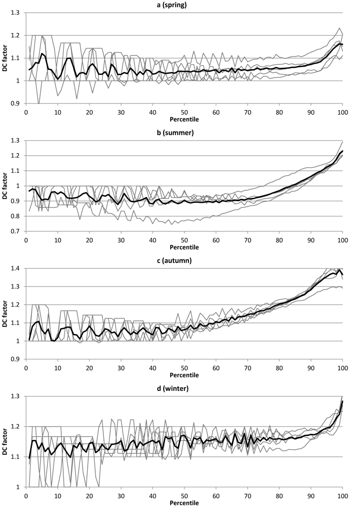
Concerning the DCF functions, these may be divided into two parts with different characteristics (Figure 2 and Figure 3). Below the 70th–80th percentile, the DCF functions fluctuate around a relatively constant average value that changes with the season. The average value is closely related to the change in precipitation totals (Table 1). In winter, with the maximum increase of total precipitation, the average DCF for low and intermediate percentiles is somewhere between 1.1 and 1.2. In summer, when total precipitation decreases in the projections, the average DCF is below 1. The constant DCF value approached for low and intermediate percentiles thus reflects the change found for the majority of intensities, which is manifested in the total precipitation. The notable fluctuations in the DCF functions, which are most pronounced for the lowest percentiles, are caused by the intensity resolution of the RCA3 precipitation data used here (0.01 mm/30 min). Low percentiles are close to this value, which creates sudden jumps in the DCF functions when the percentiles change with 0.01 up or down.

The spread between the different five grid boxes are dominated by the fluctuations related to the intensity resolution and therefore difficult to judge visually, but overall the spread around the mean DCF function (thick black line in Figure 2 and Figure 3) is limited and similar for all seasons.

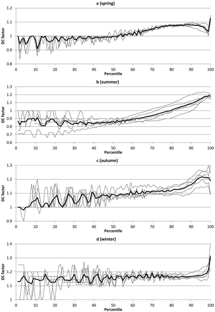
Above the 70th–80th percentile, the DCF functions are smoother and generally increasing towards their highest value at the 100th percentile. This implies that the highest future relative increase is expected for the highest short-term intensities. The general changes in maximum precipitation (Table 1) are reflected in the DCF value at the 100th percentile, being generally 1.3–1.4 in autumn and winter (Figure 2c,d and Figure 3c,d) and 1.1–1.2 in spring and summer (Figure 2a,b and Figure 3a,b). It should be emphasised that local precipitation extremes, relevant for, e.g., sewer system design, are generally generated by convective storms in summer. Thus the summer DCF values reflect the expected impact on design precipitation, even if these are lower than DCF values for other seasons. Some sudden bends are sometimes found in the DCF functions at the highest percentiles and these are caused by statistical variability of extreme intensities related to the most intense events. The smoothness of the functions reflects the fact that the intensity resolution has no impact on the DCF values for higher intensities. The spread between grid boxes for large percentiles varies from quite pronounced (e.g., Figure 3c) to very limited (e.g., Figure 3a) but overall the mean function is considered to represent the general patterns sufficiently well.

Comparing the two projections ECH (Figure 2) and HAD (Figure 3) indicates overall similar future changes of not only general aspects of precipitation (Table 1) but also in terms of the of the DCF functions. An obvious possibility is to parameterize the functions. This has been done in local applications of the approach, using simple expressions. However, it has turned out to be difficult to find a general parameterisation that is guaranteed to work satisfactorily for all attainable shapes of the DCF function and which generally, but not always, looks like the ones in Figure 2 and Figure 3. Further, careful weighing is required as the highest percentiles are generally the most important and must be well matched by the fit, but also the remaining part of the function must be satisfactorily reproduced. For these reasons, at least initially in the SUDPLAN tool, no parameterization is done but the empirical DCFs for each percentile are used in the re-scaling.

An event-based analysis of the two projections was made in order to evaluate the assumption behind the proposed approach to frequency adjustment (Section 3.1). A limit of 2 h was used to separate independent events and events with a total volume below 1 mm were not included. Four types of changes from the reference period to the future period were considered.

• ΔWF: relative change in the wet fraction, defined as above.
• ΔNE: relative change in the number of events.
• ΔEV: relative change in the average event volume.
• ΔED: relative change in the average event duration.

Figure 2. Delta Change (DC) factor as a function of percentile for all seasons in the ECH projection. Thin grey lines represent individual RCA3 grid boxes; thick black line is the average function.

Figure 2. Delta Change (DC) factor as a function of percentile for all seasons in the ECH projection. Thin grey lines represent individual RCA3 grid boxes; thick black line is the average function.

Figure 3. Delta Change (DC) factor as a function of percentile for all seasons in the HAD projection. Thin grey lines represent individual RCA3 grid boxes; thick black line is the average function.

Figure 3. Delta Change (DC) factor as a function of percentile for all seasons in the HAD projection. Thin grey lines represent individual RCA3 grid boxes; thick black line is the average function.

The changes of wet fraction ΔWF are overall similar to the ones reported in Table 1 but not identical as small events were discarded in the event analysis (Table 2). The main changes were a decrease in summer and an increase in winter. Concerning summer, in projection ECH the changes in average volume ΔEV and duration ΔED are very small but the projected decrease in wet fraction (−1%) is essentially only caused by a reduced number of events (−22%). The situation is less clear in projection HAD, which has notably fewer future events (−8%) but also a clear decrease of the mean duration (−12%). In both projections, the clear increase of the wet fraction in winter is mainly related to an increased number of events. In spring and autumn only smaller changes in the wet fraction are indicated, which are clearly related to changes in the number of events but also some changes in the event volume are indicated. In total, frequency adjustment by a changed number of events rather than changed event characteristics appears justified.

Table 2. Seasonal relative changes (%) in the wet fraction (ΔWF), number of events (ΔNE), average volume (ΔEV) and average duration (ΔED) between the reference and the future period in projections ECH and HAD.

Season	ΔWF		ΔNE		ΔEV		ΔED
	ECH	HAD	ECH	HAD	ECH	HAD	ECH	HAD
Spring	+9	+4	+10	+4	+3	+7	−2	+1
Summer	−21	−15	−22	−8	+3	0	−6	−12
Autumn	+8	−3	+7	−1	+21	+9	+2	−1
Winter	+22	+19	+23	+29	+11	+4	+2	−5

Table 2. Seasonal relative changes (%) in the wet fraction (ΔWF), number of events (ΔNE), average volume (ΔEV) and average duration (ΔED) between the reference and the future period in projections ECH and HAD.

Season	ΔWF		ΔNE		ΔEV		ΔED
	ECH	HAD	ECH	HAD	ECH	HAD	ECH	HAD
Spring	+9	+4	+10	+4	+3	+7	−2	+1
Summer	−21	−15	−22	−8	+3	0	−6	−12
Autumn	+8	−3	+7	−1	+21	+9	+2	−1
Winter	+22	+19	+23	+29	+11	+4	+2	−5

4.3. Wuppertal: Extreme Events

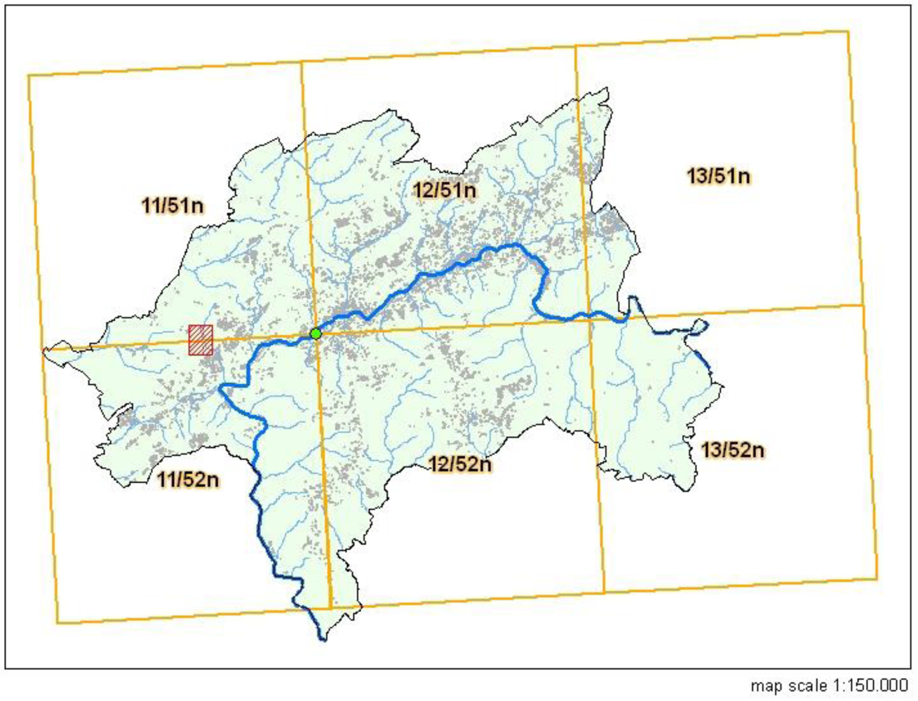
The city of Wuppertal, a town with approximately 350,000 residents, is situated in a hill country (~100–350 m.a.s.l.) in the state of North-Rhine-Westphalia in Germany. It is located in the valley of the river Wupper (Figure 4). There are several creeks on both sides of this valley that open into the storm water system before they finally end in the main receiving river Wupper. During heavy rainfall events the city’s storm water system is quickly blocked by those swollen creeks causing the precipitation to run off on the surface. The storm water runoff may thereby affect valuable public infrastructure and private property, as observed in the recent years in some of the creek catchment areas. Due to the complex geography it is completely unpredictable where a heavy rainfall event might occur and unknown whether there will be flooding.

Up to now the mid- and long-term planning of the storm water sewage system in Wuppertal has been accomplished with iterative model runs of a hydrological model (for the natural creeks) and a hydrodynamic model (for the canalized creeks and sewage system). Surface runoff was not taken into account in detailed simulations but by expert judgement. In the framework of the SUDPLAN-project the newly combined 1D-2D-hydrodynamical model DYNA-GeoCPM (www.tandler.com and Pecher Software) is used to detect critical spots with a high risk of flooding, e.g., regarding valuable and vulnerable facilities [26].

The aim is to mitigate the risk of flooding during serious storm events (return period T = 30 years or more) for the detected critical spots. The traditional strategies and measures to achieve this are either the enlargement of the storm water system profiles or the construction of retention basins. Given these two options the potential needs for investments would be immense, considering that the city faces inflow from 350 km of creeks and 650 km of storm water sewer systems. An alternative and much more cost-efficient strategy is to look for localized planning options which are likely to prevent damage. Examples of such structural measures are the alteration of street profiles by means of higher road curbs or the installation of mobile or stationary walls.

Figure 4. The city limit of Wuppertal with the test catchment Luentenbeck (red area) and the KOSTRA grid (yellow grid).

Figure 4. The city limit of Wuppertal with the test catchment Luentenbeck (red area) and the KOSTRA grid (yellow grid).

The SUDPLAN-platform will provide the responsible planners and hydraulic modelers in Wuppertal with a tool that enables them to simulate a multitude of scenarios with the model components for the sewer system and surface runoff, both to detect the critical spots and to simulate the effects of different structural measures at the critical spots. The tool should be able to store the parameters and results of such a model run and to visualize the results regarding climate change effects.

EULER II design storms for the Wuppertal pilot were calculated according to DWA-A 118 [2] based on the IDF curves described in [27]. The KOSTRA base data for calculating and regionalizing the precipitation amounts for duration periods between 24 h and 72 h consists of the daily 1 km gridded precipitation totals (1951–2000) using the REGNIE method (regionalization of precipitation totals in ~350,000 grid boxes). Short duration periods of the KOSTRA IDF curves are based on a collective of about 200 precipitation stations (1951–2000). The results from the actual analyses are being converted into the habitual KOSTRA 8.45 × 8.45 km grid with ~5350 grid boxes. It may be remarked that the area covered by the six grid boxes in Figure 4, ~430 km², corresponds to roughly 1/6 of an RCM grid box with the 50 × 50 km resolution used here. The test catchment area “Luentenbeck” for the Wuppertal pilot is located in the KOSTRA grid box 11/51 (Figure 4) and the corresponding 30-year intensities for a range of durations are given in Table 3. The reference period used in this case study is 1961–1990.

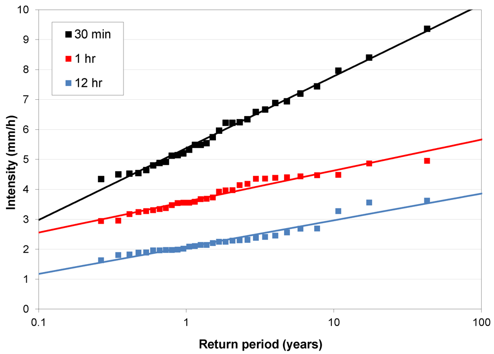
The Gumbel distribution fits to annual maxima for different durations calculated from time series from individual RCA3 grid boxes are generally very accurate (Figure 5). Some weak oscillations can be noted for the extracted maxima but in total the log-linear Gumbel fits are very good approximations.

Table 3. The 30-year precipitation depth (mm) in Wuppertal in KOSTRA data and future projections ECH and HAD. For the projections, the percentage change is added in parentheses.

Duration	KOSTRA	ECH	HAD
10 min	20.1	22.4 (+ 11) *	22.9 (+ 14) *
30 min	31.7	35.3 (+ 11)	36.1 (+ 14)
1 h	39.8	44.5 (+ 12)	45.4 (+ 14)
2 h	46.8	52.8 (+ 13)	53.6 (+ 15)
6 h	61.0	71.4 (+ 17)	71.2 (+ 17)
12 h	72.2	89.1 (+ 23)	86.5 (+ 20)

^* Extrapolated value.

Table 3. The 30-year precipitation depth (mm) in Wuppertal in KOSTRA data and future projections ECH and HAD. For the projections, the percentage change is added in parentheses.

Duration	KOSTRA	ECH	HAD
10 min	20.1	22.4 (+ 11) *	22.9 (+ 14) *
30 min	31.7	35.3 (+ 11)	36.1 (+ 14)
1 h	39.8	44.5 (+ 12)	45.4 (+ 14)
2 h	46.8	52.8 (+ 13)	53.6 (+ 15)
6 h	61.0	71.4 (+ 17)	71.2 (+ 17)
12 h	72.2	89.1 (+ 23)	86.5 (+ 20)

^* Extrapolated value.

Figure 5. Example of fitted Gumbel distributions (lines) to annual maxima (points) for different durations calculated from 30-min precipitation in one RCA3 grid box.

Figure 5. Example of fitted Gumbel distributions (lines) to annual maxima (points) for different durations calculated from 30-min precipitation in one RCA3 grid box.

Concerning the future change of the 30-year intensity in Wuppertal, the projection ECH indicates a clear dependence of the DCF function on the duration and towards larger changes for longer durations (Figure 6a). In fact, no change at all is projected for the shortest duration (30 min), or even a decrease (although this is conceivably caused by statistical variability in the extreme value analysis rather than reflecting a true signal), whereas an increase exceeding 30% (i.e., DCF > 1.3) is indicated for the longest durations considered (12–24 h). This type of duration dependence is in some contradiction with, e.g. a study of extreme short-term precipitation in Denmark from another RCM projection [4], in which an increase of DCF with decreasing duration is indicated. We can only speculate that the qualitative difference found is due to either a different response to global warming in the Wuppertal region or to differences in the descriptions of the precipitation process in the RCMs used. The spread between grid boxes is in the range 0.2–0.3 units; in particular one grid box stands out with consistently ~0.1 higher DCF than the average line. The projection HAD (Figure 6b) exhibits a principally similar dependence of the future change on duration, but the difference is smaller with DCFs ranging between 1.1 for 30 min to 1.25 for 24 h. The spread between grid boxes is smaller than for the ECH projection, being consistently in the range 0.1–0.2 units. In total, the spread is considered limited enough to meaningfully use the average change in subsequent downscaling. In the remaining part of this section, only changes averaged over all grid boxes are considered.

Figure 6. Delta Change (DC) factor as a function of duration for the 30-year intensity in Wuppertal in projection ECH (a) and HAD (b). Thin grey lines represent individual RCA3 grid boxes; the thick black line is the average function.

Figure 6. Delta Change (DC) factor as a function of duration for the 30-year intensity in Wuppertal in projection ECH (a) and HAD (b). Thin grey lines represent individual RCA3 grid boxes; the thick black line is the average function.

Concerning the dependence of the future change on frequency (i.e., return period), for projection ECH there is a tendency towards a larger increase for long durations as the return period increases (Figure 7a; point values). For the shortest duration the tendency is inversed towards a smaller future increase as the return period increases. For intermediate durations the dependence on return period is small, which makes the impact of return period small,also in the multiple linear regression used to obtain the final DCF functions (Figure 7a; lines). The DCF functions corresponding to return periods 1 and 10 years, respectively, are virtually identical whereas the 100-year function is located slightly higher. From visual inspection only, the fit of the final DCF functions to the individual curves may not seem impressive, but this is mainly due to the pronounced variability for durations of 30 min and 12 h. Overall, the magnitude and dependencies of the DCF values appear reasonably well captured. More advanced regression may be considered to obtain improved fits, but likely at the expense of a reduced robustness.

Figure 7. Delta Change (DC) factor as a function of duration for the T-year intensity in Wuppertal in projection ECH (a) and HAD (b). Point values represent original values; lines represent fits of Equation (1). The colors represent different return periods T = 1, 10 and 100 years.

Figure 7. Delta Change (DC) factor as a function of duration for the T-year intensity in Wuppertal in projection ECH (a) and HAD (b). Point values represent original values; lines represent fits of Equation (1). The colors represent different return periods T = 1, 10 and 100 years.

For projection HAD, the dependence on return period is less clear, although the same tendency as in the ECH projection is found for short durations (Figure 7b; point values). However, for the fitted DCF functions, contrary to the ECH projection, the 100-year function is located slightly below the other functions. Potentially, the dependence on the return period is unnecessary in the IDF curve downscaling, but this needs to be verified by further analyses. In the case of HAD, the fits are rather close to the individual curves for the entire range of durations. The weak dependence of DCF on the return period is in some contradiction with [4], in which a clear tendency towards higher DCF with longer return period was indicated for Denmark.

The future estimated changes of the 30-year intensities obtained from the fitted DCF functions are listed in Table 3. The value for a duration of 10 min has been extrapolated using the final functions. Overall, the two projections correspond well with respect to both the magnitude of change and the dependency on duration, as also seen in Figure 7. The 1-h values may be compared with the European analysis performed in [4], where an increase of ~20% was found for the same region between the same 30-year periods in another climate projection.

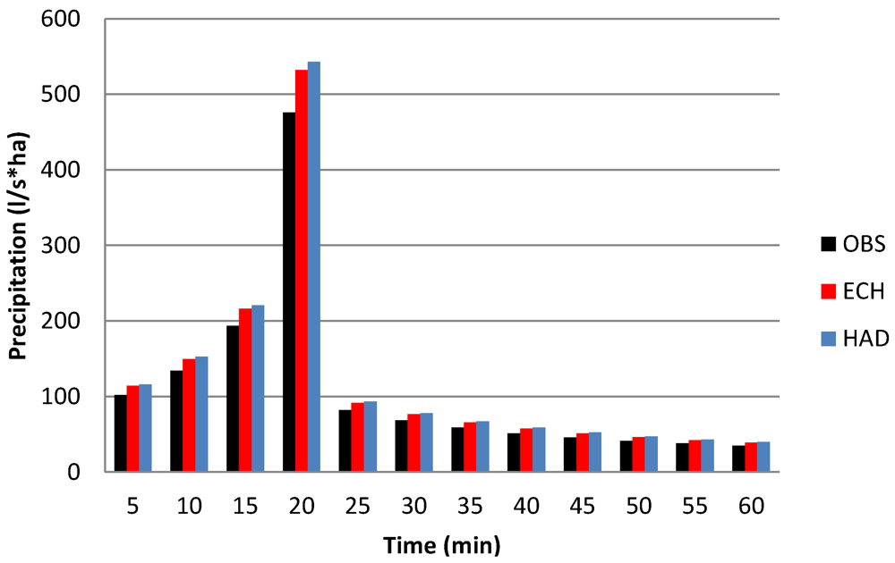
Finally, the 1-h EULER II design storm with a 30-year return period was rescaled in line with the projected future changes (Figure 8). All the individual 5-min values have been multiplied by the 1-hour 30-year DCF obtained from ECH (1.12) and HAD (1.14). As discussed in Section 3.2., in light of the weak duration dependence for short durations, this DCF value may also be assumed valid for shorter durations, down to the scale corresponding to the temporal resolution of the design storm (5 min).

Figure 8. Historical 30-year 1-h EULER II design storm for Wuppertal (OBS) and downscaled versions based on future projection ECH and HAD.

Figure 8. Historical 30-year 1-h EULER II design storm for Wuppertal (OBS) and downscaled versions based on future projection ECH and HAD.

5. Concluding Remarks

In this paper, a framework for downscaling precipitation from RCM projections to the high resolutions in time and space required in urban hydrological climate change impact assessment was outlined and demonstrated. The main challenge was to develop a robust and practical approach, suitable for Pan-European application in a wide range of precipitation regimes, based on state-of-the-art concepts. The basic approach is that of Delta Change (DC), developed for both continuous and event-based applications, which ensures that the downscaled data represent the precipitation process at the right temporal and spatial scales. Further, no difference exists between today’s climate as observed and as simulated, respectively. Alternative approaches would also generate simulated data for today’s climate that would differ more or less from observations and thus require an assessment of the uncertainty. This would take time, resources and competence that is not always available and the result is not necessarily more reliable. It should be emphasized that the developed procedures are deterministic. This is a limitation as there are certainly various sources of uncertainty involved in the DC applications, e.g., the variability between grid boxes. Providing probabilistically based output would be straight-forward, e.g., an ensemble of Monte-Carlo generated time series or IDF-curves with confidence intervals. Higher priority has, however, been given to providing output that the user may directly apply in impact studies with a minimum of additional work or processing, i.e., one data set in exactly the same format as the historical data. Uncertainty may be sampled by performing multiple downscaling simulations using different climate projections as input, a procedure strongly encouraged in the SUDPLAN tool.

As already mentioned, a required key assumption is that the future precipitation changes on the RCM scales used (30 min; 50 × 50 km) are representative also for smaller scales down to the ones relevant in urban hydrology (single minutes; single km²). The validity of this assumption is related to the different dominant precipitation mechanisms. It is known that current RCMs are mainly representing the properties of large-scale, frontal-type precipitation and fail to accurately reproduce the localized, convective, high-intensity events that dominate urban hydrological modeling and design [14]. This does, however, not necessarily mean that changes on the RCM grid scale are invalid for smaller scales. The question is whether the relative response to an increasing temperature is different for the different precipitation mechanisms and this issue is yet to be resolved. In general, the precipitation response at all scales is governed by the change in atmospheric moisture content with changing temperature. However, by theoretical considerations on processes limiting precipitation extremes, besides moisture content, also for example cloud dynamics on the small scale and available energy on the large scale, a somewhat higher increase (on the order of 5%) in small- than large-scale precipitation (extremes) with increasing temperature is conceivable, which is also supported in some empirical analyses and model experiments [15,28]. This implies that the changes in urban-scale precipitation (extremes) estimated using current RCMs is underestimated, but to a limited degree and that the RCM-estimated changes may be used as conservative estimates of the urban-scale changes. Currently, development of high-resolution (1–2 km²), convection-permitting RCMs is ongoing and the first future projections are about to become available [14]. These results are expected to shed substantially more light on this issue and provide credible estimates of the changes in urban-scale precipitation. However, such high-resolution RCM runs are extremely demanding in terms of computational power and it will take many years before ensembles of transient, continental-scale, high-resolution RCM projections are available.

Concerning future development of the DC approach, some possibilities exist. One is to provide probabilistic output, as described above. Another is to make the approach entirely event-based, by re-scaling events rather than individual values. This would possibly provide a more consistent procedure, but at the expense of increased complexity and not necessarily better results. To move from DC towards high-resolution RCM bias correction would require extensive, gridded and accurate high-resolution precipitation observations. Radar data have excellent resolutions in both time and space but consistent long-term sets are not yet commonly available and further careful quality control and adjustments are required to handle the various error sources involved. Concerning the SUDPLAN tool, extensive demonstration will take place in 2012 and the final product will become available by the end of the year. For more information, visit the SUDPLAN website [29].

References

1. Deutsches Institut für Normung (DIN), DIN-EN 752: Drain and Sewer Systems Outside Buildings; Beuth Verlag: Berlin, Germany, 2008.
2. German Association for Water, Wastewater and Waste (DWA), DWA STANDARD DWA-A 118E: Hydraulic Dimensioning and Verification of Drainage Systems; DWA: Hennef, Germany, 2006.
3. Trenberth, K.E.; Dai, A.; Rasmussen, R.M.; Parsons, D.B. The changing character of precipitation. Bull. Amer. Meteorol. Soc. 2003, 84, 1205–1217. [Google Scholar]
4. Larsen, A.N.; Gregersen, I.B.; Christensen, O.B.; Linde, J.J.; Mikkelsen, P.S. Potential future increase in extreme one-hour precipitation events over Europe due to climate change. Water Sci. Technol. 2009, 60, 2205–2216. [Google Scholar]
5. Hoppe, H. Impact of input data uncertainties on urban drainage models: Climate change a crucial issue? In Proceedings of the 11th ICUD International Conference on Urban Drainage, Edinburgh, UK, 2008.
6. Olsson, J.; Willén, U.; Kawamura, A. Downscaling extreme Regional Climate Model (RCM) precipitation for urban hydrological applications. Hydrol. Res. 2012, 43, 341–351. [Google Scholar]
7. Yang, W.; Andréasson, J.; Graham, L.P.; Olsson, J.; Rosberg, J.; Wetterhall, F. Distribution-based scaling to improve usability of regional climate model projections for hydrological climate change impact studies. Hydrol. Res. 2010, 41, 211–229. [Google Scholar]
8. Wilby, R.L.; Dawson, C.W.; Barrow, E.M. SDSM—A decision support tool for the assessment of regional climate change impacts. Environ. Modell. Softw. 2002, 17, 147–159. [Google Scholar]
9. Willems, P.; Vrac, M. Statistical precipitation downscaling for small-scale hydrological impact investigations of climate change. J. Hydrol. 2011, 402, 193–205. [Google Scholar]
10. Onof, C.; Arnbjerg-Nielsen, K. Quantification of anticipated future changes in high resolution design rainfall for urban areas. Atmos. Res. 2009, 92, 350–363. [Google Scholar]
11. Hay, L.E.; Wilby, R.L.; Leavesley, G.H. A comparison of delta change and downscaled GCM scenarios for three mountainous basins in the United States. J. Am. Water Resour. Assoc. 2000, 36, 397–397. [Google Scholar]
12. Semadeni-Davies, A.; Hernebring, C.; Svensson, G.; Gustafsson, L.-G. The impacts of climate change and urbanisation on drainage in Helsingborg, Sweden: Combined sewer system. J. Hydrol. 2008, 350, 100–113. [Google Scholar]
13. Olsson, J.; Berggren, K.; Olofsson, M.; Viklander, M. Applying climate model precipitation scenarios for urban hydrological assessment: A case study in Kalmar City, Sweden. Atmos. Res. 2009, 92, 364–375. [Google Scholar]
14. Kendon, E.; Roberts, N.; Senior, C.; Roberts, M. Realism of rainfall in a very high resolution regional climate model. J. Climate 2012. [Google Scholar] [CrossRef]
15. Lenderink, G.; Mok, H.Y.; Lee, T.C.; van Oldenborgh, G.J. Scaling and trends of hourly precipitation extremes in two different climate zones—Hong Kong and the Netherlands. Hydrol. Earth Syst. Sci. 2011, 8, 4701–4719. [Google Scholar] [CrossRef]
16. Ntegeka, V.; Baguis, P.; Boukhris, O.; Willems, P.; Roulin, E. Climate Change Impact on Hydrological Extremes along Rivers and Urban Drainage Systems. II. Study of Rainfall and ETo Climate Change Scenarios; Belgian Science Policy-SSD Research Programme; Technical Report for CCI-HYDR Project; K.U. Leuven-Hydraulics Section & Royal Meteorological Institute of Belgium: Leuven, Belgium, 2008. [Google Scholar]
17. Restrepo-Posada, P.J.; Eagleson, P.S. Identification of independent rainstorms. J. Hydrol. 1982, 55, 303–319. [Google Scholar]
18. Niemczynowicz, J. An Investigation of the Areal Properties of Rainfall and Its Influence on Runoff Generating Process; Report No. 1005; Department of Water Resources Engineering, Institute of Technology, University of Lund: Lund, Sweden, 1984. [Google Scholar]
19. Vaes, G.; Willems, P.; Berlamont, J. Moving design storms for combined sewer systems. In Proceedings of the 9th ICUD International Conference on Urban Drainage, Portland, OR, USA, 2002.
20. Roeckner, E.; Bäuml, G.; Bonaventura, L.; Brokopf, R.; Esch, M.; Giorgetta, M.; Hagemann, S.; Kirchner, I.; Kornblueh, L.; Manzini, E.; et al. The Atmospheric General Circulation Model ECHAM5. PART I: Model Description; MPI-Report 349; Max Planck Institute for Meteorology: Hamburg, Germany, 2003. [Google Scholar]
21. Gordon, C.; Cooper, C.; Senior, C.A.; Banks, H.; Gregory, J.M.; Johns, T.C.; Mitchell, J.F.B.; Wood, R.A. The simulation of SST, sea ice extents and ocean heat transports in a version of the Hadley Centre coupled model without flux adjustments. Clim. Dynam. 2000, 16, 147–168. [Google Scholar] [CrossRef]
22. Nakićenović, N.; Alcamo, J.; Davis, G.; de Vries, B.; Fenhann, J.; Gaffin, S.; Gregory, K.; Grübler, A. Special Report on Emissions Scenarios, Working Group III, Intergovernmental Panel on Climate Change (IPCC); Cambridge University Press: Cambridge, UK, 2000. [Google Scholar]
23. Kjellström, E.; Bärring, L.; Gollvik, S.; Hansson, U.; Jones, C.; Samuelsson, P.; Rummukainen, M.; Ullerstig, A.; Willén, U.; Wyser, K. A 140-year Simulation of European Climate with the New Version of the Rossby Centre Regional Atmospheric Climate Model (RCA3); Reports Meteorology and Climatology; Swedish Meteorological and Hydrological Institute (SMHI): Norrköping, Sweden, 2005; Volume 108. [Google Scholar]
24. Gamerith, V.; Olsson, J.; Camhy, D.; Hochedlinger, M.; Kutschera, P.; Schlobinski, S.; Gruber, G. Assessment of combined sewer overflows under climate change—urban drainage pilot study Linz. In Proceedings of IWA World Congress on Water, Climate and Energy, Dublin, Ireland, 2012.
25. hydro-IT, NIEDA—Die Niederschlagsdatenbank für Österreich—Manual Version 1.0.65; Hydro-IT GmbH: Innsbruck, Austria, 2007.
26. Sander, S.; Hoppe, H.; Schlobinski, S. Integrating climate change in the urban planning process—A case study. IFIP Adv. Inf. Commun. Technol. 2011, 359, 631–640. [Google Scholar]
27. Bartels, H.; Dietzer, B.; Malitz, G.; Albrecht, F.; Guttenberger, J. KOSTRA-DWD-2000 Starkniederschlagshöhen für Deutschland (1951–2000)—Fortschreibungsbericht; Deutscher Wetterdiens: Offenbach, Germany, 2005. [Google Scholar]
28. O’Gorman, P.A.; Schneider, T. Scaling of precipitation extremes over a wide range of climates simulated with an idealized GCM. J. Clim. 2009, 22, 5676–5685. [Google Scholar]
29. SUDPLAN homepage. Available online: http://sudplan.eu (accessed on 26 March 2012).