Exploring Future Impacts of Environmental Constraints on Human Development

Abstract

Environmental constraints have always had, and will always have, important consequences for human development. They have sometimes contributed to, or even caused, the reversal of such development. The possibility that such constraints, including climate change, will grow significantly this century raises the concern that the very significant advances in human development across most of the world in recent decades will slow or even reverse. We use the International Futures (IFs) integrated forecasting system to explore three scenarios: a Base Case scenario, an Environmental Challenge scenario, and an Environmental Disaster scenario. Our purpose is to consider the impact of different aspects and levels of environmental constraint on the course of future human development. Using the Human Development Index (HDI) and its separate components as our key measures of development, we find that environmental constraints could indeed greatly slow progress and even, in disastrous conditions, begin to reverse it. Least developed countries are most vulnerable in relative terms, while middle-income countries can suffer the greatest absolute impact of constraints, and more developed countries are most resilient. Education’s advance is the aspect of development tapped by the HDI that is most likely to continue even in the face of tightening environmental constraints, and that is one reason why human development shows great momentum even in the face of environmental challenges.

1. Introduction

Historians point to many occasions when environmental constraints contributed to, or caused, reversal of human development [1,2,3]. A number of such constraints will almost certainly intensify this century, jeopardizing the very significant advances in human development achieved across most of the world in recent decades.

We use the International Futures (IFs) integrated forecasting system to explore three scenarios with varying degrees of global environmental constraints. The IFs tool is well suited for this type of analysis because it models large-scale interaction of many relevant systems at global and country levels: demographic, economic, energy, agriculture, human capital (education and health), sociopolitical (domestic and international), physical capital (including infrastructure), environmental and technological. It is extensively data-based, rooted in theory, and widely used for long-term analysis. Section 2 describes the model in more detail.

The three scenarios explored in this paper are the Base Case (which includes some important environmental feedbacks and constraints), an Environmental Challenge scenario (which intensifies such constraints and broadens our attention to them), and an Environmental Disaster scenario (which explores the possible impact of truly vicious cycles and deterioration of systems in ways that may be extreme, but appear to be within the range of possibility). Each of these scenarios comprehensively considers impacts from a wide range of key global systems, not just environmental ones, and the latter two can be seen as environmental threat scenarios. Section 3 outlines the key assumptions underpinning the scenarios and explains their implementation in IFs.

The fourth section of this paper presents the results of our analysis. It uses the Human Development Index (HDI) and its separate components as our key measures of development (recognizing the many limitations of that measure, including its exclusion of sustainability considerations). We find that environmental constraints, considered broadly, could indeed greatly slow progress and even, with rather disastrous conditions, reverse it. Although such a reversal seems improbable to us, there is a great deal about the dynamics of environmental systems that scientists simply do not yet understand [4]. In the spirit of trying to better understand (1) the boundaries within which we had best maintain our relationship with the planet and (2) the potential for advancing human development, we explore the extent of slowing or reversal in HDI to which the Environmental Challenge scenario and the Environmental Disaster scenario might give rise.

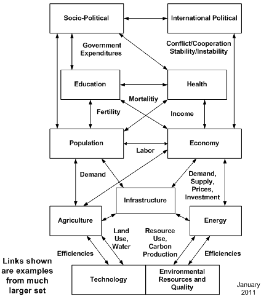
2. The International Futures (IFs) Model

International Futures (IFs) is a simulation model for analyzing country-specific, regional and global futures through alternative scenarios [5]. Although it is increasingly used in policy analysis, it began as an educational tool. Even in analysis applications, the primary strengths of the system are in framing investigation. Users of computer simulations should always treat forecasts as highly contingent scenarios, not as predictions.

IFs facilitates exploration of the long term future of closely interacting policy-related issues including human development (beyond the Millennium Development Goals), social change (including instability and risk), and environmental sustainability. It is a large-scale, long-term, fully integrated global modeling system (no sub-systems are exogenous to the others). It represents demographic, economic, energy, agricultural, socio-political, and environmental subsystems for 183 countries interacting in the global system (see Figure 1). The model is integrated with a large database for its many foundational historical series that largely begin in 1960 and earlier when available. The easy-to-use interface facilitates data analysis, forecast presentation, and scenario analysis.

Figure 1. The major modules of International Futures (IFs).

Figure 1. The major modules of International Futures (IFs).

IFs is a structure-based, agent-class driven, dynamic modeling system. The demographic module uses a standard cohort-component representation. The 6-sector economic module structure is general equilibrium seeking. The socio-political module represents life conditions, traces basic value/cultural information, and portrays various elements of formal and informal socio-political structures and processes.

The system facilitates scenario development and policy analysis via a scenario-tree that allows users to change framing assumptions, agent-class interventions, initial conditions or any relationship within the model. Scenarios can be saved for development and refinement over time. The easy-to-use interface also facilitates historical data analysis and display of forecasting results.

IFs is used increasingly widely. It was a core component of a project exploring the New Economy sponsored by the European Commission in 2001–2003 [6] and served the EC again in 2009 for a project examining the impact of information and communications technology (ICT) and on sustainability [7]. Forecasts from IFs supported the National Intelligence Council’s Project 2020: Mapping the Global Future [8] and Global Trends 2025: A Transformed World [9]. IFs provided driver forecasts for the fourth Global Environment Outlook of The United Nations Environment Program [10].

IFs is housed at the Josef Korbel School of International Studies at the University of Denver, and is available free of charge to download or use online [11]. Please access documentation on the website, through the model help system or via other IFs publications for more detail on the model structure and assumptions.

The population module:

• represents 22 age-sex cohorts to age 100+ in a standard cohort-component structure (but computationally spreads the 5-year cohorts initially to 1-year cohorts and calculates change in 1-year time steps)
• calculates change in cohort-specific fertility of households in response to income, income distribution, infant mortality (from the health model), education levels, and contraception use
• uses mortality calculations from the health model
• separately represents the evolution of HIV infection rates and deaths from AIDS
• computes average life expectancy at birth, literacy rate, and overall measures of human development (HDI)
• represents migration, which connects to flows of remittances.

The economic module:

• represents the economy in six sectors: agriculture, materials, energy, industry, services, and information/communications technology (ICT)
• computes and uses input-output matrices that change dynamically with development level
• is an equilibrium-seeking model that does not assume exact equilibrium will exist in any given year; rather it uses inventories as buffer stocks and to provide price signals so that the model chases equilibrium over time
• contains a Cobb-Douglas production function that (following insights of Solow and Romer) endogenously represents contributions to growth in multifactor productivity from human capital (education and health), social capital and governance, physical and natural capital (infrastructure and energy prices), and knowledge development and diffusion (research and development (R&D) and economic integration with the outside world)
• uses a Linear Expenditure System to represent changing consumption patterns
• utilizes a “pooled” rather than bilateral trade approach for international trade, aid and foreign direct investment
• has been imbedded in a social accounting matrix (SAM) that ties economic production and consumption to representation of intra-actor financial flows.

The agricultural module:

• represents production, consumption and trade of crops and meat; it also carries ocean fish catch and aquaculture in less detail
• maintains land use in crop, grazing, forest, urban, and “other” categories
• represents demand for food, for livestock feed, and for industrial use of agricultural products
• is a partial equilibrium model in which food stocks buffer imbalances between production and consumption and determine price changes
• overrides the agricultural sector in the economic module unless the user chooses otherwise

The energy module:

• portrays production of six energy types: oil, gas, coal, nuclear, hydroelectric, and other renewable energy forms
• represents consumption and trade of energy in the aggregate
• represents known reserves and ultimate resources of fossil fuels
• portrays changing capital costs of each energy type with technological change as well as with draw-downs of resources
• is a partial equilibrium model in which energy stocks buffer imbalances between production and consumption and determine price changes
• overrides the energy sector in the economic module unless the user chooses otherwise.

The environmental module:

• tracks annual emissions of carbon from fossil fuel use
• represents carbon sinks in oceans and forest land and models build-up of carbon in the atmosphere
• calculates global warming and links it to country-level changes in temperature and precipitation over time which, with the addition of carbon fertilization, impact agricultural yields
• represents indoor solid fuel use and its contribution to health related variables
• forecasts outdoor urban air pollution and links with respiratory disease
• models fresh water usage as a percentage of total water availability

The technology module:

• is distributed throughout the overall model
• allows changes in assumptions about rates of technological advance in agriculture, energy, and the broader economy
• is tied to the governmental spending model with respect to R&D spending

Other modules:

• education: forecasts rates of intake and completion across formal education levels for both sexes
• health: accounts for major causes of disability and death across major World Health Organization groups
• socio-political: represents government finance, social conditions, and attitudes of individuals, and qualitative and quantitative indicators of governance
• international political: traces changes in power balances and threat across states
• infrastructure: forecasts extent of and access to physical infrastructure categories

3. The Scenarios

For this analysis we used IFs to compare three scenarios: the Base Case scenario, an Environmental Challenge scenario and an Environmental Disaster scenario. This section explores the assumptions of these scenarios. The next section will evaluate the implication of the scenarios for human development indicators. All scenarios, as well as the model itself, are available on the Pardee Center for International Futures’ website.

3.1. The Base Case Scenario

A range of global transitions drive the Base Case forecasts of ongoing improvements in human development. Incomes continue to rise, driven in part by technological advances and diffusion globally. Education and health levels rise as incomes improve and reinforce economic growth. Advances in infrastructure and improved governance further drive productivity gains. Policy orientations and technological advances generally reflect those of recent decades. Table 1 outlines some important characteristics of the Base Case by issue area and variable. We expect, of course, many unforeseen changes to occur at all levels of analysis and across all systems, many of which will be the result of environmental problems; the Base Case is only a starting point for analysis.

Although the Base Case generally does demonstrate continuity with historical patterns, its complex dynamics, including a wide range of non-linear relationships, provide a structure that can also generate future patterns that are non-linear and differ from historical trajectories. Among such structural representations, the Base Case also includes important environmental constraints. For example, the use of solid fuels for cooking, outdoor air pollution and levels of access to safe water and sanitation all impact health. Also illustratively, temperature, precipitation and carbon fertilization [12] change agricultural productivity and affect food production and undernutrition (which in turn affects mortality in the short run and worker productivity through developmental stunting in the longer run).

The Base Case does not, however, consider large disruptive changes, be they natural, technological or policy-based. For example, the IFs model is not designed to identify sharp tipping points in natural systems such as dramatic shifts in the thermohaline circulation systems of our oceans or massive releases of greenhouse gas from melting of the permafrost, nor does it capture potential “overshoot” in all systems, especially environmental ones (although it does capture it in some, such as fossil fuel use). There is no representation of radical technology advances or their uses, such as the widespread uptake of carbon capture and sequestration or dramatic shifts in artificial intelligence. The Base Case does not build in carbon taxes or other significant shifts in global governance policy.

Table 1. International Futures Base Case Characteristics–Version 6.43.

Economy	Global GDP growth ranges from 3–3.5% annually	Economic production continues to diversify towards services and ICT	International trade as a percentage of GDP ticks up about 0.5 percentage points annually	Foreign Direct Investment as a percentage of GDP increases at nearly 0.04 percentage points annually	Foreign Aid more than doubles in 40 years from 6 trillion USD to over 12 trillion
Population	Fertility rates decline in all regions	Life Expectancy improves in all regions	Migration trends are extrapolated from historical patterns
Education	Primary education gross enrolment is over 100% by 2025	Secondary gross enrolment levels reach 80% by 2025	Tertiary gross enrolment is over 35% by 2040	World literacy levels are over 90% by 2030
Health	AIDS deaths fall to less than 1 million people annually by 2045	Communicable disease deaths decrease by half by 2040	Non-communicable disease deaths increase 1.5 times over 35 years	Global smoking rates decline to the level in 1980 in 25 years
Government	Political freedom increases at the global level	Economic freedom increases at the global level	Democracy improves	Corruption is reduced	Efficacy and Rule of Law are improved
Technology	Energy efficiency improves at 0.8% annually for first 15 years, then more quickly	Energy production costs decrease exogenously differently for each type covered (coal, oil, gas, hydro, nuclear and other-renewable)	Global convergence of productivity to system leader in technology
Agriculture	Cereal yields improve globally at about 0.03 tonnes per hectare per year	Overall crop land increases by about 1 million hectares per year	Overall grazing land increases by about 2 million hectares per year	Overall fish harvest remains constant
Energy	Energy from oil, gas and coal dominate global production for the next two decades	Renewable energy production surpasses any single fossil fuel by 2045	Hydro and nuclear energy production stagnate
Environment	Annual carbon emissions grow for the next 2–3 decades then decline	Carbon build-up in the atmosphere grows throughout the first half of the 21st century going beyond 500 PPM by 2050	Percent of population with no access to safe water below 10% by 2050	Global fresh water use reaches 10% of renewable by 2050, over 100% in North Africa by 2025	Indoor solid fuel use decreases below 20% of global population in 2050

Table 1. International Futures Base Case Characteristics–Version 6.43.

Economy	Global GDP growth ranges from 3–3.5% annually	Economic production continues to diversify towards services and ICT	International trade as a percentage of GDP ticks up about 0.5 percentage points annually	Foreign Direct Investment as a percentage of GDP increases at nearly 0.04 percentage points annually	Foreign Aid more than doubles in 40 years from 6 trillion USD to over 12 trillion
Population	Fertility rates decline in all regions	Life Expectancy improves in all regions	Migration trends are extrapolated from historical patterns
Education	Primary education gross enrolment is over 100% by 2025	Secondary gross enrolment levels reach 80% by 2025	Tertiary gross enrolment is over 35% by 2040	World literacy levels are over 90% by 2030
Health	AIDS deaths fall to less than 1 million people annually by 2045	Communicable disease deaths decrease by half by 2040	Non-communicable disease deaths increase 1.5 times over 35 years	Global smoking rates decline to the level in 1980 in 25 years
Government	Political freedom increases at the global level	Economic freedom increases at the global level	Democracy improves	Corruption is reduced	Efficacy and Rule of Law are improved
Technology	Energy efficiency improves at 0.8% annually for first 15 years, then more quickly	Energy production costs decrease exogenously differently for each type covered (coal, oil, gas, hydro, nuclear and other-renewable)	Global convergence of productivity to system leader in technology
Agriculture	Cereal yields improve globally at about 0.03 tonnes per hectare per year	Overall crop land increases by about 1 million hectares per year	Overall grazing land increases by about 2 million hectares per year	Overall fish harvest remains constant
Energy	Energy from oil, gas and coal dominate global production for the next two decades	Renewable energy production surpasses any single fossil fuel by 2045	Hydro and nuclear energy production stagnate
Environment	Annual carbon emissions grow for the next 2–3 decades then decline	Carbon build-up in the atmosphere grows throughout the first half of the 21st century going beyond 500 PPM by 2050	Percent of population with no access to safe water below 10% by 2050	Global fresh water use reaches 10% of renewable by 2050, over 100% in North Africa by 2025	Indoor solid fuel use decreases below 20% of global population in 2050

3.2. The Character of Global Environmental Challenges and Potential Disasters

It is extremely difficult to draw a clear boundary between environmentally-based and other challenges to human development. Considered most directly, environmentally-based challenges generally involve either constraints with respect to withdrawals of biophysical resources from global sources or constraints with respect to the use of global systems as sinks for outputs from human ones. Often, as in the case of dirtying our own drinking water, they involve both.

More broadly considered, however, there are many situations in which the consequences (often unacknowledged) of the uses of such sources and sinks, or of our efforts to avoid their use, pose major challenges to human development that have environmental bases that we do not automatically see as such. That is, there are many sometimes longer and more indirect pathways between environmental issues and human development. For example, something as seemingly removed from being an environmental issue as global aging has roots in environmental constraints. Malthus argued that preventative checks on population growth—such as increases in marriage age and the use of contraception—are unintentional adaptive measures of populations to limits posed by land and other resource limits. Humans can also be more intentional. Practices of households (e.g., primogeniture) or countries (e.g., the one-child family policy in China) flow from efforts to constrain population growth or its consequences in the face of limits. Aging populations, for better (e.g., demographic dividends) and worse (e.g., the dependent elderly), naturally follow from such demographic adaptations.

Similarly, in a world recognized as having plentiful capital and labor (and, in fact, having contemporary difficulties putting both to productive use), many of the forces restraining economic growth are, at the core, tied to environmental systems. For instance, one might attribute the so-called “lost decade of development” (the 1980s primarily) in many countries of Latin America, Africa and elsewhere to their having borrowed too much in global financial markets and become over-indebted. Yet cheap capital was a key driver of that borrowing, and it was fed by surpluses generated in oil-exporting countries when energy prices rose. Although the run-up in energy prices had triggers that were significantly political, the peaking of oil production in the United States and that country’s push into global energy markets in the 1970s contributed much foundationally, thus connecting growth constraints in the 1980s to environmental resource constraints in the 1970s.

In this section we step back and consider many of the challenges to economic growth and human development without being strictly bound by thoughts of immediate source and sink constraints. Then, in our scenarios, especially the Environmental Disaster scenario, we will draw upon broader sets of challenges in their framing.

One long-term global challenge that has an important environmental base—though not always explicitly identified as such—is the maintenance of a high rate of technological advance by leading countries as an engine of global economic growth. Whether one believes in the existence of fairly regular long-waves of such advance—often called Kondratieff cycles—there is no doubt that the pattern of economic growth varies significantly over relatively long periods of time. In the late 1960s global GDP growth sustained a 5-year moving average rate above 5 percent annually. That rate declined sharply in the 1970s, falling well below 4 percent and down to 2 percent in the 1980–1982 period. Through the 1980s and 1990s it mostly remained well below 3 percent, recovering to 4 percent only in the middle of the first decade of the new century (before being hit by a major global recession).

The lackluster performance of the 1980s (again, with fairly important roots both in energy and agriculture constraints) led Robert Solow to make his famous quip that, “You can see the computer age everywhere but in the productivity statistics” [13]. The pattern of economic growth in the U.S., the country generally defined throughout this period as the global technological leader, was not dramatically different, except for a surge of growth in the late 1990s—as would befit a country leading the information and communications technology (ICT) revolution. This surge preceded the rise of global economic growth over the next decade. Those who have worked to separate the impact of waves of technological advance from growth patterns affected by many other variables including energy prices (to be discussed below) generally associate shifts in economic growth from 0.2 percent to as much as 1.0 percent with historic advances such as steam engines (linked to the advantages of steam ships and railways, but also to shortages of wood in England before the coal age), electricity, and information and communications technology [14].

A related issue is whether other countries converge towards the technology, productivity and growth patterns of the technological leaders. The economic literature is colored with large debates about the extent of convergence and the reasons for its occurrence in some countries but not others. For instance, Sachs and Warner [15] argue that the key driver is adoption by poorer countries of generally efficient economic policies, significantly open trade, and protection of private property. When attention turns to environmental factors, those that receive attention are often geographic (such as being land-locked or resource poor [16,17]). Other studies, however, also look to environmental factors such as susceptibility to climate change [18].

The IFs Base Case builds in an assumption of constant patterns of technological advances for the system leader across the entire forecast horizon, variable by economic sector but contributing about 1 percent annually to productivity advances. The Base Case also represents a pattern of convergence by follower countries exhibiting an inverted-V character, so that middle-income countries are more able to adopt and benefit from leading-edge technology than the poorest. Around that pattern, advances in multifactor or total factor productivity depend on a wide range of physical, social, and human factors, many discussed below. Although some environmental factors (notably energy prices) affect that productivity, the model almost certainly under-represents such impact, suggesting the need to include additional environmental constraints exogenously in our scenarios.

Turning to energy issues, which clearly also contributed to the economic downturns of the 1970s and 1980s, M. King Hubbert produced one of the most famous and prescient forecasts when he predicted in the 1950s that U.S. oil production from the lower 48 states would peak between 1965 and 1970 (for foundational analysis see Hubbert 1949 [19]). Even with Alaskan production it peaked in 1970, contributing to rapidly rising global energy prices in the 1970s. The key uncertainty around global oil production is, of course, not whether it will peak but when [20]. Estimates generally range from now through 2040, depending not just on the rate of growth in production but also on assumptions about more unconventional sources such as tar sands and shale, as well as deep ocean drilling. Production in 54 of the largest 65 producers globally appears to have passed peaks, leaving large producers like Saudi Arabia in swing positions, and estimates of their future capacity are hotly debated [21].

The Base Case of IFs represents energy production not just of fossil fuels, but also of hydropower, nuclear power, and new renewable forms (in the aggregate) such as wind and direct solar energy. In the base case of IFs, global oil and gas production do not peak before 2030. That pattern is rooted heavily in the use by IFs of estimates on ultimately recoverable resources from the U.S. Geological Survey. The very rapid expansion in recent years, particularly in the United States, of natural gas production from shale formations through the use of hydraulic fracturing technologies greatly complicates understanding of resource bases, which the technology has undoubtedly expanded even as environmental debates rage around its use. The Environmental Challenge and Environmental Disaster scenarios consider more conservative assumptions than those of the Base Case.

In addition, the IFs Base Case makes assumptions about likely improvements in energy efficiency and reductions in costs of new renewable energy forms. These technological changes specific to energy (affected also by energy prices) are also difficult to forecast and could be overly optimistic [22]. If various constraints on energy in an Environmental Challenge scenario lead to higher energy prices, there will be an effect on economic productivity and growth; one generalized rule is that a rise in prices by $10 per barrel lowers growth in an economy like that of the U.S. by 0.2 percent [23].

Energy resources are, however, only one of the major global challenges posed by the interaction of humans with the environment via extraction from sources of needed inputs (e.g., energy, water, and forests) and dumping outputs (e.g., carbon, nitrogen, and phosphorus) into sinks. Rochström and others [4] identified nine “planetary boundaries” associated with such use of global biological and geological sources and sinks. They argued that we have already transgressed three of the boundaries, around climate change (associated with atmospheric levels of carbon dioxide and other greenhouse gases), rate of biodiversity loss, and the global nitrogen cycle (in their look at both the nitrogen and phosphorus cycles). The other boundaries they considered relate to ocean acidification, stratospheric ozone, freshwater use, land system change, chemical pollution, and atmospheric aerosol loading.

That study [4] also made clear the extent of uncertainty surrounding analyses of these boundaries and the impact of exceeding them [24]. Even with respect to one of the issues that has received most attention, namely atmospheric carbon levels, they pointed out the complications around their identified value of 350 parts per million (which is below current levels of about 390 ppm). For instance, they noted that contemporary climate models assess only “fast feedbacks” linking atmospheric carbon and global temperature, looking at those such as water vapor, clouds and sea ice. Fast feedbacks give rise to association of doubling pre-industrial CO₂ levels with a temperature rise of about 3 °C. Some analyses concerning inclusion of “slow feedbacks” such as decreased ice sheet volume, changed vegetation patterns, and flooding of continental shelves, suggest an impact of 6 °C. And, of course, this uncertainty about temperature change patterns precedes in impact analysis considerations of how atmospheric carbon might affect agricultural production. Because many variables affect yields, including the ability of scientists and farmers to adapt crops to new conditions, the uncertainty is considerable.

Even extensive analyses by Rochström and others [4] left potential challenges under-explored. For instance, with respect to water use, they focused on “green water” (soil moisture) and “blue water” (run-off). Among the major water issues facing many countries and regions, however, is draw-down of ground water faster than recharge (as in many parts of India and China) including heavy exploitation of extremely slow recharge fossil water in aquifers (as in Saudi Arabia and Libya), often with limited knowledge of the actual extent of such supplies.

The Base Case of IFs does forecast the build-up of atmospheric CO₂, the possible global temperature change associated with it, the associated country-specific changes in temperature and precipitation relative to 1990, and the impact of those changes on agricultural yields, even considering the positive or “fertilizing” impact that increased atmospheric carbon might have. It does not, however, represent the impacts of increased weather variability or of sea-level rise and coastal flooding. These are potentially very significant omissions. Also important, there is no direct constraint in IFs on future agricultural production from groundwater availability [25] (nor is there any explicit representation of possibly improved efficiency in the use of blue and fossil water).

Moving beyond biophysical challenges to social ones (and, as indicated earlier, these can stem from environmental forces), aging of populations is a major concern and pressure moving forward for many wealthy countries. In this area forecasts are relatively more certain than in energy systems. Yet the implications of these forecasts are relatively uncertain, in part because the health conditions of the elderly and possible political choices for care of them will become clearer only over coming decades. In democracies, of course, the elderly tend already to be a powerful political force and are unlikely to become more reticent in pursuit of their interests.

In addition to aging and for most developing countries a prior and more immediate challenge, the fertility transition to levels near or below replacement (about 2.1 children per average woman) is quite far from complete. In fact, in its 2010 Revision of data and analysis, the United Nations Population Division significantly revised upward its median population forecast (to 10.1 billion in 2100), arguing that the transition is proceeding more slowly than it foresaw earlier in many high-fertility countries, especially in Africa and Asia [26]. The Base Case forecast of IFs, with endogenous representations of changing fertility and mortality that we believe to be quite reasonable, produces numbers closer to the earlier 2008 Revision, including a peaking of global population well before 2100. Again, however, a more challenging scenario is possible.

Many other social factors will challenge humanity over the coming five decades. One of these is considerable and persistent conflict across ethnic and religious groupings—such groups are much less able to live in harmony when pressures of environmental constraints push peoples into competition for water, energy, and land. We may in fact be seeing an increasing trend in conflict between more fundamentalist groupings (with origins in all forms of religion) and more secular humans, as well as across the adherents to competing definitive truths. The Base Case of IFs does not explicitly build levels of domestic and international conflict on assumptions of increasing or decreasing religious, ideological tensions, or environmental constraints (on the link between the environment and conflict, see Homer-Dixon 1999 [27]; Raleigh and Urdal 2007 [28]; Busby, Smith, White and Strange 2010 [18]). The drivers often interact and the complexity of sorting them out suggests the importance of having alternative scenario assumptions.

Still other global challenges will almost certainly arise from international conflicts, again many times with deeper environmental foundations. The end of the Cold War ultimately resulted in both a reduction in direct intervention by great powers in the affairs of other countries (with especially notable exceptions such as the wars in Afghanistan, Iraq and Libya) and peace dividends for many governments in the form of lower defense spending as a portion of GDP. The rise of China, as well as of India and other large emerging states, will reshape the global high table in coming decades. Although accommodations to their rise, such as the creation of the G-20 grouping of countries to supplement the G-7, may head off many overt manifestations of conflict, the history of international politics in the face of challenges by rising states to system leaders is not a pretty one. Very often the sources of conflict between the declining hegemon and a rising power have been perceptions by the rising state of unfair division of access to a range of potential resources. Moreover, in the particular case of the rise of China, we are seeing an historically unusual transition from leadership by a high-income status-quo state to that of a middle-income emerging one (in fact, a set of them). That income gap near the top of the system has already helped frustrate a number of efforts to provide collective global public goods (such as the Doha round of trade negotiations and multiple high-level discussions on climate change). Even short of overt conflict over competing claims where multiple parties declare important national interests (such as the South China Sea and global financial balances), these difficulties could not just frustrate efforts around deepening important systemic connections such as open trade and financial flows, but even lead to some disruption of them (and of globalization more generally).

Not least among the global challenges will be the failure of the global community to raise the poorest, hungriest, and least-enabled human beings from abysmal conditions. In spite of much progress towards the Millennium Development Goals, there remain about 1.2 billion people living on less than $1.25 per day and in hunger. More than 300 million of these are in sub-Saharan Africa and while the IFs Base Case suggests that the still larger number in South Asia is likely to fall, it forecasts that there will still be more than 300 million in sub-Saharan Africa by 2060. Such numbers may prove to be overly optimistic as the IFs Base Case anticipates very substantial improvements in educational advances, extension of life expectancy (especially via reduction in the communicable disease burden), improvement in access to safe water and sanitation and reduction in the indoor use of solid fuels (a major killer).

Last, but not least, innumerable wild cards or fundamentally unpredictable negative events may dramatically shock human systems over the next half century. Taleb [29] referred to these as “black swans”: very low probability but high impact events. The fact that a few of them almost certainly will appear in the long-term future of nearly any complex system is one of the reasons for the optimism bias in the field of forecasting. Among those most often cited and perhaps of relatively higher probability is one with a mixture of environmental roots, namely plagues, related in part to density of populations and their close proximity in turn to animal populations [30]. Aging and therefore vulnerable populations, growing antibiotic resistance, the proven ability of pathogens to mutate, recombine, and also to jump across species all might seem to make a significant plague a low-to-medium rather than a very low probability event.

There are, of course, wild cards as well as underlying forces that could contribute very positively to global futures and alleviate many challenges. Those would include new and inexpensive energy sources or an African green revolution of major proportions. We will, however, continue to focus on the risks rather than the possibilities for luck and breakthroughs, turning next to the integration of challenges into Environmental Challenge and Environmental Disaster scenarios.

3.3. Environmental Challenge Scenario

Rooted in the considerations above concerning the extent of both missing linkages in the IFs system and uncertainties about the relationships between environmental variables and human development, the Environmental Challenge scenario changes the representation of the Base Case in two ways. First, it increases the driving values for a number of known environmental risks that the Base Case already represents, but that could prove to be worse than we anticipate. To do that we built on the foundation of an Environmental Risk scenario created earlier for work in forecasting global health (Hughes, Kuhn, Peterson, Rothman, and Solórzano (2011) [31], Hughes, Kuhn, Peterson, Rothman, Solórzano, Mathers and Dickson (2011) [32]). That work built on the modeling of the World Health Organization’s Global Burden of Disease project [33,34], (thanks in part to the generosity of Colin Mathers in making available the project’s formulations for forecasting mortality and morbidity by cause). The IFs project combined the distal driver health formulations of that project with proximate risk analysis building on WHO’s Comparative Risk Assessment project [35], which gave us the leverage points with which to create the Environmental Risk scenario. The scenario represents environmental risks at the household (indoor solid fuel use), local (water and sanitation), urban and regional (outdoor air pollution), and global levels (especially increasing impacts of global warming on agricultural production). In each case it moves the patterns for countries approximately one standard error in a less optimistic direction from a cross-sectionally estimated function linking GDP per capita at PPP (as a rough proxy for development level) and levels of risk in countries around the world.

To represent additional environmental challenges not necessarily captured by the IFs system or represented in the relatively narrow focus of the Environmental Risk scenario, we further expanded the Environmental Challenge scenario by drawing also on insights from the United Nations Environment Programme Global Environmental Outlook 4 scenario exercise [10]. For the GEO 4 project the IFs system built scenario representations of four different scenarios (Policy First, Markets First Sustainability First, and Security First) [36].

Of those four, the Security First scenario represents a number of the broader challenges to global futures emanating from environmental forces, many of which are secondary spill-over effects. The types of impacts captured in Security First include a retreat from openness and globalization. In this scenario, states increase protectionism from trade, decrease democracy, lower levels of domestic economic freedom, increase inequality and reduce flows of foreign direct investment. (Although increased autonomy and associated slower economic growth could potentially increase environmental security in the long term, this scenario was framed by the perspective of domestic focus on the pursuit of shorter-term economic and physical security.) This series of interventions increases the probability of state fragility. These choices lower levels of economic growth relative to the base case and impact human development across a range of systems.

The resultant Environmental Challenge scenario, pulling together most aspects of the foundational Environmental Risks and Security First scenarios, represents a considerably darker world than the IFs Base Case (see Box 1 for the basic elements). We shall look at the impacts on human development later in the paper.

Box 1. The Environmental Challenge Scenario.

The Environmental Challenge scenario

All changes are relative to underlying dynamic values. For instance, an increase in fertility would be relative to underlying rates that are decreasing for almost all developing countries. The scenario introduces almost all changes over a period of years, because large, sustained changes seldom happen instantaneously.

Technology/productivity. Reduces the overall rate of systemic technological advance by 0.5 percent and slows the rate of convergence by other countries to the leader. Both China and India, as rapidly emerging countries with high growth rates, lose 2.0 percent annual convergence; South Central Asia and Africa, as especially vulnerable regions, lose 1.0 percent annual convergence; the rest of the world loses 0.5 percent.

Energy. Lowers the rate of progress in cost reduction for production of renewable energy by 50 percent.

Agriculture. Positing impacts on yield from environmental factors not in the model, the scenario slows growth in agricultural yield by 0.5 percent annually to a total of 25 percent. Posits a growth of undernutrition in part related to distribution of 1 percent annually relative to the decline of the base case to 50 percent above the Base Case. Reduces global supplies of fresh water by 25 percent over 50 years (0.5 percent annually). Turns off the effect of carbon dioxide on crop fertilization.

Demographic. Increases fertility rates of non-OECD countries by 10 percent over 60 years. Slows down the global reduction of fertility by 0.15 percentage points over 10 years.

Socio-political. Global and domestic changes occur in interaction. Reduces global migration by 25 percent over 10 years. Increases protectionism on trade by 20 percent over 5 years. Reduces flows of foreign direct investment by 40 percent over 5 years. Reduces economic freedom by 10 percent over 15 years. Reduces political democracy (and the freedom measure) by 10 percent over 15 years. Increases military spending by 20 percent over 10 years. Increases domestic inequality by 15 percent over 20 years.

Millennium Development Goal progress. With respect to health-related MDGs, the scenario slows down progress towards improved and household-connected water and sanitation by 50 percent over 50 years and increases urban air pollution and indoor use of solid fuels by the same amount.

Health. Focusing only on HIV/AIDS directly, increases the death rate globally from AIDS by 20 percent over 20 years, slows down the peaking of HIV prevalence in sub-Saharan Africa by 8 years, and increases the peak incidence in sub-Saharan Africa by 4 percentage points.

Conflict. Increases the probability of intrastate conflict by 20 percent over 20 years.

3.4. Environmental Disaster Scenario

Environmental Disaster is the third scenario compared in this set (see Hughes, Irfan, Moyer, Rothman, and Solórzano (2011) [37] for an elaborated presentation). We have emphasized that there are great uncertainties surrounding current and future environmental challenges (direct or via complex pathways) and the human response to them. Overuse of fossil water and falling water tables, changing run-off patterns from glacial melting, progressive deforestation and land degradation, species loss and dramatic declines in biodiversity, accelerated incidence of extreme weather events, peaking production of oil and gas (which this analysis has largely ignored except for conservative analysis of it in the Base Case), and much more will greatly stress bio-physical and human systems in coming decades. The full potential for associated vicious feedback loops is unknown.

To address these uncertainties in any precise manner is, of course, impossible. They remain uncertainties. Therefore this scenario manipulates fundamentally the same interventions as the Environmental Challenge scenario, but amplifies their magnitude in most cases. For instance, the overall reductions in systemic economic advance, and that in specific countries and regions are roughly doubled relative to Environmental Challenge. Similarly, the increase of fertility rates is roughly doubled, and the reduction in agricultural yield is about twice as fast. With respect to factors around globalization, the protectionism in trade is approximately twice as great; migration declines by about 75 percent instead of 25 percent. In addition to increased military spending, we reduce public education spending significantly in the scenario. The use here of characterizations such as “roughly”, “about”, and “approximately” is deliberate, because the model is a dynamic system and equilibrating mechanisms often partially offset interventions of this kind (although frequently at a cost, such as increased agricultural investment to partially offset decreased yields).

Although we view this as a very low probability scenario, at least in the time horizon of our forecasts, the individual assumptions are all possible. Moreover, it is by no means a worst case scenario. There exist possibilities, for instance, of either physical or social systems reaching tipping points that fundamentally change equilibrating patterns.

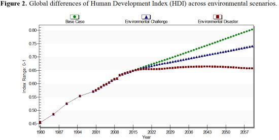
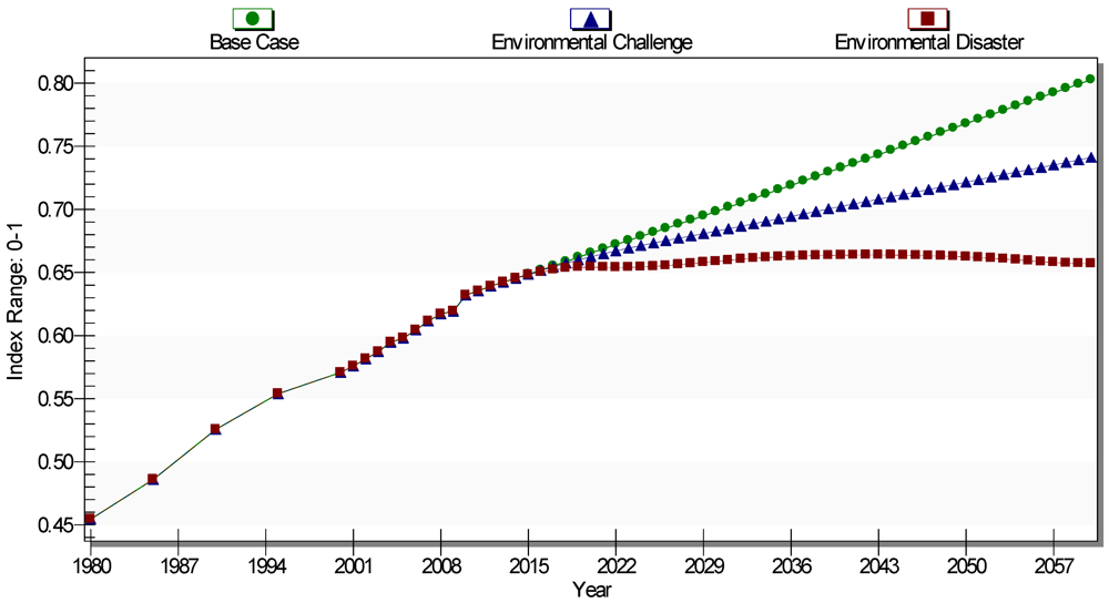
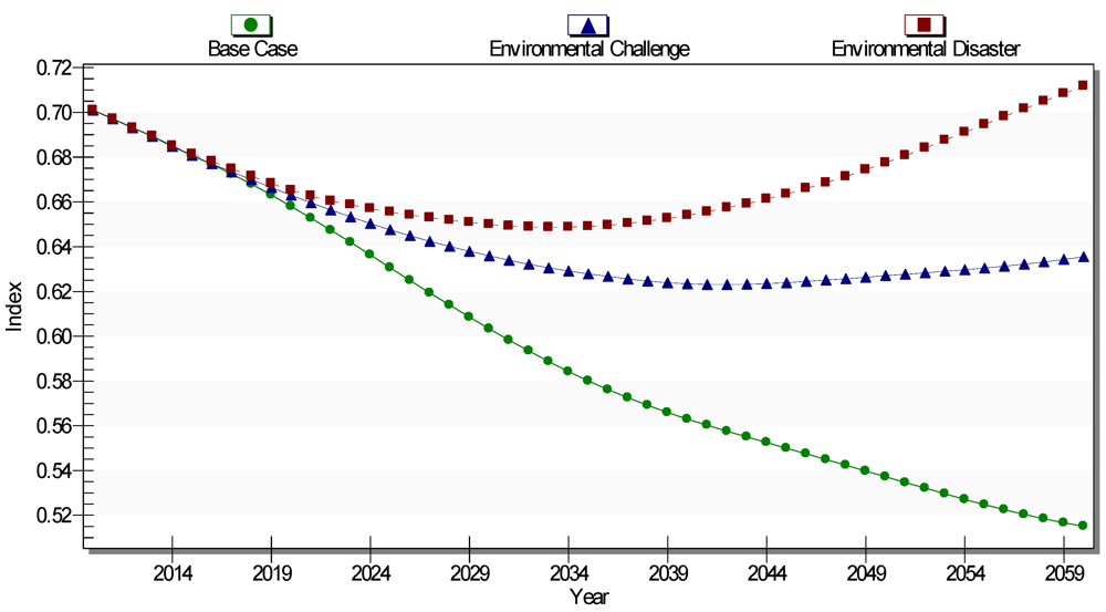
4. Scenario Impacts on Human Development

To see the results of the environmental constraints we will look ahead 50 years to 2060. This is the time horizon of the Pardee IFs Center’s series on Patterns of Potential Human Progress (see Hughes, Irfan, Khan, Kumar, Rothman, and Solórzano (2008) [38] on reducing global poverty; Dickson, Hughes, and Irfan (2009) [39] on advancing global education; and Hughes, Kuhn, Peterson, Rothman, and Solórzano (2011) [31] on improving global health). We begin by comparing the scenarios globally with respect to values of the Human Development Index (reformulated in 2010; UN Human Development Program (2010) [40]). Then we will turn to the various dimensions of the index: health, knowledge or education, and income. In each case we will consider also patterns for countries at different income levels or in different regions. We also devote attention to the equity implications of the alternative scenarios.

4.1. Environmental Impacts on Human Development: The HDI

In IFs we compute both the original Human Development Index (HDI) and that reformulated in 2010 as a long and healthy life (indicated by life expectancy), knowledge (as measured by mean years of schooling for adults age 25 and older and expected years of schooling), and a decent standard of living (as measured by the log of GDP [41] per capita at PPP). Figure 2 shows the HDI historically since 1960 and in the IFs forecasts for the three scenarios [42]. In the Base Case global HDI reaches 0.803 in 2060. Although the pattern of growth through that year appears nearly linear, the forecast is not an extrapolation, but rather the dynamic result of the interactions of all model components across 183 countries (aggregated to the global total with population weighting). Even in the Base Case, HDI growth is slower than it has been historically. Although that is in part a result of the environmental constraints in the scenario, it is also in part a result of the built-in saturation effects of the index’s construction. Not only does the logarithmic term on GNI per capita contribute mechanically to such saturation, so more substantively do the inevitable slowing of increments in years of formal education in the middle- and high-income countries, the likely slowing of advance in life expectancy of cutting-edge countries like Japan, and the even more certain decline in speed of convergence by low- and middle-income countries as the health and education gaps with high-income countries narrow. In contrast to the 2060 global value of 0.803 in the Base Case, the HDI reaches only 0.741 in the Environmental Challenge scenario and only 0.657 in the Environmental Disaster scenario (almost unchanged from the value of 0.632 in 2010).

Figure 2. Global differences of Human Development Index (HDI) across environmental scenarios.

Figure 2. Global differences of Human Development Index (HDI) across environmental scenarios.

The impact of environmental constraints on different sets of countries varies, of course. Figure 3 shows the global difference between the two more extreme scenarios (Base Case and Environmental Disaster) for three global income United Nations groupings (more developed, less developed and least developed).

The most developed countries are the most capable of coping with environmental challenges—even the disaster scenario does not stop some progress on the HDI. One might argue that the greatest impact of challenges is on the less developed grouping for which the HDI actually decreases slightly in the last 15 years. But both in terms of absolute differences between values for the two scenarios in 2060 and (especially) in terms of proportional difference relative to the Base Case values, the least developed countries are at greatest risk. The value in the Environmental Disaster scenario for them in 2060 is more than 25 percent lower than in the Base Case. The biggest potential losers are Chad (31%), Central African Republic (30%), Cote d’Ivoire (29%), Togo (28%), Pakistan (28%), Djibouti (27%), Zambia (27%), Senegal (26%), Somalia (25%) and Afghanistan (25%). The least developed countries are more vulnerable to the interactive effects of environmental challenges and the possible vicious cycles they set up across variables, such as that linking income decline and increased domestic conflict.

Figure 3. Differences of HDI across environmental scenarios and income levels.

Figure 3. Differences of HDI across environmental scenarios and income levels.

A significant secondary result of this greater vulnerability of the already poor is growing inequality. Figure 4 shows the global Gini index (across countries using GDP at purchasing power parity and considering within-country distribution also) in the three scenarios. In the Base Case the global Gini of income continues to decline across the time horizon, driven especially by the rapid growth rates of countries such as China, India, and Brazil. In Environmental Challenge the decline ceases by about 2040, and in Environmental Disaster the world is slightly more unequal in 2060 than in 2010. Were we to look at the ratio of income of the richest 10 percent of humans to the poorest 10 percent, the result would be equally dramatic. In contrast to a small decline in that ratio in the Base Case by 2060, we would see a near three-fold increase (to more than 300-to-1) in the Environmental Disaster scenario. These results highlight the rather dramatic global distributional consequences that might characterize a more environmentally constrained world.

Figure 4. Global Gini of GDP across environmental scenarios.

Figure 4. Global Gini of GDP across environmental scenarios.

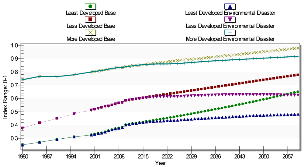
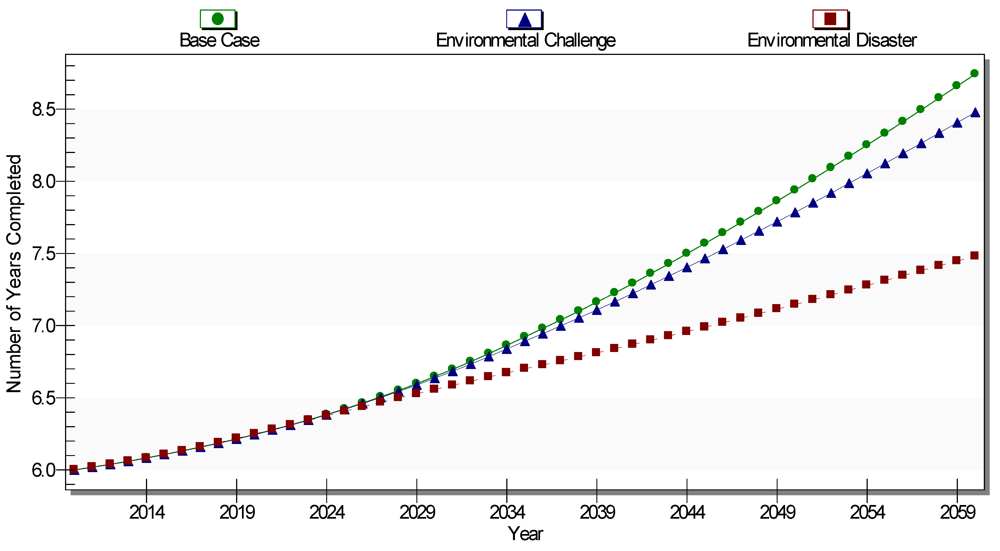
4.2. Drilling Down by HDI Component

Turning to the sub-dimensions of the HDI—long and healthy life (indicated by life expectancy), knowledge (as measured by mean years of schooling and expected years of schooling), and a decent standard of living (as measured by the log of GDP per capita at PPP)—the environmental impacts on development remain clear. With respect to life expectancy at birth, the difference in 2060 between the most extreme scenarios is seven years or about 10 percent. Global life expectancy in the Environmental Disaster scenario begins to decline after 2040. Again, the decline is primarily concentrated among less developed countries; more developed countries continue to slowly gain life expectancy and that of the least developed countries is, on average, mostly flat.

The global pattern across scenarios for average years of formal education (adults age 25 and older) may surprise some readers (see Figure 5). Figure 5 shows the values for the three scenarios, focusing only on the less developed countries, the set that we have seen to be especially vulnerable to environmental challenges in absolute terms (while the least developed are especially vulnerable in relative terms). In this case the years of education continue to grow even in the Environmental Disaster scenario. Why? Because years of education is an asset for an aging population. The flow of young people who are now, at least in historically relative terms, “pouring” out of primary and secondary schools around the world is replacing elderly cohorts that had very little education. That is, the upward march of average years of education has a great deal of momentum even should the flow out of school stabilize or decline somewhat.

Figure 5. Average years of education of adults in less developed countries across environmental scenarios.

Figure 5. Average years of education of adults in less developed countries across environmental scenarios.

Global income across the alternative scenarios is a rather sad story. Even in the Base Case the current gap between more and least developed countries is obviously much more dramatic than for either life expectancy or years of education. Specifically, it is nearly $24,000 at purchasing power, a factor of about 22. In the Base Case forecast the absolute gap grows to $64,000 but the ratio declines to a factor of less than 9. The good news of the Base Case, in spite of the large gaps, is that GDP per capita for the least developed countries grows from about $1,100 to more than $8,000 in 2060. But in Environmental Disaster the GDP per capita for the least developed countries rises to only $1,900. The ratio of income in more and least developed countries ends at more than 20, not very different than the current one.

5. Conclusions

As measured by the Human Development Index [43], the rapid pace of advances in human development of the last several decades will almost certainly slow around the world in coming decades. The mechanical aspects of the index’s construction, including the built-in saturation effects, will assure that. Notwithstanding those effects, and in spite of some important environmental constraints already represented within it, the HDI in the Base Case of IFs climbs quite significantly. By 2060 the world as a whole might add about 0.17 points to the current value, which is about the same as has been added in the last 30 years. The least developed countries, both due to their lower starting points (and therefore less saturation effect), and because of their more rapid growth on all dimensions of the index, could add nearly 0.25 points. Thus, both human well-being and equity improve.

Environmental constraints including climate change could, however, threaten such progress in part or almost in total. The Environmental Challenge scenario still allows the HDI to rise globally and across all income categories, which is good news, but dramatically reduces the size of the gains and very significantly slows the movement towards global equity. The Environmental Disaster scenario almost stops progress on the index everywhere. One major exception is the knowledge component, notably the indicator of average years of adult education, which has a great deal of built-in momentum because of the demographic replacement over time of poorly educated elderly populations with much more highly educated contemporary youth. The global HDI could be nearly 0.15 points lower in 2060 than in the Base Case; least developed countries, with dramatically lower levels already, could suffer a loss from the Base Case potential of nearly 0.17 points.

Fortunately, Environmental Disaster has a low probability, at least over the time horizon of this analysis. From a pessimistic perspective that is of little consolation because the stock constraints stemming from environmental problems (decreasing fossil fuel availability, falling water tables, rising atmospheric carbon and temperatures, and much more) are likely to keep growing well beyond 2060. From an optimistic point of view, the stocks of human resourcefulness (education levels, accumulated knowledge, and capital stocks) are also likely to continue growing. It is largely because of those that the Environmental Disaster scenario explored here did not lead to a Malthusian or Limits to Growth-like collapse in IFs forecasts, but rather to a dramatic slowdown in the advancement of human well-being and something of a stand-off between the two sets of forces. That kind of uneasy stability would, of course, most likely not persist for long.

References and Notes

1. Toynbee, A. A Study of History; Weathervane Books: New York, NY, USA, 1972. [Google Scholar]
2. Tainter, J.A. The Collapse of Complex Societies; Cambridge University Press: Cambridge, UK, 1988. [Google Scholar]
3. Diamond, J. Collapse: How Societies Choose to Fail or Succeed; Viking: New York, NY, USA, 2005. [Google Scholar]
4. Rochström, J.; Steffan, W.; Noone, K.; Persson, Å.; Chapin, F.S., III.; Lambin, E.; Lenton, T.M.; Scheffer, M.; Folke, C.; Schellhuber, H.J.; et al. Planetary Boundaries: Exploring the Safe Operating Space for Humanity. Ecol. Soc. 2009, 14, p. 32. Available online: http://www.ecologyandsociety.org/vol14/iss2/art32/ (accessed on 7 May 2012).
5. The Frederick S. Pardee Center for International Futures provides the foundational funding of the IFs project. The Center’s flagship project is a series of volumes on Patterns of Potential Human Progress (http://www.ifs.du.edu/documents/index.aspx). During 2000–2003, development of International Futures was funded in substantial part by the TERRA project of the European Commission and by the Strategic Assessments Group of the U.S. Central Intelligence Agency. In more recent years funding was provided by the U.S. National Intelligence Council in support of its global trends analyses (for 2020, 2025, and 2030), and by the United Nations Environment Programme for its Global Environment Outlook 4. None of these institutions bears any responsibility for the analysis presented here, but their support has been greatly appreciated. Thanks also to the National Science Foundation, the Cleveland Foundation, the Exxon Education Foundation, the Kettering Family Foundation, the Pacific Cultural Foundation, the United States Institute of Peace, General Motors and the RAND Pardee Center for funding that contributed to earlier generations of IFs. Also of great importance, IFs owes much to the large number of students, instructors, and analysts who have used the system over many years and provided much appreciated advice for enhancement.
6. Hughes, B.B.; Johnston, P.D. Sustainable futures: Building policy options into a scenario for development in a global knowledge society. Futures 2005, 37, 813–831. [Google Scholar] [CrossRef]
7. Moyer, J.D.; Hughes, B.B. ICTs: Do they contribute to climate change or sustainable development? Technol. Forecast. Soc. Change 2012, in press.. [Google Scholar]
8. United States National Intelligence Council (NIC), Mapping the Global Future; USGPO: Washington, DC, USA, 2004.
9. United States National Intelligence Council (NIC), Global Trends 2025: A Transformed World; USGPO: Washington, DC, USA, 2008.
10. United Nations Environment Programme (UNEP), Global Environment Outlook 4; UNEP: Nairobi, Kenya, 2007.
11. Available online: www.ifs.du.edu/ifs (accessed on 7 May 2012). The IFs model, help system, and related materials.
12. Wigley, T.M.L. IFs calculates country-specific temperature and precipitation change based on results aggregated from grid-level data produced by the MAGICC model. MAGICC/SCENGEN 5.3: User Manual (version 2); National Center for Atmospheric Research: Boulder, CO, USA, 2008. Available online: http://www.cgd.ucar.edu/cas/wigley/magicc/UserMan5.3.v2.pdf (accessed on 7 May 2012). In combination with estimates of carbon fertilization, these data are used to calculate a change in agricultural yields relative to 1990 levels. Absolute agricultural production declines are mitigated as price signals help more land to be placed under cultivation and more food to be traded..
13. Solow, R.M. We’d Better Watch out. New York Times Book Review; New York, NY, USA, 12 July 1987; p. 36. Available online: http://www.standupeconomist.com/pdf/misc/solow-computer-productivity.pdf (accessed on 7 May 2012).
14. Crafts, N. The Solow Productivity Paradox in Historical Perspective. London School of Economics, London, UK, 2001. Available online: http://www.j-bradford-delong.net/articles_of_the_month/pdf/Newsolow.pdf (accessed on 7 May 2012).
15. Sachs, J.D.; Warner, A.M. Economic Convergence and Economic Policies; Working Paper No. 5039; NBER: Cambridge, MA, USA, 1995. Available online: http://www.nber.org/papers/w5039 (accessed on 7 May 2012).
16. Collier, P. Geography and Growth. Oxford University, Department of Economics, Centre for the Study of African Economies, Oxford, UK, 2006 (Revised August). Available online: http://eiti.org/UserFiles/File/collier_africa_geography_growth.pdf (accessed on 7 May 2012).
17. Fukuda-Parr, S. The Human Poverty Index: A multidimensional measure. Poverty Focus 2006, 7–9. [Google Scholar]
18. Busby, J.W.; Smith, T.G.; White, K.L.; Strange, S.M. Locating Climate Insecurity: Where Are the Most Vulnerable Places in Africa? Working Paper; The Robert S. Strauss Center Climate Change and African Political Stability: Austin, TX, USA, 2010. [Google Scholar]
19. Hubbert, M.K. Energy from Fossil Fuels. Science. 1949, 109, pp. 103–109. Available online: http://www.hubbertpeak.com/hubbert/science1949/ (accessed on 7 May 2012).
20. United States General Accountability Office. Crude Oil: Uncertainty About Future Oil Supply Makes it Important to Develop a Strategy for Addressing a Peak and Decline in Oil Production; GAO-07-283; GAO: Washington, DC, USA, 2007. Available online: http://www.gao.gov/new.items/d07283.pdf (accessed on 7 May 2012).
21. Colin Campbell and others at the Association for the study of Peak Oil & Gas are among those who argue we have reached the peak of global oil production. Available online: http://www.peakoil.net (accessed on 7 May 2012).
22. In particular, IFs does constrain the advance of renewable energy, which in the base case grows quite rapidly, by the growing needs for electric-grid infrastructure or power storage that will need to accompany an alternative energy system if it is heavily dependent on new renewable forms.
23. Available online: http://www.businessinsider.com/the-impact-of-oil-prices-on-economic-growth-2011-2) (accessed on 7 May 2012). As cited by David Wessel, economic editor of The Wall Street Journal (see http://www.npr.org/2011/03/31/135002308/economy-update). This is an uncertain relationship subject to controversy and an alternative generalized rule is that the effect is 0.5 percent. Dean Baker of the Center for Economic and Policy Research explores this second generalized rule and suggests that the effect might be only half as great, closer to the assessment of Wessel.
24. They did not determine boundaries for chemical pollution and atmospheric aerosol loading.
25. The lack of data on the ultimate availability of groundwater reserves is a constraint to our modeling in this area.
26. World Population to reach 10 billion by 2100 if Fertility in all Countries Converges to Replacement Level. Available online: http://esa.un.org/unpd/wpp/Other-Information/Press_Release_WPP2010.pdf (accessed on 7 May 2012).
27. Homer-Dixon, T.F. Environment, Scarcity, and Violence; Princeton University Press: Princeton, NJ, USA, 1999. [Google Scholar]
28. Raleigh, C.; Urdal, H. Climate change, environmental degradation and armed conflict. Polit. Geogr. 2007, 26, pp. 627–638. Available online: http://linkinghub.elsevier.com/retrieve/pii/S0962629807000856 (accessed on 7 May 2012).
29. Taleb, N.N. The Black Swan; Penguin: New York, NY, USA, 2007. [Google Scholar]
30. Garrett, L. The challenge of global health. Foreign Aff. 2007, 86, 14–38. [Google Scholar]
31. Hughes, B.B.; Kuhn, R.; Peterson, C.M.; Rothman, D.S.; Solórzano, J.R. Improving Global Health; Paradigm Publishers: Boulder, CO, USA; Oxford University Press: New Delhi, India, 2011; Patterns of Potential Human Progress Series Volume 3. [Google Scholar]
32. Hughes, B.B.; Kuhn, R.; Peterson, C.M.; Rothman, D.S.; Solórzano, J.R.; Mathers, C.D.; Dickson, J.R. Projections of global health outcomes from 2005 to 2060 using the international futures integrated forecasting model. Bull. World Health Org. 2011, 89, 469–544. [Google Scholar] [CrossRef]
33. Mathers, C.D.; Loncar, D. Projections of global mortality and burden of disease from 2002 to 2030. PLoS Med. 2006, 3, p. e442. Available online: http://www.plosmedicine.org/article/info:doi/10.1371/journal.pmed.0030442 (accessed on 7 May 2012).
34. Mathers, C.D.; Loncar, D. New projections of global mortality and burden of disease from 2002 to 2030. PLoS Med. 2006, 3. Available online: http://www.biomedsearch.com/attachments/00/17/13/20/17132052/pmed.0030442.sd004.pdf (accessed on 7 May 2012). Protocol S1 Technical Appendix to Mathers and Loncar 2006..
35. Ezzati, M.; VanderHoorn, S.; Lopez, A.D.; Danaei, G.; Rodgers, A.; Mathers, C.D.; Murray, C.J.L. Comparative quantification of mortality and burden of disease attributable to selected risk factors. Global Burden of Disease and Risk Factors. Lopez, A.D., Mathers, C.D., Ezzati, M., Jamison, D.T., Murray, C.J.L., Eds.; 2006, pp. 241–396. Available online: http://www.dcp2.org/pubs/GBD (accessed on 7 May 2012).
36. Available online: http://www.ifs.du.edu.
37. Hughes, B.B.; Irfan, M.T.; Moyer, J.D.; Rothman, D.S.; Solórzano, J.B. Forecasting the Impacts of Environmental Constraints on Human Development; Human Development Reports Research Paper 2011/8; UNDP: New York, NY, USA, 2011. Available online: http://hdr.undp.org/en/reports/global/hdr2011/papers/HDRP_2011_08.pdf (accessed on 7 May 2012).
38. Hughes, B.B.; Irfan, M.T.; Khan, H.; Kumar, K.; Rothman, D.S.; Solórzano, J.R. Reducing Global Poverty; Paradigm Publishers: Boulder, CO, USA; Oxford University Press: New Delhi, India, 2009; Patterns of Potential Human Progress Series Volume 1. [Google Scholar]
39. Dickson, J.R.; Hughes, B.B.; Irfan, M.T. Advancing Global Education; Paradigm Publishers: Boulder, CO, USA; Oxford University Press: New Delhi, India, 2009; Patterns of Potential Human Progress Series Volume 2. [Google Scholar]
40. United Nations Human Development Programme, The Real Wealth of Nations: Pathways to Human Development; Human Development Report 2010; Palgrave Macmillan: New York, NY, USA, 2010.
41. Although the official measure uses Gross National Income (GNI), the IFs system uses the very nearly identical GDP.
42. The values shown here will differ slightly from those we provided for the 2011 Human Development Report (UNDP 2011) because we have created them with a somewhat later version of the IFs system. Among the differences between that version and earlier ones is the movement of the model to a 2010 base year. There are small transients between historical values and those of IFs in the base year because the values IFs computes for all of the inputs of the HDI vary somewhat from those used by the UN Human Development Report Office.
43. Neumayer, E. The human development index and sustainability—A constructive proposal. Ecol. Econ. 2001, 39, 101–114, We have recognized throughout that the HDI is not a general measure of human progress, but one more narrowly focused on human development. It has been criticized for various reasons, including not considering issues of sustainability. See also Sagar, A.D.; Najam, A. The human development index: A critical review. Ecol. Econ. 1998, 25, 249–264. It also fails to recognize the potential validity of alternative cultural perspectives on human well-being.. [Google Scholar]
44. United Nations Development Programme. Human Development Report: Sustainability and Equity: A Better Future for All; Palgrave Macmillan: New York, NY, USA, 2011. Available online: http://hdr.undp.org/en/reports/global/hdr2011/ (accessed on 7 May 2012).
Appendix
Section 2 of the paper identified the basic models integrated into the International Futures (IFs) system and listed some of the components within each. This appendix provides the key equations of the models related to the paper, explains the computational sequence, and gives basic information concerning the supporting database and parameterization of the models. Those users who wish additional information should turn to the Help system that is integrated with both the on-line and stand-alone versions of IFs (at http://www.ifs.du.edu/ifs/index.aspx) and explore the documents of the project, both working reports and publications (at http://www.ifs.du.edu/).
Each of the models within the IFs system is very large, generally comparable in character and structure to the most substantial models in their respective issue areas at institutions such as the United Nations Population Division (population forecasting), the World Bank (economic forecasting), the International Institute for Applied Systems Analysis (education forecasting), the World Health Organization (health forecasting), and so on. We therefore must be selective here with respect to documentation.
The model structure is recursive (sequential computation of each equation in every annual time step) rather than relying upon simultaneous or iterative within-year solution procedures. Much attention is paid to maintaining accounting identities, including (1) those around global production, consumption, and trade of food categories (crops and meat) and of energy types (oil, natural gas, coal, hydropower, nuclear power, and new renewables), both in physical and value terms; and (2) those involving inter-sectoral flows and inter-agent (households, firms, and governments) flows nationally and internationally, in value terms. Because the model's orientation is long-term forecasting, it is also important that it track stocks (accumulations such as the growth of atmospheric carbon and the decline of fossil fuel resource bases) as well as annual flows; yet the model structure is not systems dynamics in form, but rather a hybrid involving also many econometrically estimated specifications. Further, its long-term character and its integration of multiple issue areas means that specifications of algorithmic structures (such as endogenization of multifactor productivity driven by human, social, physical, and natural capital elements) can become as important as equations. All of this is to explain that the equations below are only a part of the overall system.
Sequencing of equations for recursive solution frequently involves moving out of one major model (e.g., population) into another (e.g., economics) and then later back again to earlier models. The sequencing is actually somewhat different in the first year of the model’s computation, when many variables are initialized, than in all subsequent years. And we should point out that, prior to the first or base year of computation (currently 2010) the system relies on an extensive “pre-processor” of data for all its models, reconciling (again often with algorithms) physical and value estimates that are often incompatible and filling holes in data for the system’s 183 countries (often using cross-sectional formulations tied to income levels). We focus here, however, only on the annual computations for years after the initialization.
Notation explanation. In the equations that follow we show variable names (explained in the text) in capital letters and parameters in lower case. We use bold face to represent values exogenous to the system, namely initial conditions of variables (from data) or parameters. The subscript “r” refers to geographic region, which in IFs is almost always a country (the model now represents 183 countries). Second subscripts represent additional dimensionality (s for economic sector, f for food type, e for energy type, g for government spending sector). The superscript “t” refers to the current time step; “t-1” to a variable computed in a previous time step and carried forward; and “t=1” to initial conditions.
Population and Economic foundations. The first calculations are of basic variables in what are essentially the two core models of the IFs system (see again Figure 1 of the article). In the demographic model we draw heavily upon the age-sex population distributions and other variables computed at the end of the previous time step to compute population (simply a sum across the age distribution), population growth, median age, HIV rate, AIDs deaths, calorie demands, sub-populations of importance (e.g., the size of the working-age population), and household-size. In the economic model, again using variables from previous years that we will explain below, we compute, inter alia, labor supply, female share of labor, exogenous technological growth, human capital, social capital, physical capital, knowledge capital, and productivity growth.
Agriculture. We then use such basic variables as important drivers for demand and supply sides in the physical models of the system, namely agriculture and energy, as well as a few infrastructure variables that we omit here because of more substantial treatment later (in interaction with variables in each of these models that also carry over from past years). Turning first to agricultural production, crop and meat/fish supply have very different bases and IFs determines them in separate procedures. Crop production depends on yields per hectare of land under cultivation and on the amount of land cultivated. Yield functions are almost invariably some kind of saturating exponential which represents decreasing marginal returns on inputs such as fertilizer or farm machinery. IFs also uses a saturating exponential, but imposes it on a Cobb‑Douglas form. The Cobb-­Douglas function is used in part to maintain symmetry with the economic submodel but more fundamentally to introduce labor as a factor of production along with capital. Especially in less developed countries (LDCs) where a rural labor surplus exists, there is little question that labor, and especially labor efficiency improvement, can be an important production factor. “Know‑how” is also important in agriculture and there is therefore a technology term.
IFs computes yield in two stages. The first provides a basic yield (BYL) representing change in long‑term factors such as capital and labor. The second stage uses this basic yield as an input and modifies it based on prices and therefore on the representation over time of the supply-demand equilibrium.
The basic yield (BYL) requires capital in agriculture (KAG), labor (LABS), technological advance (AGTECH), a scaling parameter (CD), and an exponent (CDALF). In addition a saturation coefficient (SATK) introduces the behavior of the saturating exponential. Interpret AGTECH as a factor-neutral technological progress coefficient.
Sustainability 04 00958 i001
The saturation coefficient is a multiplier of the Cobb‑Douglas function. It is the ratio of the gap between an exogenously specified maximum possible yield and the most recently computed yield to the gap between the maximum yield and the initial yield, raised to an exogenous yield exponent. With positive parameters the form produces decreasing marginal returns.
The basic yield represents the long‑term tendency in yield but, because agricultural production levels are quite responsive to short–term factors such as fertilizer use levels and intensity of cultivation, the annual yield will vary significantly around that tendency. Those short-term factors under farmer control (therefore excluding weather) depend in turn on prices, or more specifically on the profit (FPROFITR) that the farmer expects. Because of computational sequence, we use food stocks as a proxy for profit level and adjust basic yield accordingly.
There are, however, additional factors that can influence agricultural yield. The one of importance to us here is global climate change. IFs therefore recomputes yield (YL), modifying it by two multipliers. The first summarizes the impact on yield of changes in precipitation and temperature resulting from global levels of atmospheric carbon (ENVYLCHG); we lag that variable from the previous time step and will see its computation near the end of this appendix. The second factor is a regional yield multiplier (ylm) that allows the model user to introduce assumptions about weather patterns and other uncertain elements in the agricultural system.
Sustainability 04 00958 i002
Finally, agricultural production (AGP) in the first or crop category is the product of yield and land devoted to crops (LD).
Sustainability 04 00958 i003
The production of fish has two components, ocean and mariculture. Total global ocean fish catch (OFSCTH) is set exogenously, as is each region’s share in it (RFSSH) and the regional value of aquaculture (AQUACUL). Livestock production (AGPLV) is dependent on the herd size (LVHERD) and the slaughter rate (SLR). Total fish and livestock production, food category two, is the sum. Some food production will never make it to markets, but will be lost in the field or in distribution systems to pests, spoilage, etc. That loss (LOSS) is a function of GDP per capita in a table function that captures the tendency of loss to decrease with higher income levels. A loss multiplier (LOSSM) allows scenario introduction.
Energy. Basic total energy demand (BENDEM) for a given region or country is tied very closely to gross domestic product (GDP). IFs actually uses GDP from a previous time cycle (with an estimate of growth) because the recursive structure of IFs computes current GDP later.
The units of energy required for every unit of gross domestic product (ENDK) are a function of GDP per capita in purchasing power terms (GDPPCP), computed in a table function.
Sustainability 04 00958 i004
Initial data from countries/regions are unlikely to fall exactly on this table function initially. To reconcile computed energy demand (ENDEM) in the first year with empirical demand, IFs computes an internal adjustment multiplier (ENDM),which relies in turn on energy demand the first year; initial energy demand is apparent consumption computed from the sum across types of energy production (ENP) plus imports (ENM) minus exports (ENX).
Sustainability 04 00958 i005
Final energy demand (ENDEM) is a price-responsive function of this basic energy demand. Possible tax on the consumer’s price added by carbon taxes (cartaxenpriadd) is added to the basic market price. In an earlier version of the submodel, we used a smoothed or moving-average, regionally-specific energy price (SENPRI) relative to the initial price value (ENPRI). Because energy is a quite highly integrated global market, and in order to enhance behavioral stability, we have gone to using the world energy price (lagged one year) relative to initial price; prices affect demand through an elasticity (elasde). The user can force change in energy demand directly via an energy demand multiplier (endemm).
Sustainability 04 00958 i006
The basic computation of energy production (ENP) uses only capital as a factor or production. Energy production is the quotient of capital in each energy category (KEN) and the appropriate capital-to-output ratio (QE). The model user can modify a multiplier to this ratio (QEM) to represent changes in technology. The capital-to-output ratio is itself a function of resource availability. E Known reserves (RESER) pose a direct con­straint on production; they are constrained by ultimate resource assumptions in an important process not described here. The reserve-to-production ratio may not fall below a specified factor (PRODTF). In the case of oil and gas, for example, no more than about 10% of known reserves can be produced in a given year. Within the reserve constraint, the user can force increases or decreases in production via an energy production multiplier (ENPM). A capacity utilization factor (CPUTF) also affects the production level and is computed dynamically over time to help maintain market equilibrium (as are prices).
Sustainability 04 00958 i007
Return to the Economic Model and Production. The physical flows of the partial equilibrium models for energy and agriculture, along with the change over time in relative prices for those goods (computed in processes that equilibrate the global market but also represent changing production cost fundamentals), provide inputs to two of the six sectors in the economic model (those six being agriculture, energy, other raw materials, manufactures, energy, and information and communications technology). They can therefore next be integrated with more value-based computations for the other sectors in the important production side of the economic model.
A Cobb-Douglas function produces value added (VADD) as a function of capital (KS) and labor (LABS), a cumulative technological growth factor (TEF), and a scaling parameter (CDA) computed in the first time step. The capital exponent CDALFS) and its labor complement are endogenous, and the capital share declines with GDP per capita [1].
Sustainability 04 00958 i008
The annual growth rate in multifactor productivity (MFPGRO) requires, of course, further explanation. As discussed above, there is a base rate (MPRATE) linked to systemic technology advance and a convergence premium. Specifically, the base rate sums the exogenously specified rate of advance in the leader (mfpleadr) and the premium computed for convergence of each country/region (MFPPrem), a function of GDP per capita at purchasing power parity (GDPPCP).
Sustainability 04 00958 i009
On top of the base rate, multiple (currently four) terms additively affect/shift growth over time, each comparing country performance with structural expectations [2]. The model computes an adjustment or correction factor (MFPCOR) in the first year so as to make the overall growth rate initially consistent with recent historical experience for the country.
Turning to the four clusters of drivers discussed above, we discuss the human capital term illustratively. The annual change in MFP attributable to education (CNGEDUC) is the sum of two terms. The first compares the endogenous computation of average years of education (EDYRSAG25) of the population at age 25 or older (responsive to all of the factors represented in the education module) minus the expected value of the same variable computed from a cross-sectional function (EXPECTEDEDYRSAG25). The second term similarly compares the portion of the GDP that government directs to education (g=EDUC) with the expected value of the same ratio. The contribution to the human capital from health is directly comparable. Four parameters from the literature (in bold face) convert differences from expected values into shifts of productivity growth.
Sustainability 04 00958 i010
Often across the IFs system, we estimate our own parameters from our database of over 2,000 series across the multiple issue areas. But in many critical areas, especially those in which there are large literatures, we draw from those literatures so as to incorporate expertise that ranges far beyond our own. Hughes [3] described the parameterization of the production system, drawn from an extensive literature of estimations and stylized facts on productivity [4]. Illustratively, parameterization considered years of education and educational expenditures as a pair. Analyses in the literature include:
• Barro and Sala-i-Martin [5] reported that a 1 standard deviation increase in male secondary education raised economic growth by 1.1% per year, and a 1 standard deviation increase in male higher education raised it by 0.5%. Barro [6] reported that one extra year of male upper-level education raised growth by 1.2% per year.
• Chen and Dahlman [7] concluded that a rise of 20% in average years of schooling raises annual growth by 0.15 percent and that an increase in average years by 1 year raises growth by 0.11 percent.
• Jamison, Lau, and Wang [8] used the Barro-Lee measure of average years of school for males between 15 and 60, but concluded that the “effect was small”.
• Bosworth and Collins [9] argued that each year of additional education adds about 0.3% to annual growth.
• The OECD [10] found that one additional year of education (about a 10% rise in human capital) raised GDP/capita in the long run by 4–7%.
• Barro and Sala-i-Martin [5] concluded that increasing education spending as a portion of GDP by 1.5 points (one standard deviation) raised growth by 0.3%.
• Baldacci, Clements, Gupta, and Cui [11] found that raising education spending in developing countries by 1% a year and keeping it higher added about 0.5% per year to growth rates. They also found that 2/3 of the effect of higher spending is felt within 54 years but the full impact shows up only over 10–15 years.
Gross regional or domestic product (GDP) is simply the sum of value added across sectors, which would also equal the sum of production for final demand across sectors. And the GDP per capita (GDPPC) follows easily.
The basic GDP figures for the model are represented in dollars at official exchange rate values. It is important, however, to estimate the value of GDP and GDPPC at purchasing power parity levels as well (GDPP and GDPPCP). To do that we need to compute a purchasing power parity conversion value (PPPConV). Data sources provide the initial conversion value. IFs uses an analytic function based on GDP per capita to compute change in the conversion value over time.
Sustainability 04 00958 i011
Broader Financial Flows and the Social Accounting Matrix. The computational flow moves next to financial flows, beginning with computations of assorted international flows, including foreign direct investment (maintaining stocks over time as well as flows), portfolio investment, IMF and World Bank credits and loans, and worker remittances. As in many areas of the model, we do not, of course, expect to be able to forecast these with any reasonable accuracy for 183 countries over the long run. But they are important variables for which we can provide basic relationships, thereby also adding handles for users undertaking scenario analysis.
Turning to the domestic side of financial flows, and beginning with expenditures, Figure A.1 shows the function estimated cross-sectionally in order to fill the relatively few holes in government expenditures as a portion of GDP (using data from the World Development Indicators).
Government expenditures consist of a combination of direct consumption/expenditure and transfer payments. As a general rule, transfer payments grow with GDP per capita more rapidly than does consumption. And within transfer payments, pension payments are growing especially rapidly in many countries, particularly in more-economically developed ones.
In future years the total of government expenditures is calculated from the sum of direct consumption and transfers. The two components, however, each require a moderately complex calculation that we do not elaborate here. Computation of government consumption (direct expenditures on the military, education, health, R&D, foreign aid, and other categories) begins with use of the function to compute an estimated government consumption (EstGovtConsum) as a portion of GDP, using GDP per capita (PPP) as the driver. The initialization discussion above showed the empirical base of that function. It carries a behavioral assumption of generally increasing expenditures with increases in GDP per capita.
Figure A.1. Government Expenditure Share as Function of GDP/capita (PPP).
Sustainability 04 00958 g006
The estimated value then enters a convergence calculation that IFs uses in a number of instances. In the first year a ratio term (GovConR) was computed that represented the degree to which a country’s consumption/GDP differed from the estimated value. That ratio multiplies the estimated term in future years, allowing the function normally to increase consumption/GDP as GDP per capita rises. At the same time, such divergence from estimated functions is almost as often a matter of data inadequacy or of temporary factors for a country as it is of persistent idiosyncrasy. The convergence function allows the country/region’s value to converge towards the functional calculation over a period of time (govfinconv), usually quite long. Such convergence also helps avoid ceiling effects (e.g., government consumption as 100% of GDP) as GDP per capita rises.
The second term in the equation below is called the Wagner term, after the discoverer of the long-term behavioral tendency for government consumption to rise as a share of GDP, even at stabile levels of GDP per capita. This is built into the consumption calculation through an exogenous parameter (wagnerc) that is multiplied by the number of the forecast year.
Sustainability 04 00958 i012
Almost finally, government consumption is further modified by an exogenous multiplier of government expenditures, allowing the user to directly control it by country/region and by an endogenously computed multiplier on expenditures (MulExp) that reflects the balance or imbalance in government expenditures and the debt level. Finally, and not shown, there is a simple adjustment to reflect the effect that changing levels of foreign assistance receipts can have on consumption.
The division of government expenditures into target destination categories (GDS) is, of course, also a key agent-class behavior. We do not describe it in detail here, but it involves determining demand for military, health, education, R&D, infrastructure and a residual other category of expenditures from extended representations of the demand for all but R&D and the residual other category. Actual expenditures are normalized to total government consumption.
Governance. The IFs system represents a number of governance variables in the general categories of security, capacity, and inclusion. Here we illustrate just two. With respect to capacity, one of the most powerful measures of capacity (or more accurately, lack of capacity) may well be corruption. We rely in our analysis on the Transparency International measure of corruption perceptions, which in spite of the name they give it is actually a measure of transparency (higher values are more transparent or less corrupt). Note that the basic formulation in IFs for corruption/transparency (below) contains four drivers, all of which are significant, and which collectively explain nearly 80 percent of the cross-country variation in corruption in the most recent year of data for each variable. The first term, and the one that by itself explains the most variation, is a long-term development term, in this case GDP per capita (for some variables to be discussed below, such as democracy, that development variable is years of education).
Interestingly another very powerful term is the UNDP Gender Empowerment Measure (GEM), which, in spite of its high correlation with GDP per capita, makes its own contribution. A secondary term is the extent of democracy using the Polity scale (DEMOC). That this term makes an independent contribution to transparency suggests the power that inclusion may have to increase accountability and transparency, reducing corruption. An even-less-powerful but still-significant term is the dependence of the country on exports of energy (ENX) converted to value terms with prices (ENPRI)—in a few years, and in the aftermath of the Arab Spring beginning in 2011, it will be interesting to know if this term drops out of analyses of change in governance regime and character. A multiplier for scenario analysis is the only exogenous element added to the basic formulation (govcorruptm). This equation has an R-squared in 2010 of 0.76.
Sustainability 04 00958 i013
With respect to inclusion, we pay particular attention to regime type. As with capacity, the forecasting of regime type in IFs has multiple elements: (1) a basic statistical formulation tied to literature analysis and our own estimations; (2) a recognition of country-specific differences (tied in part to path dependencies); and (3) an algorithmic specification of a number of additional factors, including global waves and neighborhood effects.
Most analyses of democratization place much emphasis on a developmental variable such as GDP per capita. GDP per capita and adults’ years of education are very highly correlated across countries, and we found that, although the correlation of GDP per capita and democracy level is slightly higher than that of education years and democracy, when we added the size of the youth bulge and the extent of dependence on energy exports, the better broad developmental driving variable proved to be years of adults’ education. With additional exploration, however, we found a slight further advantage for the Gender Empowerment Measure, and so replaced the education variable with the GEM (which is, itself, strongly influenced by adults' education). In the equation below, the basic IFs formulation, all terms are significant with T-scores above 2.0 in absolute terms. In earlier work we also explored a linkage to the survival/self-expression dimension of the World Value Survey, but have found that other development variables statistically force it out of the relationship.
Sustainability 04 00958 i014
IFs has the capability of doing an historical simulation between 1960 and 2010 so that we can compare our forecasts with data. Our forthcoming governance volume [12] documents our use of that in order to build a broader forecasting structure on top of the basic equation above, as well as documenting the rest of the governance model. Governance variables enter the economic model primarily via the production function described above.
Agricultural Demand. Sequentially it could have been computed earlier (many of the IFs sequential steps could be changed), but agricultural demand is dependent on estimates of income. Crop demand has three components: feed, industrial and food. These equations are important but do not greatly affect the dynamics that surround analysis in this article, so we do not document them here.
Back to the Economy: But looking forward with investment. The determination of investment by destination that will carry changes in capital stock to the next time period is a two-step procedure. First, IFs computes demand for investment by each sector (IFSDEM), responsive primarily to inventory (or stock) levels. This is a reasonably extensive process involving the use of what engineers term a PID controller to feed back information from inventories (the integral of disequilibrium and annual change of inventories (the derivative term in PID) to the demand for investment funds.
More generally, a variety of PID controller mechanisms help the model in the chasing of equilibrium over time. These mechanisms show up in all price calculations (food and energy prices in the physical models and relative prices of all other sectors in the economic model), in determinations of interest rates for balancing savings and investments, and in determinination of exchange rates for relative currency values. It is typical to talk of alternative “closures” in describing economic models, that is the use of hard specification of supply or demand side variables to determine equilibrium. Our more open method of search for it with signals back to the supply and demand sides allows both exogenous interventions on both sides (related to the kinds of scenario specifications described in the article) and more elaborate specifications of both supply and demand sides, including the multiple linkages across models that this appendix has been describing.
Building Infrastructure. Here we compute many infrastructure demand and access variables including Road Density, Paved Roads, Rural Roads Access Index, Cost of adding a lane km of paved road, Land Area Equipped for Irrigation, Per Hectare Cost of equipping land for irrigation, Fixed Telephone Line density, Cost of adding a fixed land line, Access to Electricity Grid, Electricity Consumption, Electricity Transmission Loss, Electricity Generation Capacity, Electricity Generation Capacity Cost, Computers per 100 people, Access to Sanitation facilities, Cost of Sanitation, Access to Safe Water, Cost of Safe Water. We illustrate this with only one, electricity access.
Sustainability 04 00958 i015
where
INFRAELECACC is the percentage of the urban or rural population with access to electricity, poverty level is the fraction of the total population that lives on less than $1.25 per day, and GOVEFFECT is a measure of governance effectiveness developed as part of the World Bank’s World Governance Indicators project.
We recognize that there is a strong connection between the use of electricity and of solid fuels in the home. In general, as households move up the energy ladder, they increase their use of the former and decrease their use of the latter. We also include a link from access to electricity to the use of solid fuels in the home. This in turn enters the health model and affects the level of respiratory disease.
International Political Variables. We next compute a number of international political variables, including a power measure based on hard capabilities and an estimate of intra-dyadic threat. Those are not of great relevance to this article, so we do not elaborate them.
Population Dynamics. We are in a position at this point to compute a number of variables relevant to the dynamics of population over time. Although births, deaths, and migration all influence population dynamics, the most influential of the three is births. We therefore focus here on the critical variable, total fertility rate (TFR). IFs determines the TFR and then imposes that on the fertility distribution of the region/country.
Infant mortality (INFMOR), years of average education for those 15 and older (EDYRSAG15), and contraception use (CONTRUSE) are key drivers of fertility rates. In addition there is an exogenous multiplier on the rate (tfrm), and shift in that function with technological or cultural change (ttfrr).
Sustainability 04 00958 i016
Total fertility rate is, however, unlikely to shift indefinitely toward zero. In fact, it requires a value of about 2.0 simply to maintain a steady population (unless life expectancies are growing). TFR is therefore bound by a minimum that responds to a global parameter (tfrmin) normally set at either 1.5 or 1.8.
Once we have computed the total fertility rate (TFR), the number of births in a given year is a simple function of the fertility distribution and the TFR. On the mortality side, mortality patterns determine life expectancy and affect the progression of each age category through time. IFs includes an entire health model, based on work from the Global Burden of Disease project of the World Health Organization, but we do not need to document that here. We also compute other demographic variables of importance at this point including contraceptive use, births, deaths, infant mortality, crude birth rate, crude death rate, calories per capita, and malnourished children.
Other Human Development Variables. At this point we turn to the education model of IFs and compute expenditures per student, gross enrollment demand, graduates per level, years of education for people over 25 and for people over 15, and literacy.
Having computed economic, health, and education variables, we are able to compute also the Human Development Index (HDI) in the standard equation of the United Nations Human Development Report Office.
Other Variables, Indicators, and Forward Linkages. At this stage there are further calls to many of the models in IFs, some of them repeatedly, in order to calculate a wide range of variables that carry over to the next time step and of indicators of interest to model users. These include health variables such as smoking prevalence; smoking impact; BMI; obesity; mortality by country, age, gender and disease type; life expectancy; deaths per disease type; infant mortality; crude death rate; population growth rate; years of life lost; and years lost to disability. They also include: income-related variables such as household income per capita, domestic Gini, population living with income under $1.25/day and $2/day, poverty gap, household savings, firm savings, and global Gini; environmental variables such as urban pollution measured with PM2.5 levels, annual carbon emissions from fossil fuels, advanced sustainability analysis, precipitation change, temperature change, and agricultural yield change; agricultural variables such as return ratio on land/yield investment, investment in agriculture, urban built-up land development, crop land development, and grazing land development; knowledge system variables such as knowledge system index, knowledge human capital index, knowledge ICT index, knowledge innovation index, and knowledge international transfer index.
To illustrate some of special importance to this article, consider carbon emissions and the stock of atmospheric carbon. The beginning point for examining the greenhouse effect is calculation of the atmospheric carbon dioxide in parts per million (C02PPM). The model calculates annual emissions of carbon from energy use (CARANN) and adds it to a cumulative tracking of carbon (SACARB), initialized exogenously for 2010 (carint). Emissions depend on global production (WENP) in the fossil fuel categories (oil, gas and coal), using fuel-specific coefficients representing tons of carbon generated per barrel of oil equivalent burned (carfuel). The oceans and other sinks annually absorb an exogenously specified amount of atmospheric carbon (carabr) and that retards the accumulation. Deforestation (or reforestation) has an impact via another parameter (carforst).
Sustainability 04 00958 i017
We use a table function (based on figures from the IPCC) to determine the average world temperature (WTEMP) in Centigrade from the atmospheric carbon dioxide level in parts per million.
Sustainability 04 00958 i018
Given forecasts of global temperature change over time we are able to compute temperature and precipitation changes post 1990 for each country (TEMPCHG and PRECHG) using data compiled for the MAGICC/SCENGEN climate model [13]. Building on work by Cline [14] and Rosenzweig and Igelesias [15] we then estimate a variable that combines the effects of those variables with carbon fertilization into a multiplier on agricultural yield resulting from environment (ENVYLCHG). We saw earlier the impact of this on yields.
Conclusion. As we indicated at the beginning of this appendix, the IFs modeling system is a compilation of many very large individual models. As a result, it is impossible to provide full detail here. We have tried, instead, to indicate the key equations related to this article, the overall dynamics of annual computations, the roots of the system in an extensive database, and the widespread reliance on the expertise of others to structure the models, their equations and our parameterization. We welcome inquiries for more information.
1. Estimation of the relationship for capital share uses Global Trade and Analysis Project (GTAP) data, as do a number of other aspects of the model. For instance, the input-output matrices and factor.
2. Not shown, there is also an exogenous additive parameter (mfpadd) allowing users to intervene and change growth paths for any country/region. The presentation of equations here omits a number of such “exogenous handle” parameters and terms not central to the exposition.
3. Hughes, B.B. Productivity in IFs. Pardee Center for International Futures, University of Denver, Denver, CO, USA, 2005. Available online: http://www.ifs.du.edu/documents/reports.aspx (accessed on 7 May 2012).
4. Mankiw, Romer and Weil (1992) was one of the early extensive empirical analyses of growth. They found that the Solow model was generally correct and useful, but that a CES formulation improved performance. We stay here with the Cobb-Douglas version because it is so widely used. They also found that human capital accumulation, which they tapped with secondary school enrollment was very important and that OECD countries behaved differently than low income ones.
5. Barro, R.; Sala-i-Martin, X. Economic Growth; MIT Press: Ipswich, MA, USA, 1999; p. 431. [Google Scholar]
6. Barro, R.J. Inequality, Growth, and Investment; NBER Working Paper No. w7038; National Bureau of Economic Research: Cambridge, MA, USA, 1999; pp. 19–20. Available online: http://ssrn.com/abstract=156688 (accessed on 9 May 2012).
7. Chen, D.H.C.; Dahlman, C.J. Knowledge and Development: A Cross-Section Approach; World Bank Policy Research Working Paper No. 3366; World Bank: Washington, DC, USA, 2004. Available online: http:// papers.ssrn.com/sol3/papers.cfm?abstract_id=616107 (accessed on 9 May 2012).
8. Jamison, D.; Lau, L.; Wang, J. Health’s Contribution to Economic Growth in an Environment of Partially Endogenous Technical Progress. In Health and Economic Growth: Findings and Policy Implications; Lopez-Casanovas, G., Rivera, B., Currais, L., Eds.; MIT Press: Cambridge, MA, USA, 2005; p. 82. [Google Scholar]
9. Bosworth, B.P.; Collins, S.M. The empirics of growth: An update; Brookings Papers on Economic Activity. 2003, p. 17. Available online: http://www.brookings.edu/~/media/Files/rc/papers/2003/0922globaleconomics_bosworth/20030307.pdf (accessed on 9 May 2012).
10. Organisation for Economic Co-operation and Development (OECD), The Sources of Economic Growth; OECD: Paris, France, 2003; pp. 76–78.
11. Baldacci, E.; Clements, B.; Gupta, S.; Cui, Q. Social Spending, Human Capital, and Growth in Developing Countries: Implications for Achieving the MDGs; IMF Working Paper 04/217; International Monetary Fund: Washington, DC, USA, 2004; p. 24. [Google Scholar]
12. Hughes, B.; Joshi, D.; Moyer, J.; Sisk, T.; Solórzano, J. Strengthening Global Governance; Paradigm Publishers: Boulder, CO, USA; Oxford University Press: New Delhi, India, 2013; in press. [Google Scholar]
13. Wigley, T.M.L. MAGICC/SCENGEN 5.3: User Manual (version 2); National Center for Atmospheric Research: Boulder, CO, USA, 2008. Available online: http://www.cgd.ucar.edu/cas/wigley/magicc/UserMan5.3.v2.pdf (accessed on 7 May 2012).
14. Cline, W. Global Warming and Agriculture: Impact Estimates by Country; Peterson Institute for International Economics: Washington, DC, USA, 2007. [Google Scholar]
15. Rosenzweig, C.; Iglesias, A. Potential Impacts of Climate Change on World Food Supply: Data Sets from a Major Crop Modeling Study; Columbia University, Center for International Earth Science Information Network: New York, NY, USA, 2006. [Google Scholar]
Supplementary Files
• Supplementary File 1::
PDF-Document (PDF, 263 KB)
• Share and Cite
MDPI and ACS Style
Hughes, B.B.; Irfan, M.T.; Moyer, J.D.; Rothman, D.S.; Solórzano, J.R. Exploring Future Impacts of Environmental Constraints on Human Development. Sustainability 2012, 4, 958-994. https://doi.org/10.3390/su4050958
AMA Style
Hughes BB, Irfan MT, Moyer JD, Rothman DS, Solórzano JR. Exploring Future Impacts of Environmental Constraints on Human Development. Sustainability. 2012; 4(5):958-994. https://doi.org/10.3390/su4050958
Chicago/Turabian Style
Hughes, Barry B., Mohammod T. Irfan, Jonathan D. Moyer, Dale S. Rothman, and José R. Solórzano. 2012. "Exploring Future Impacts of Environmental Constraints on Human Development" Sustainability 4, no. 5: 958-994. https://doi.org/10.3390/su4050958
Article Metrics
Back to TopTop