Article

Ecology in Urban Planning: Mitigating the Environmental Damage of Municipal Solid Waste

by
Mindaugas Staniunas
1,
Marija Burinskiene
1 and
Vida Maliene
2,*
1
Department of Urban Engineering, Vilnius Gediminas Technical University, Vilnius 10223, Lithuania
2
School of the Built Environment, Liverpool John Moores University, Liverpool L3 3AF, UK
*
Author to whom correspondence should be addressed.
Sustainability 2012, 4(9), 1966-1983; https://doi.org/10.3390/su4091966
Submission received: 25 July 2012 / Revised: 9 August 2012 / Accepted: 17 August 2012 / Published: 24 August 2012

Abstract

:
The principles of well-known indices of sustainability—the Ecological Footprint (EF) and the Environmental Sustainability Index (ESI)—have been compared to discuss the essence of attitude, substantial differences and transferability into urban planning. An overview indicates that ideologically the EF is a more appropriate tool for ecological tasks due to its clear background of natural limits and the ability of “leakage” tracing. Furthermore the European Common Initiative is discussed as it proposes feasible indices monitoring actions towards local sustainability that could be considered in urban planning. Taking two Lithuanian cities as an example, integration of part of one index (regarding municipal solid wastes) into the ecological section of urban planning is presented. It has been estimated that in 10 years an average Lithuanian should generate an amount of municipal solid waste whose ecological impact will be equal to 19,900 kg of CO2-eq in 20 years time. Lastly considering urban planning scope and the EF practice, two opportunities are discussed: (1) tree planting and (2) waste incineration.

1. Introduction

Sustainability, defined in the proceedings of the Brundtland Commission, motivated experts to search for a way to estimate and assess new ideology, whilst politicians felt concerned about incorporating sustainability into policy and about its practical implementation. Theoretically, sustainability had to be achieved by establishing equilibrium between economics, social development and environment, inter alia avoiding sharp imbalance. However, more than 20 years passed but sustainable development was not realized anywhere [1]. Unsuccessful attempts remain as motivation to keep on trying and thus various methodologies have been developed and numerous different sustainability indices of countries, regions or cities have already been published [2,3]. Obviously, any calculation relies on some prime indicators, but as science develops over time the list of indicators is constantly updated and becoming longer. Whatever the method is, it has a scientific origin and has exponents, but the truth is that not always all results coincide with each other. Hence, there is a plethora of theories but no sustainability.
The European Union is firmly committed to sustainable development; it is a key principle for policies and actions [4]. According to European statistics, “in the European Union, 74% of the total population lives in cities and towns with more than 5000 inhabitants; in other words, only a quarter of all European citizens live in a rural environment” [5]. Therefore, urban sustainability or sustainable cities are supposed to be a kind of expectation for the majority of Europeans. The well-known way of achieving sustainability in cities is simple–an adequate planning policy and its implementation. The problem is that “adequate” implies a large and comprehensive scale; the following must be taken into consideration: economics, social development and the environment. This article is intended to investigate urban planning and sustainability with a slightly different approach. Despite intermingling the above-mentioned issues in the manner of sustainability, the central attention is to be placed only on the environment (ecology), for it is certainly true that the environment has limits while economics and social well-being do not. However, “ecology” itself seems to have a common and self-explanatory definition, yet it is not always able to reveal the content on a specific occasion. Perhaps that is why terms such as “ecological assessment”, “ecological product”, “ecological development” or “ecological city” are realized as a matter of common knowledge. Although ecology may be understood in the way it is defined in the glossary of the European Environment Agency: “The branch of science studying the interactions among living things and their environment” [6], doubts arise only when specialists have to produce a concrete ecological product or choose a more ecological alternative. General knowledge or speculation inevitably leads to nowhere unless we have scientific and unequivocal reasons. Actually, the best solution should not be guessed but documented and legitimated.
This paper focuses on urban planning from the ecological point of view and the article aims to show how ecology practically based on calculations can be incorporated into urban plans. This is done by (1) highlighting how different attitudes can influence results taking as an example only two well-known sustainability indices (i.e., the EF and the ESI); (2) by clarifying what good practice can be transferred into planning; (3) by disputing the 10 European Common Indicators and presenting how part of one of these indicators could be integrated into urban planning. The hope is that a completely estimated set of indicators will give real practical guidance for urban planners.

2. The Ecological Footprint and the Environmental Sustainability Index

At the outset, we should be clear that there are many sustainability indices, for instance, the Well-Being Index, the Index of Sustainable and Economic Welfare, the Innovation Index, the Natural Capital Index etc.; however, many differently named indices take into account the same base data. It is obvious that any calculation requires some primary data and, speaking about sustainability indices, only reliable global information ought to be used. Nevertheless, there is only a small number of available global sustainability datasets as global information can be collected only by large organizations (e.g., the United Nations) and there are not many organizations of that scale. Therefore, if the results reveal disparities this is generally due to different assumptions and/or calculation methods, not the data. Presently, the most common indices for the assessment of sustainability are: the Ecological Footprint and the Environmental Sustainability Index [7,8,9]. Please note, the article does not seek for the most recent information, instead it spotlights the general principles which underlie the indices.
The Ecological Footprint (EF) is a tool used for measuring human demand of resources. The EF is most commonly presented in global hectares. In other words, environmental impact generated by people is recalculated into demanded area: necessary area for extraction of resources, production of goods and absorption of waste is counted. The concept of the calculation of the EF is based upon six assumptions: (1) most of the resources people use and the waste that is generated can be tracked, (2) most of the resource and waste amount can be measured in terms of the biologically productive area, (3) distinct areas can be translated into the common unit of global hectares, (4) demanded area can be calculated by adding areas necessary for resources and waste, (5) demanded area and nature’s potential can be compared, (6) demanded area can vary from supplying area–it means that ecological deficit or ecological overshoot can occur [10,11]. The calculations are substantiated in the basis of current technological possibilities.
The Environmental Sustainability Index was formally presented in 2000, far later than the EF, in Davos, Switzerland (in 2006 in place of the ESI the Environmental Performance Index emerged). The Environmental Sustainability Index is a composite index applied in the evaluation of a nation’s sustainability. The ESI is one of the most complicated contemporary sustainability indices: it integrates 76 data sets into 21 indicators of sustainability; moreover, the EF is evaluated as only one of the variables [12]. In general, the concept of the calculation of the ESI is based on the following steps: (1) country selection, (2) standardization of the variables (that allows comparison between countries), (3) transformation of the variables, (4) multiple imputation of missing data, (5) data winsorization, (6) calculation of the final ESI score [9,13].
Due to a similar purpose the results of the Environmental Sustainability Index and the Ecological Footprint are supposed to be substantially the same or at least akin. In other words, if the countries were rated, the ranks should coincide; nonetheless, they do not (see Table 1).
Table 1. Ranking of the countries according to the ESI and the ecological reserve/deficit.
CountryESI RankEcological reserve (+) or deficit (-)Re-ranking regarding ecological reserve or deficit
Finland1+6,51Canada (6 according ESI)
Norway2−0,82Finland (1 according ESI)
Uruguay3+5,03Argentina (9 according ESI)
Sweden4+4,94Uruguay (3 according ESI)
Iceland5No data5Sweden (4 according ESI)
Canada6+13,06Norway (2 according ESI)
Switzerland7−3,77Austria (10 according ESI)
Guyana8No data8Switzerland (7 according ESI)
Argentina9+5,7Not ranked: Guyana, Iceland
Austria10−2,1
Notes: (1) ESI Ranks from [12]. (2) Ecological reserve or deficit data from [14]; (3) Re-ranking is made exclusively for the best 10 ESI‘s countries.

2.1. Differences

Disparities shown in Table 1 occur because of different approaches to data. The first difference of the ESI from the EF is screening: countries with insufficient data are excluded from calculations. Mostly low-income countries are omitted because they are not capable of gathering and storing statistical data, this in turn leads to a premise that the ESI is able to assess only part of the world. Secondly, in calculating the ESI the EF is counted as one of the variables, despite the fact that it is an aggregate index already. Consequently, a threat arises that the same data are double counted. Thirdly, it is a portioning of the impact factors, for the ESI scores all variables with the same weight. It is worth noting that in calculating the ESI, for instance, a higher oil price or a larger number of scientific research per person is treated as a condition ensuring more sustainable development [7,8]. This approach is quite unique as it is widely admitted that sustainability is not an equality of components, besides it is not proven that a connection between all indicators are linear and universal. Finally, the ESI evaluates countries as “isolated” islands, without a connection with other nations [15]. So, countries, for example, exporting waste are rated high (good) because waste is treated as something that is gone from a concrete country. Such an isolated evaluation does not provide an adequate answer to one of the principles of sustainability, specifically, cooperation at global level [16]. There are some contra-arguments [17], even experts agree on critical response to prominence of financial components including an ignorance of spillover effects [7,15] and favouring economically developed countries. The EF is based on different presumptions. Scientists notice several advantages of the EF’s calculation principles: (1) ease of understanding the final information, (2) finiteness of the index and (3) tracing of the “leakage” effect [8,9,18]. The first advantage is self-evident; the article highlights the second and the third. The principle of the EF is based on the simple but obvious truth that the Earth must have limits. Naturally, one can call into question the possibility and accuracy of the calculation of “everything” on the planet. Nevertheless, the accurateness does not play the major role here; the only thing that matters is the idea of limits. The result must be finite, because there is no chance of using more than the world can produce. However, except for one thing—the “leakage” effect. In most instances, “leakage” occurs in the rich and well-developed countries. People living in developed countries consume more and have bigger demands; hence, the countries import resources whose extraction may sometimes be pestiferous and export waste, amongst other detriments to human health, to poorer countries. In this way, the developed countries stay “clear” [15]. In fact, the burden of environmental export falls on all countries that demonstrate natural backlog (e.g., Latvia, Nicaragua, Paraguay etc.) wherever they are in the world. The EF has proven a number of virtues; though it gets some criticism as well: cross-country comparisons rely on arbitrary boundaries; failure to allocate space for other species; too poor estimation of technologies, etc. [19,20].
All of the above-mentioned differences may explain the different ESI’s and EF’s results, but the result itself is not an answer. Speaking about the environment the base (holistic) principle is more important. The aim of the EF is simply to show the real situation: natural possibilities and human demands [11]; meanwhile, the ESI tries to deliver a mean. Therefore, the principal shortcoming of the ESI is an attempt to substitute unique, finite and natural resources for other variables such as a number of scientific research, efficiency of management or effectiveness of consumption, etc. It is likely that the afore-mentioned components may guarantee sustainability in general; however, referring to the environment, we may consider the way of confronting irreplaceable resources with superficial values as a mere statistical manipulation and it cannot be treated as a solution to the urgent issues.

2.2. Good Practice Transferring

With reference to ecology, the EF conception seems to be more logical and evidential and thus some of the principles of the EF are the ones to be transferred into urban planning. The question is “What are they?”.
There are some meanings concerning urban ecology: the first refers to studies about organisms in and around cities; the second is focused on planning, particularly on the mitigation of negative environmental impacts [21]. However, it has already been mentioned that sustainability has not been realised anywhere; hence, “mitigation” appears to be a hard task that needs further development. There are two ways of implementing (e.g., increase, mitigation, enlargement, improvement, etc.): (1) broad-brush and (2) concrete. Both are good if used correctly, i.e., broad-brush at the beginning of the job and specific tasks later. Although generality is more appropriate for politics and large national tasks, it often rebounds in practice. Urban ecology is no exception—it frequently sways and hovers. Thus, uncertainty seems to be the blind-spot of urban ecology and this is where the EF’s principle of limits can be a right fit. Commonly, the EF gives data about countries presenting three main aspects: (1) total ecological footprint; (2) total biocapacity and; finally, (3) ecological deficit or reserve. The third indicator reveals the main threshold; if it is positive (reserve), a country possesses development possibilities, otherwise (deficit) it oversteps its limits and needs rearrangement of human demands. If a country was replaced by a city, the system would remain. Any city (as well as any country) is part of the world and thus uses the same finite natural resources. The whole planet participates in this distribution, so calculation may be complex; nevertheless, it would be unambiguous. Two stages are to be pointed out while establishing the limits of urban ecology. The first stage could be the assessment of a city’s participation in the global environmental market; the key would be fitting into the international standards. Required urban quotas (ecological limits) could be adapted from the international agreements such as the Kyoto protocol (i.e., an 8% reduction in greenhouse gases in the EU) or the EU directives. The second stage could be the evaluation of inner ecological possibilities of a city. In this case, a “natural ceiling” would consist of particular values, which if exceeded leads to increased health risk of townsmen and puts wildlife in jeopardy (e.g., air pollution, noise level, etc.).
It should be borne in mind that the task of urban quotas is particularly unsolvable if conventional wisdom is assumed. It is self-evident that generated environmental pressure in cities requires more area than any city occupies [19,22,23]; in the meantime, the city that functions and completely maintains itself does not exist. Therefore, the task of urban quotas inevitably leads to the second benefit of the EF, i.e., “leakage”. In this regard, a city’s assessment should involve supporting areas which allow partial “leakage” or/and import of resources. It is important to correctly account these supplementary areas and link them with a specific city. Although speaking about some cities, bounded areas could be in the same country; actually, it could be elsewhere on the planet, as well. For example, the city of Kuwait definitely uses resources from abroad as the country itself demonstrates almost no biocapacity [24]. Occurring “leakage” not only keeps Kuwait in existence but clearly demonstrates that sustainability’s call for cooperation at global level has already been implemented, though unplanned. The only thing that we are currently missing is accurate statistics.
Although the EF gives some useful insights, the question of the threshold remains open: there is a need to set a certain parameters at city’s level, may be to accept the 10 European Common Indicators.

3. The 10 European Common Indicators

If we assume that each city is on the global eco-market (and it is), it is clear that management of this market is impossible without cooperation of all stakeholders. Naturally, scientists, activists, etc. may propose their methods for ecological evaluation, which in turn can be indeed elaborated, but a variety of methods allows no comparison. If comparison is impossible, the formation of major guidelines is too complicated and therefore such individual methods are particularly useless. The fact is that urban planning manages vast territories and the global eco-market is huge; thus generalisation is compulsory. Although political decision has been mentioned as a broad-brush tool, it is the only one that is able to cope with such data input and to draw guidelines. Moreover, only political decision can reassure cooperation at national and global levels, what is crucial for ecology. Naturally, political decision must rely on approved scientific background.
The European Common Indicators initiative started in 1999, “the aim of the initiative has been to develop and test indicators reflecting local actions towards sustainability in as much an integrated way as possible” [25]. The initiative involved many actors inter alia the Expert Group on Urban Environment, the Network members of the European Sustainable Cities and Towns Campaign, EU Institutions (JRC, IPTS, EEA), national institutions, local government associations, etc. [25]. In a nutshell, the 10 European Common Indicators have been developed by specialists in conjunction with stakeholders focusing on monitoring environmental sustainability at the local level. The result is a ready to use set of indicators that cities can use. The whole set is as follows: (1) citizen satisfaction with the local community; (2) local contribution to global climatic change; (3) local mobility and passenger transportation; (4) availability of local public open areas and services; (5) quality of local ambient air; (6) children’s journey’s to and from school; (7) sustainable management of the local authority and local business; (8) noise pollution; (9) sustainable land use; and; finally, (10) products promoting sustainability [25,26]. Obviously, all indicators bear particular relevance with ecology, but speaking about urban ecology and planning the complete set is redundant as it encompasses sustainability in general. Only three of the indicators are bound up primarily with urban ecology and planning: (2) local contribution to global climatic change; (5) quality of local ambient air; and (8) noise pollution. The indicator representing local mobility and passenger transportation may seem relevant as well, but the environmental burden of the energy sector (inter alia transport) is accounted for within the indicator No. 2.
Figure 1. Abridgement of GHG emissions for EU.
Sustainability 04 01966 g001
At the Kyoto Conference, 38 industrialised countries agreed with a reduction of greenhouse gases (GHG), highlighting carbon dioxide (“the most important greenhouse gas, contributing to 80% of total EU emissions” [28]) and methane. Indicator No. 2, which is “correlated with CO2 emissions due to local energy consumption and CH4 emissions due to local waste management activities, is likely to be the best way of measuring the greenhouse effect at a local level” [28]. See Figure 1 for abridgement of GHG emissions for the EU, the first column shows emissions by gas, second-emissions by sector, third-breakdown within the energy sector and the last-breakdown within the waste sector. Consequently, it would be purposive to link this indicator with urban planning, in other words, to propose how urban planning could reduce GHG emissions. However, the indicator is sweeping so only one part of the indicator is discussed, i.e., GHG emissions attributable to the waste management sector. The potentiality of involving the waste management sector in urban planning is presented taking Lithuania as an example.

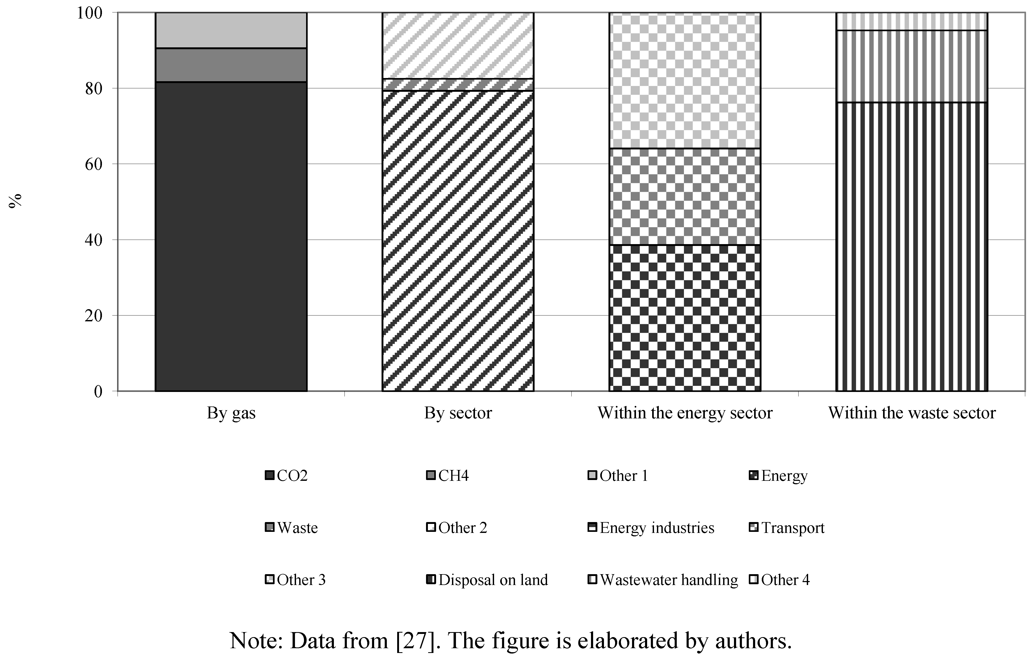
3.1. The Waste Management Sector and GHG

The classification of waste streams varies from country to country. In Lithuania, municipal solid waste (MSW) refers to household waste including similar waste from offices, small businesses, etc. [29]. According to waste records, in 2006 5700 million kg of waste was generated in Lithuania; 22.8% (1300 million kg) of which was MSW [29]. Therefore, in 2006 the per capita quantity of MSW was 390 kg, but in 2008 the waste amount increased to 407 kg [30]. Experts say that in 2010–2020 the amount of MSW should reach 1800 million kg. More than 800 landfills, which do not comply with the requirements of environment protection and public safety, were in operation until 2000. Officially, all of them were closed on the 16 of July 2009 and since then waste stream goes to 11 appropriately equipped regional landfills. However, Lithuania remains highly dependent on landfill.
Most of the waste, which now generates landfill gas (LFG), has been utilized previously and thus it is hard to believe that reliable data about its composition exists. Therefore, the article analyses only newly generated waste, i.e., it is assumed that waste composition is known. It is commonly agreed that LFG is mainly composed of 50–60% of methane and 40–50% of carbon dioxide [31,32,33,34]. Typically, carbon dioxide emission is divided into two parts: biogenic and anthropogenic emission. Assessments linked with global warming account only anthropogenic emission because biogenic carbon is considered to be “neutral”, i.e., it does not increase the net amount of CO2 in the atmosphere [35,36,37]. LFG is the product of microbiological decomposition of waste (which is primarily from biogenic sources); thus, CO2 emission from MSW is not accounted and the task is to account exclusively methane’s emission. Methane’s share within the waste sector in Lithuania is shown in Figure 2.
Figure 2. CH4 share within the waste sector in Lithuania.
Sustainability 04 01966 g002
For estimating LFG generation rates, two different approaches exist: the first approach presents LFG emission during a specific time interval, which in turn can be very different, and the second one calculates the total flux irrespective of life, i.e., until complete degradation of waste. As any urban master plan is intended for a particular period (e.g., in Lithuania it is 10 years), the question “Which is a more proper approach?” arises. When choosing the method, some general aspects must be taken into consideration: the generation of LFG does not start immediately after waste is placed in the landfill; the LFG peak is 5 to 7 years after disposal; LFG produces at a stable rate for about 20 years, but will continue to be emitted for 50 or more years. Consequently, it would be incorrect if planners simply multiplied LFG rates per year with regard to a master plan’s expiry date. The result would include only part of the threat that arises from MSW. Therefore, a more proper and fair solution is to calculate the total flux until complete degradation of waste. This approach does not offset a problem, but shows the real scale of threat and insists on finding solutions within a fixed period. The total amount of LFG varies from 100 to 200 Nm2 per 1000 kg of MSW depending on waste composition and time limit [31,34], consequential amount of CH4 (50–60%) would be 50–120 Nm2 per 1000 kg of MSW. However, a more conservative estimate of CH4 emission is about 50 Nm3 per 1000 kg of MSW [32] or 86 Nm3 per 1000 kg of MSW [31]. In general, the United States Environmental Protection Agency (USEPA) reports that CH4 emission rates can vary widely: from 6.2 to 270 Nm3 per 1000 kg of MSW and thus proposes a default value of 100 Nm3 per 1000 kg of MSW, which demonstrates a good agreement between measured and predicted emissions [38]. Lithuania does not have statistical data about an average complete quantity of methane from MSW; thus, thereinafter the applicable number is taken from abroad, i.e., 100 Nm3 per 1000 kg as proposed by USEPA. If Lithuania presents a sufficient amount of data in the future, it will be easy to change the numbers.

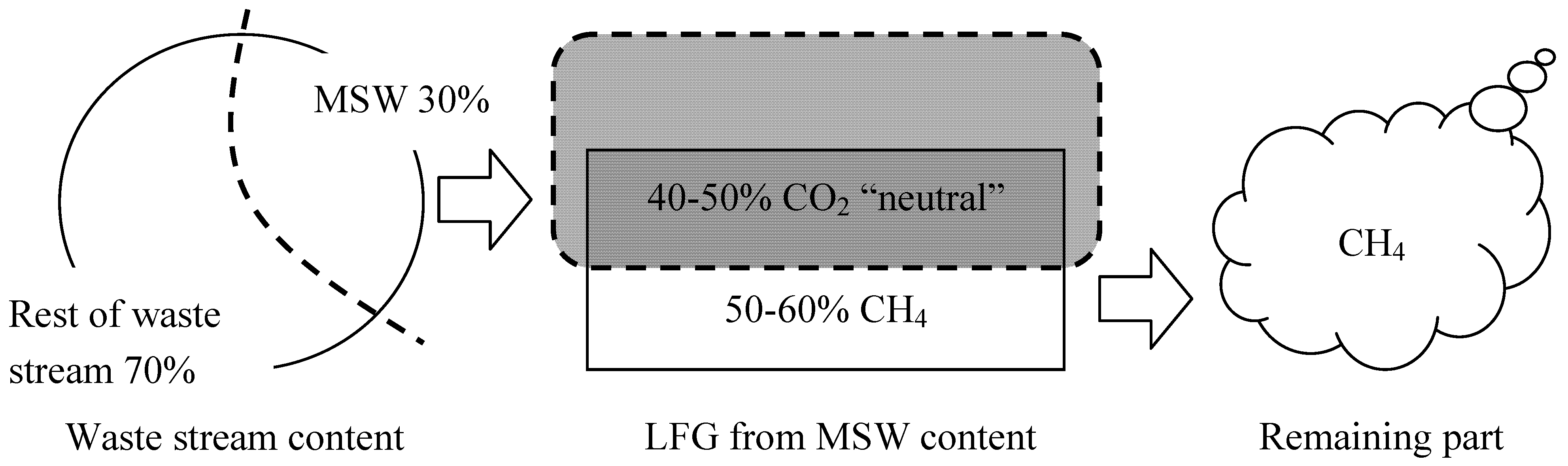
3.2. Methane Attributable to MSW
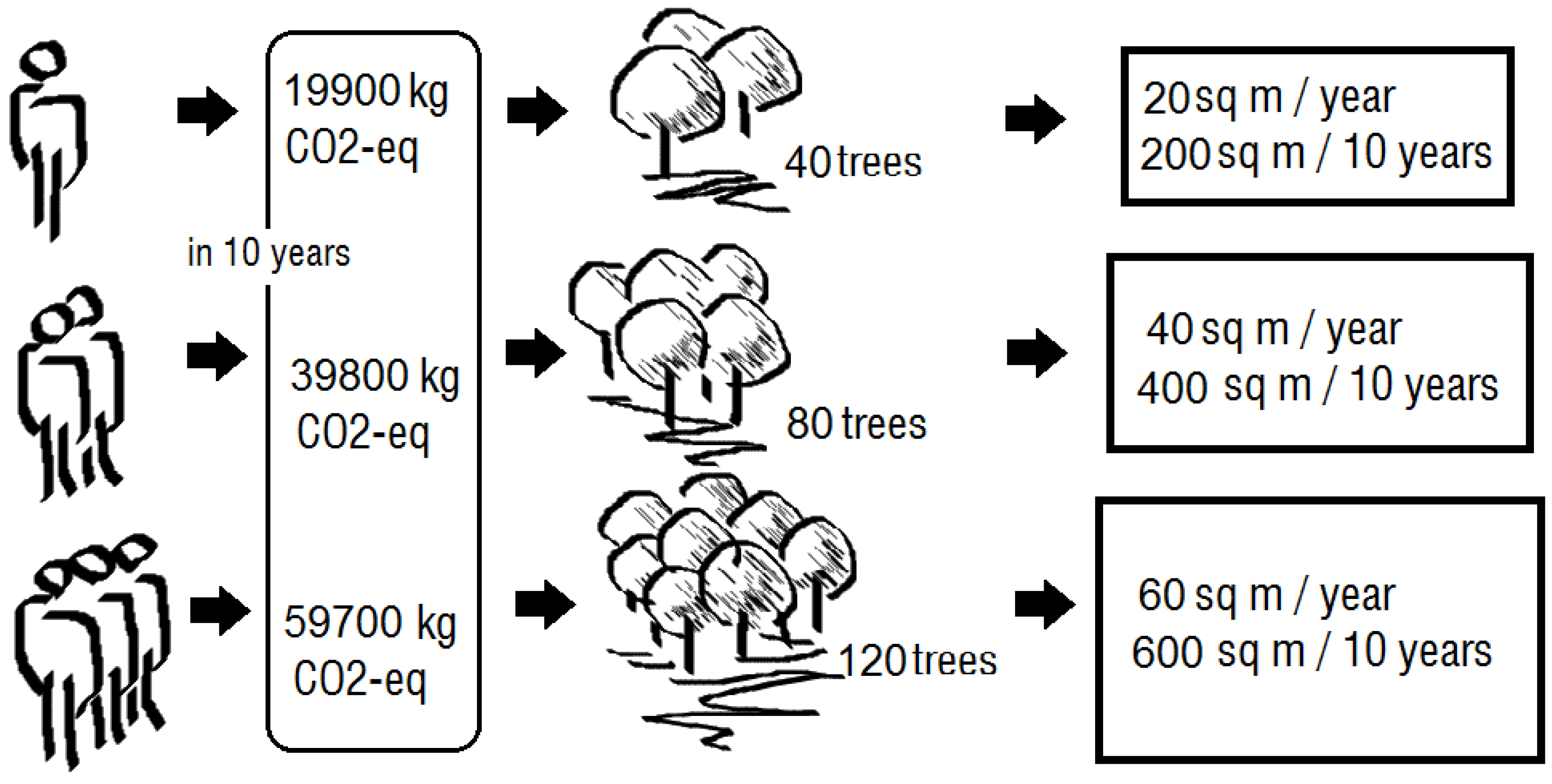
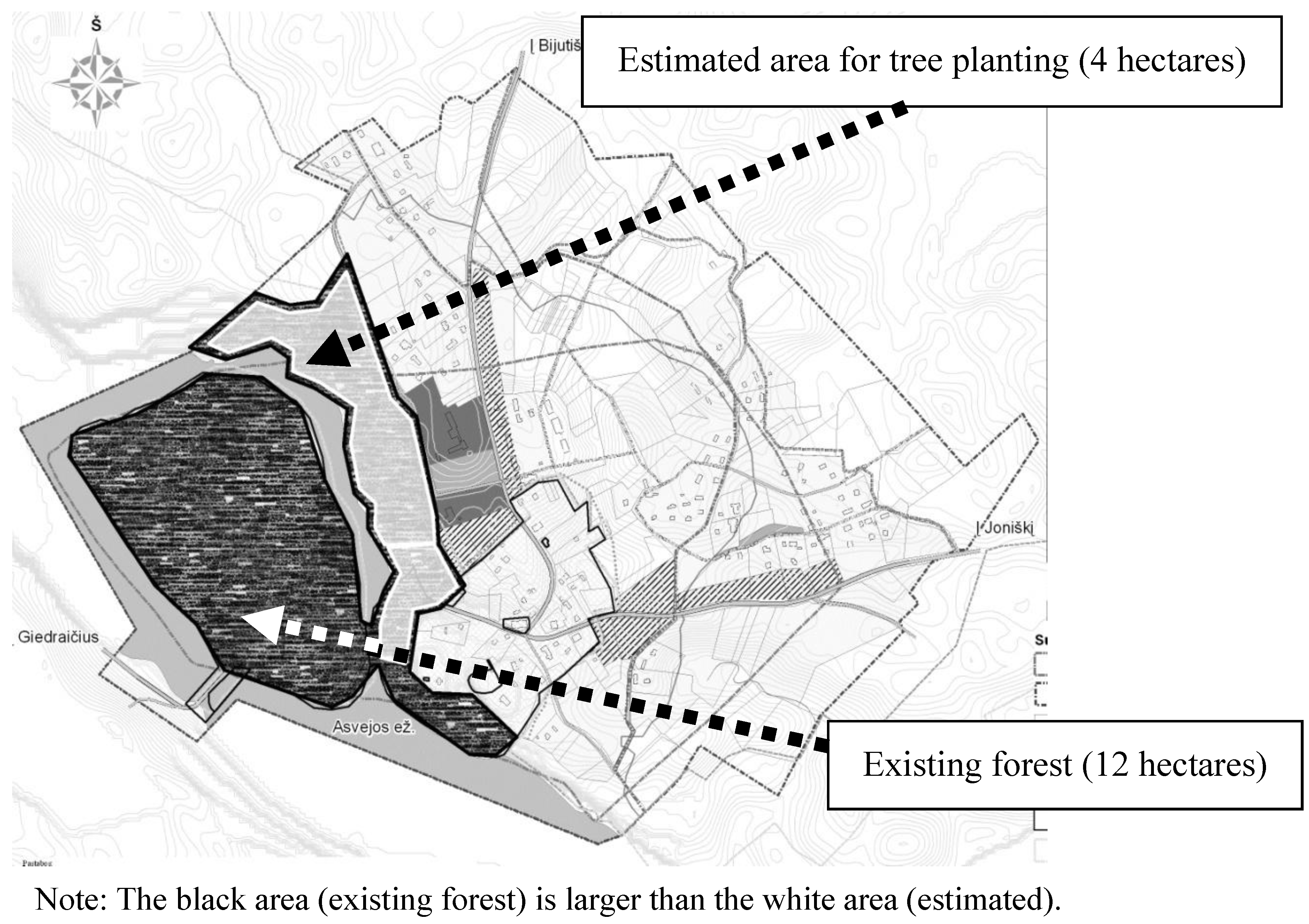
Linking urban planning with methane’s emission we can distinguish two important aspects: (1) the level of data accumulation and (2) comparability of data.
It is very important to use statistical data reported exclusively at the national level. Data on local landfill may be more precise and new, though it may differ in various cities. Therefore, there exists a threat that, for example, the city of Kaunas will use data collected since 2010 and the city of Alytus will use data compiled since 2008. This makes data incomparable and leaves room for speculation. Moreover, speaking in the context of global ecology, general information ought to be used. As it has been mentioned before, in 2008, in Lithuania per capita quantity of MSW was 407 kg [30]. It is easy to calculate the amount of generated methane (expressed in m3) until complete degradation of waste, using a simple formula (1).
Sustainability 04 01966 i001
Where M is the average methane rate (in our case 100 Nm3 per 1000 kg) and W is the total quantity of MSW per capita (in our case 407 kg). Qperson indicates that one person in a given year generates a certain amount of MSW that finally equals some cubic meters of methane.
Obviously, the amount of methane should be presented in globally comparable units. Each GHG has a different lifetime and a different ability of heat absorption; thus, gas that lasts longer and traps more heat is more damaging. An index that allows comparison is the Global Warming Potential (GWP) index—a purely physical index. GWP index is “based on the time-integrated global mean radiative forcing of a pulse emission of 1 kg of one compound relative to that of 1 kg of the reference gas CO2” [39]. Due to its readiness, GWP is broadly used in scientific as well as political areas. It is interesting to note that despite its short lifetime, methane enhances its own lifetime through changes in the OH concentration and thus its indirect effects last much longer [39]. Commonly GWP of a gas is calculated over a 100 year horizon, but other periods are also possible. Typical periods are 20 years, 100 years and 500 years. To come into contact with urban planning, a link with corresponding legislation is needed. According to Article 11 of Law on Territorial Planning, the concept of the master plan is valid for 20 years and concrete solutions are valid for 10 years [40]. The changes of GWP are not linear, thus the simple calculation of GWP of gas would be incorrect in a 10 years horizon. However, the period of 20 years is quite close and it correlates well with the expiry date of the concept of the master plan. Furthermore, GWP value in 20 years is default, so it is used very broadly. The European Common Indicators initiative‘s indicator No. 2 (local contribution to global climatic change) requires measurement in CO2 equivalent emissions (CO2-eq) [28]. Methane’s GWP in 20 years is 72; therefore, 1000 kg of methane corresponds to 72,000 kg of CO2-eq (in 20 years horizon). Equation (1) gives an answer in cubic meters, so the conversion from cubic meters to kg is needed. The Environmental Protection Agency of the United States has the Interactive Units Converter, according to it, 1 m3 of methane has a weight of 0.6802 kg [41]. For the final calculation, Equation (1) should be remodelled to Equation (2).
Sustainability 04 01966 i002
Where T is conversion coefficient, which allows recalculation of methane’s volume into weight (in our case T is 0.6802 kg), and GWPtime is methane’s GWP value of selected period. Qperson indicates that one person in a given year generates a certain amount of MSW that finally equals to some kg of CO2-eq.

4. Results

Using Equation (2), it is easy to calculate that in 2008 an average Lithuanian generated an amount of MSW that is equal to approximately 1990 kg of CO2-eq in a 20 years horizon. As this number is estimated at the national level, it can be used for preparing the master plan of any city within the territory of Lithuania. The number of citizens is easy to acquire and the proposed method is simple; therefore, it deals greatly with the idea that urban planners need aggregated information and they need it in a short period. Multiplication of 1990 by number of citizens shows a total amount of CO2-eq to be generated each year. Nevertheless, three remarks must be taken into consideration. Firstly, per capita quantity of MSW is subject to change; therefore, updates must be made constantly. The periods of measurement must be set at the national level as it guarantees comparability of data. Secondly, the quantity of waste generation is given per year and it means that the same amount is made every year. As the concrete solutions of the master plan are valid for 10 years, the final MSW amount will be 10 times bigger. However, the concept of the master plan is valid for 20 years; thus, compensation measures can be proposed within the period of 20 years. Lastly, as methane potential values are obtained from abroad (the United States), the national study of gas in local landfills would increase accurateness of the method.

5. Discussion

The ecological benefit of urban planning lies within its possibilities of mitigating the negative impact of GHG (methane in our case). The most common compensation measure linked with global warming is tree planting. One of the main reasons for this is that the Kyoto Protocol allows some remove of carbon by forests, plus planting efforts are effective, quite simple and cheap to implement. However, it is compensation in the full sense of the word, i.e., it has no effect on the decrease of MSW. If the question of the area needed for landfill was important, waste incineration would be a better and more effective solution. It is important not to mix waste incineration and the real reduction of MSW. Decrease of MSW cannot be solved in urban plan and thus is not discussed here.
Different research shows various carbon dioxide sequestration by trees e.g., between 0.5 and 2.3 kg per sq meter per year for afforestation and between 0.3 and 1.9 kg per sq meter for reforestation [42]; but it is commonly agreed that an average tree absorbs 1000 kg of carbon dioxide in its life (100 years). If tree planting is selected as compensation, a considered lifetime of a tree is very important as the sequestered amount of carbon dioxide changes due to it. Nevertheless, it is very hard to reassure that a tree will last for 100 years or that during this period it will not be cut down, or wildfire will not occur. Therefore, a 50 year life expectancy of a tree seems more adequate. To put it another way, it can be said that an average Lithuanian generates an amount of MSW per year that is equal to 1990 kg of CO2-eq in a 20 years horizon; therefore, in order to compensate this approximately 4 trees, with an expected lifetime of 50 years, are needed per year. Furthermore, during validity of the master plan solutions, the MSW amount would finally increase ten times; thus one statistical Lithuanian will produce 19,900 kg of CO2-eq, which in turn demands about 40 trees. These trees should be planted in 10 years and must survive for at least 50 years. Another possibility is tree planting in 20 years (the time of the concept), but then two master plans overlap; hence accuracy and succession are needed. Law on Plantings [43] and the acts that follow describe different specifications such as classification of plantings, accessibility, required area, etc. These acts could be easily improved with compensation mechanisms. However, the demand for planting is presented in m2 per person and therefore conversion is needed. Tree density is different according to tree species, initial spacing or intent of the planting; in Lithuania planting density varies from 1500 (asp) to 5000 (pine) trees per 10,000 sq meters [44]. Here it was assumed that the planting density is 2000 trees per 10,000 sq meters; consequently, the area of 200 m2 per person is needed to compensate 10 years CH4 emission attributable to MSW or 20 m2 each year. In brief, an assessment of MSW within urban planning and compensation mechanism is shown in Figure 3. The mechanism was tested in practice during preparation of the master plan of Dubingiai—a small town located 45 km north-east from Vilnius. The city has 215 habitants and occupies an area of 90 hectares from which 12 hectares belong to forest. Calculations revealed that roughly 4 hectares of trees were required for compensation of CO2-eq (see Figure 4); however, the forest accounted for an area three times larger than was estimated and thus additional tree planting was not necessary.
Figure 3. MSW within urban planning.
Sustainability 04 01966 g003
Figure 4. Compensation of CO2-eq in Dubingiai master plan.
Sustainability 04 01966 g004
Although tree planting is an attractive option, it remains a temporary solution: trees act as a “sink” and allow “offsets” but do not solve the problem. Moreover, 40 trees or the area of 200 m2 per person is not a concern in a small village (e.g., Dubingiai), yet it is hard or even impossible to find it in a big city. The compensation mechanism was tested in Telsiai–a city that is considerably bigger than Dubingiai (circa 20 times) and has approximately 31.6 thousand inhabitants. Calculations according to Equation 2 (or simply Figure 3) revealed that roughly 632 hectares of trees were required for compensation of CO2-eq, but currently green areas in Telsiai cover only 200 hectares, thus triple space is needed. However, in this case forests would occupy one third (sic!) of the city (see Figure 5); therefore, tree planting is feasible only in small cities and rural areas. Nevertheless, coming back to the EF and “leakage“, big cities could find supplementary areas in its districts or anywhere else in a country. In this case, accurate national statistics of planting must be made, because the possibility of overlapping or double counting exists. National data should be available to urban planners and constantly updated.
Figure 5. Compensation of CO2-eq in Telsiai master plan.
Sustainability 04 01966 g005
Waste incineration and landfill gas combustion are other options. Although incineration releases carbon dioxide, it can have a substantial advantage. Firstly, waste incineration may significantly decrease demand of landfills or the waste storage area and landfill gas burning mitigates the negative impact of otherwise uncontrolled gas leakage into the atmosphere. Secondly, under controlled conditions generated energy (captured gas) can be used for electricity or heat. Considering landfill gas burning, the efficiency for electricity production ranges between 18–26% [45] and it can reach 25–35% if landfill gas is combusted in gas engines that generate electricity and heat [31]. The efficiency for conversion of biogas into heat is even better and ranges between 40–50% [45]. However, direct combustion of MSW is a more favourable solution compared to landfill gas collection and later combustion of MSW, because it is easier to manage (control), also has more efficient energy recovery and lower carbon emissions per ton of waste (primarily due to no methane being generated) [46]. Although any waste treatment gives an ecological benefit, but credits vary depending on the type of replaced initial heat source. In 2009, in Lithuania, lion’s share of initial sources for district heating belonged to fossil fuels: 73.7% natural gas and 5,4% heating oil [47]. Thus, it is obvious that waste incineration would be a very favourable option. The major problem is that commonly heat demand is low near plants. Nevertheless, part of the generated heat can be used within the plant or distributed through district heating pipes plus this is a place where urban planners should wisely perform. The well-known Vienna’s Spittelau thermal waste treatment plant is a very successful example. It was built in order to supply a new hospital that was two kilometers away, but today Spittelay is the second largest generator in Vienna’s district heating network producing a total output of 460 MW [48]. As distance plays a major role, it must be considered at the stage of urban planning. Kollmann and Schulz state that district heating is a sensible solution but only within a radius of 5–10 km of the particular power station [49]. Furthermore, the location of the waste treatment plant within the city is ideal from the logistics point of view as it significantly reduces waste collection and delivery radius. In Lithuania there is no waste treatment plant at all; thus international successful initiatives are to be followed.

6. Conclusions

The findings of the presented research demonstrate that the EF’s practice of environmental limits and the “leakage” effect could be transferred into urban planning. Furthermore, the European Common Indicators Initiative proposes 10 indicators reflecting actions towards sustainability; three of these indicators are strongly bound up with urban ecology. If the indicator concerning MSW was merged with the EF’s practice, then the negative impact of MSW could be prevented (or at least mitigated) at the stage of urban planning. Taking Lithuania as an example (here the situation concerning MSW treatment is very similar to other post-soviet countries), it has been estimated that an average Lithuanian in 10 years generates an amount of MSW, which is equal to 19,900 kg of CO2-eq in a 20 years horizon. Therefore, compensation of the gases requires roughly 40 trees which is equal to 200 m2 in turn. Although such a method would be feasible only in extended cities, big cities could rely on the “leakage” practice. Lastly, if urban planning involves waste incineration, heat generation would be a sensible solution. However, heat plants should supply heat within a radius of 5–10 km of the power station.

Acknowledgements

The authors are in debt to David Morley for proofreading of the manuscript.

Conflict of Interest

The authors declare no conflict of interest.

References

  1. Millennium Ecosystem Assessment, Ecosystems and Human Well-Being: Synthesis; General Synthesis; Island Press: Washington, DC, USA, 2005.
  2. Singh, R.K.; Murty, H.R.; Gupta, S.K.; Dikshit, A.K. An overview of sustainability assessment methodologies. Ecol. Indic. 2009, 9, 189–212. [Google Scholar]
  3. Böhringer, C.; Jochem, P.E.P. Measuring the immeasurable—A survey of sustainability indices. Ecol. Econ. 2007, 63, 1–8. [Google Scholar]
  4. Wackernagel, M.; Moran, D.; Goldfinger, S.; Monfreda, C.; Welch, A.; Murray, M.; Burns, S.; Königel, C.; Peck, J.; King, P.; et al. Europe 2005: The Ecological Footprint; Report; WWF European Policy Office: Brussels, Belgium, 2005. [Google Scholar]
  5. Eurostat. Urban rankings 2011-Statistics Explained. Available online: http://epp.eurostat.ec.europa.eu/statistics_explained/index.php/Urban_rankings (accessed on 11 January 2011).
  6. Environment Terminology and Discovery Service, European Environment Agency. Available online: http://glossary.eea.europa.eu/terminology/concept_html?term=ecology (accessed on 5 December 2010).
  7. Ewers, R.M.; Smith, R.J. Choice of index determines the relationship between corruption and environmental sustainability. Ecol. Soc. 2007, 12, 1–6. [Google Scholar]
  8. Mayer, A.L. Strengths and weaknesses of common sustainability indices for multidimensional systems. Environ. Int. 2008, 34, 277–291. [Google Scholar] [CrossRef]
  9. Siche, J.R.; Agostinho, F.; Ortega, E.; Romeiro, A. Sustainability of nations by indices: Comparative study between environmental sustainability index, ecological footprint and the emergy performance indices. Ecol. Econ. 2008, 66, 628–637. [Google Scholar] [CrossRef]
  10. Monfreda, C.; Wackernagel, M.; Deumling, D. Establishing national natural capital accounts based on detailed ecological footprint and biological capacity assessments. Land Use Pol. 2004, 21, 231–246. [Google Scholar] [CrossRef]
  11. Kitzes, J.; Galli, A.; Bagliani, M.; Barrett, J.; Dige, G.; Ede, S.; Erb, K.; Giljum, S.; Haberl, H.; Hails, C.; et al. A research agenda for improving national Ecological Footprint accounts. Ecol. Econ. 2009, 68, 1991–2007. [Google Scholar] [CrossRef]
  12. Esty, D.C.; Levy, M.; Srebotnjak, T.; de Sherbinin, A. 2005 Environmental Sustainability Index: Benchmarking National Environmental Stewardship; Main report; Yale Center for Environmental Law & Policy: New Haven, CT, USA, 2005. [Google Scholar]
  13. Esty, D.C.; Levy, M.; Srebotnjak, T.; de Sherbinin, A. 2005 Environmental Sustainability Index: Benchmarking National Environmental Stewardship—Appendix A. Methodology; Yale Center for Environmental Law & Policy: New Haven, CT, USA, 2005. [Google Scholar]
  14. Hails, C.; Humphrey, S.; Loh, J.; Goldfinger, S. Living Planet Report 2008; World Wide Fund For Nature: Gland, Switzerland, 2008. [Google Scholar]
  15. Morse, S.; Fraser, E.D.G. Making “dirty” nations look cleans? The nation state and the problem of selecting and weighting indices as tools for measuring progress towards sustainability. Geoforum 2005, 36, 625–640. [Google Scholar] [CrossRef]
  16. Strange, T.; Bayley, A. Sustainable Development: Linking Economy, Society, Environment; OECD Publications: Paris, France, 2008; pp. 20–35. [Google Scholar]
  17. Esty, D.C.; Levy, M.; Srebotnjak, T.; de Sherbinin, A. 2005 Environmental Sustainability Index: Benchmarking National Environmental Stewardship—Appendix H. Critiques and Responses; Yale Center for Environmental Law & Policy: New Haven, CT, USA, 2005. [Google Scholar]
  18. Ong, B.L. Green plot ratio: An ecological measure for architecture and urban planning. Landsc. Urban Plan. 2002, 63, 197–211. [Google Scholar] [CrossRef]
  19. Fiala, N. Measuring sustainability: Why the ecological footprint is bad economics and bad environmental science. Ecol. Econ. 2008, 67, 519–525. [Google Scholar] [CrossRef]
  20. Venetoulis, J.; Talberth, J. Refining the ecological footprint. Environ. Dev. Sustain. 2008, 10, 441–469. [Google Scholar] [CrossRef]
  21. Pickett, S.T.A.; Cadenasso, M.L.; Grove, J.M.; Boone, C.G.; Groffman, P.M.; Irwin, E.; Kaushal, S.S.; Marshall, V.; McGrath, B.P.; Nilon, C.H.; et al. Urban ecological systems: Scientific foundations and a decade of progress. J. Environ. Manag. 2011, 92, 331–362. [Google Scholar]
  22. Groc, I. Keep your footprint out of my backyard. Planning 2007, 73, 32–35. [Google Scholar]
  23. White, T.J. Sharing resources: The global distribution of the Ecological Footprint. Ecol. Econ. 2007, 64, 402–410. [Google Scholar] [CrossRef]
  24. Global Footprint Network. Trends-Kuwait. Available online: http://www.footprintnetwork.org/ en/index.php/GFN/page/trends/kuwait/ (accessed on 15 December 2010).
  25. Tarzia, V. European Common Indicators: Towards a Local Sustainability Profile; Final Project Report; Ambiente Italia Research Institute: Milano, Italy, 2003. [Google Scholar]
  26. Urban Environment, European Commission. Available online: http://ec.europa.eu/environment/ urban/common_indicators.htm (accessed on 5 December 2010).
  27. UNFCCC. Summary of GHG Emissions for European Union. Available online: http://unfccc.int/files/ghg_data/ghg_data_unfccc/ghg_profiles/application/pdf/eu-27_ghg_profile.pdf (accessed on 8 February 2012).
  28. Urban Environment, European Commission. Towards a Local Sustainability Profile-European Common Indicators-Methodology sheets. Available online: http://ec.europa.eu/environment/ urban/pdf/methodology_sheet_en.pdf (accessed on 5 December 2010).
  29. Government of the Republic of Lithuania. National Strategic Waste Management Plan. Available online: http://www3.lrs.lt/pls/inter3/dokpaieska.showdoc_l?p_id=344021&p_query=&p_tr2= (accessed on 12 May 2010).
  30. Eurostat. Waste Statistics 2011-Statistics Explained. Available online: http://epp.eurostat.ec.europa.eu/statistics_explained/index.php/Waste_statistics (accessed on 11 January 2011).
  31. Manfredi, S. Environmental Assessment of Solid Waste Landfilling in a Life Cycle Perspective (LCA Model EASEWASTE). Ph.D. Thesis; Technical University of Denmark, June 2009. Available online: http://www2.er.dtu.dk/publications/fulltext/2009/ENV2009-145.pdf (accessed on 16 December 2010).
  32. Themelis, N.J.; Ulloa, P.A. Methane generation in landfills. Renew. Energ. 2007, 32, 1243–1257. [Google Scholar] [CrossRef]
  33. U.S. Environmental Protection Agency. Facts About Landfill Gas. Available online: http://www.dem.ri.gov/programs/benviron/waste/central/lfgfact.pdf (accessed on 27 November 2010).
  34. Verma, S. Anaerobic Digestion of Biodegradable Organics in Municipal Solid Wastes, 2002. Columbia University Earth Engineering Center for Sustainable Waste Management. 2002. Available online: http://www.seas.columbia.edu/earth/vermathesis.pdf (accessed on 10 January 2011).
  35. U.S. Environmental Protection Agency, Climate Leaders Greenhouse Gas Inventory Protocol —Offset Project Methodology —For Project Type: Reforestation/Afforestation; U.S. EPA: Washington, DC, USA, 2008.
  36. Gentil, E.; Christensen, T.H.; Aoustin, E. Greenhouse gas accounting and waste management. Waste Manag. Res. 2009, 27, 696–706. [Google Scholar] [CrossRef]
  37. Scheutz, C.; Kjeldsen, P.; Gentil, E. Greenhouse gases, radiative forcing, global warming potential and waste management—An introduction. Waste Manag. Res. 2009, 27, 716–723. [Google Scholar] [CrossRef]
  38. U.S. Environmental Protection Agency, Background Information Document for Updaring AP42 Section 2.4 for Estimating Emissions from Municipal Solid Waste Landfills; EPA/600/R-08-116; U.S. EPA: Washington, DC, USA, September 2008; (accessed on 10 July 2012). Available online: http://www.epa.gov/ttn/chief/ap42/ch02/draft/db02s04.pdf.
  39. Forster, P.; Ramaswamy, V.; Artaxo, P.; Berntsen, T.; Betts, R.; Fahey, D.W.; Haywood, J.; Lean, J.; Lowe, D.C.; Myhre, G.; et al. Contribution of Working Group I to the Fourth Assessment Report of the Intergovernmental Panel on Climate Change. In Changes in Atmospheric Constituents and in Radiative Forcing; Cambridge University Press: Cambridge, UK, 2007. [Google Scholar]
  40. Seimas of the Republic of Lithuania. Law on Territorial Planning. Available online: http://www3.lrs.lt/pls/inter2/dokpaieska.showdoc_l?p_id=378358 (accessed on 24 September 2010).
  41. U.S. Environmental Protection Agency. Interactive Units Converter Coalbed Methane Outreach Program (CMOP). Available online: http://www.epa.gov/cmop/resources/converter.html (accessed on 7 December 2010).
  42. Gorte, R.W. U.S. Tree Planting for Carbon Sequestration; CRS Report for Congress R40562; Congressional Research Service: Washington, DC, USA, 2009. [Google Scholar]
  43. Seimas of the Republic of Lithuania. Law on Plantings. Available online: http://www3.lrs.lt/pls/inter3/dokpaieska.showdoc_l?p_id=386835 (accessed on 12 December 2010).
  44. Seimas of the Republic of Lithuania. Reforestation and Afforestation Policies. Available online: http://www3.lrs.lt/pls/inter3/dokpaieska.showdoc_l?p_id=318353&p_query=&p_tr2= (accessed on 4 January 2011).
  45. Fruergaard, T.; Astrup, T.; Ekvall, T. Energy use and recovery in waste management and implications for accounting of greenhouse gases and global warming contributions. Waste Manag. Res. 2009, 27, 724–737. [Google Scholar]
  46. Kaplan, P.O.; DeCarolis, J.; Thorneloe, S. Is it better to burn or bury waste for clean electricity generation? Environ. Sci. Technol. 2009, 43, 1711–1717. [Google Scholar]
  47. Lithuanian District Heating Association. Economic Activity Review of Heat Supply Companies in 2009. Available online: http://www.lsta.lt/files/statistika/2009_apzvalga.pdf (accessed on 10 January 2011).
  48. Wien Energie Spittelau. The thermal waste treatment plant. Available online: http://www.wienenergie.at/media/files/2008/technik-bro-spittelau%20-%20englisch_9396.pdf (accessed on 10 January 2011).
  49. Richarz, C.; Schulz, C.; Zeitler, F. Upgrading the Installations. Heating Installation. In Energy–Efficiency Upgrades, 1st; Kollmann, N., Schulz, C., Eds.; Birkhäuser: Basel, Switzerland, 2007; pp. 58–63. [Google Scholar]

