Asymptotic Behavior of a Delay Differential Neoclassical Growth Model

Abstract

A neoclassical growth model is examined with a special mound-shaped production function. Continuous time scales are assumed and a complete steady state and stability analysis is presented. Fixed delay is then assumed and it is shown how the asymptotic stability of the steady state is lost if the delay reaches a certain threshold, where Hopf bifurcation occurs. In the case of continuously distriubuted delays, we show that with small average delays stability is preserved, then lost at a threshold, then it is regained if the average delay becomes sufficiently large. The occurence of Hopf bifurcation is shown at both critical values.

1. Introduction

The examination of economic growth models is one of the most frequently discussed issues in mathematical economics. Day [1,2] has investigated a neoclassical growth model, and a productivity and population growth model and showed the emergence of complex behavior even under simple economic structure. His models were based on discrete time scales and a mound-shaped production function that represented the negative effect of pollution resulting from increasing capital. It was demonstrated by numerical computations that these models could generate cyclic and even chaotic behavior. Following Day’s pioneering works, a lot of effort has been given to the understanding of complex economic dynamics. Day [3], Puu [4] and Bischi et al. [5] present the earlier contributions of this field. A large number of studies assumed discrete time scales. Li and Yorke [6] have introduced the “period-three condition” to detect chaos, which has many applications in first-order nonlinear difference equations. The papers collected by Rosser [7] offer many applications. Only a few studies are devoted to the case of continuous time scales, since there is no general criterion to detect chaos and the system must have at least three dimensions.

In this paper, we will examine an extension of the neoclassical growth model, which can be traced back to the early works of Solow [8] and Swan [9]. The neoclassical growth model is constructed with the two (usually implicitly mentioned) assumptions; one is the full-employment of labor and capital and the other is instantaneous adjustment in the output market. Thus, it is suitable for describing the long-run behavior of the economy. Due to the well-behaved production function, the steady state of the model is usually asymptotically stable. However, it is often observed in reality that growth path exhibits persistent fluctuations. The neoclassical model could be the good point of departure to show how such persistent behavior can emerge when nonlinearities and a production lag are present. Matsumoto and Szidarovszky [10] attempt to fill the gap and have introduced a neoclassical model with a mound-shaped production function that was assumed to be a Cobb-Douglas type function of the form F(x)=Ax^a(1 - x)^b with x being the capital per unit labor. Although they show emergence of erratic fluctuations in the capital accumulation process, the production function is restrictive in the sense that it is defined only in the unit interval. This paper modifies this drawback, considers another type of mound-shaped production function and will examine the stability of the steady state with and without time delays in the continuous-time framework. Two kinds of delays will be discussed, fixed and continuously distributed (continuously hereafter) delays. We keep the relatively simple model of Matsumoto and Szidarovszky [10] in order to be able to compare the results and to illustrate that complex dynamics can be generated under simple economic assumptions with both function types.

This paper develops as follows. First the mathematical model is formulated without time delays, and complete steady state and stability analysis is presented. Then, models with fixed delays and then with continuous delays are introduced and complete stability analysis is given. The last section concludes the paper.

2. The Mathematical Model

Matsumoto and Szidarovszky [10] have introduced a special growth model of the form

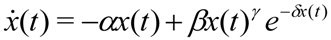
where x is the capital per labor, s and α are positive parameters where s ∈ (0,1) is the average propensity to save and α = n+sμ with μ being the depreciation ratio of capital and n the growth rate of labor. In applying the Cobb-Douglas type function F(x) = Ax^α (1 - x)^b the value of x has to be normalized into the (0,1) interval. In this paper we will assume that

F(x) = εx^γe^-δx,

which is a mound-shaped function in which x can take any positive value. This function has zero value at x = 0, converges to zero as x → ∞, increases for x < γ / δ and decreases for x > γ / δ， so it has its maximum at x = γ / δ. The drawbacks of the neoclassical production function that ignores natural resource or energy are partly remedied in our function. δ of the exponential term reflecting a strength of a “negative effect” caused by increasing concentration of capital. The value of δ is exogenously given, however, can be thought to be determined by a damaging degree of natural environment or energy resources. With the modified function, the mathematical model becomes

(1)

where α, γ, δ and β = s ε are positive parameters. The number of steady states and their locations depend on the specific values of the model parameters. We will consider three different cases: γ < 1, γ = 1 and γ > 1. We can give the following interpretation for the value of the parameter γ of the production function; γ can be thought as a proxy for measuring returns to scale of the production function. Indeed, when x is small (i.e., the exponential term is close to unity), output increases more than unity, exactly unity and less than unity if γ > 1, γ = 1 and γ < 1, respectively. Let now f(x) denote the right hand side of equation (1). If x(0) = 0, then the identically zero function is a solution which case is not interesting from the economic point of view and is eliminated from further considerations

Case I.

Assume first that γ < 1. The steady states are the solutions of f(x) = 0. Notice that f(0) = 0, so zero is a steady state. f(x) converges to - ∞ as x → ∞ Since

f´(x) = -α + βγx^γ-1e^-δx- βδx^γe^-δx

f´(x) converges to ∞ as x tends to zero with positive values. Hence f(x) increases for small values of x > 0. The steady state equation f(x) = 0 can be written as

x^γ (-αx^1-γ + βe^-δx) = 0

(2)

so the positive steady state is the unique solution of equation

αx^1-γ = βe^-δx

(3)

The left hand side is zero at x = 0 and strictly increasing, furthermore, converges to ∞ as x tends to infinity. The right hand side is β > 0 at x = 0, strictly decreases and converges to zero as x → ∞. Hence there is a unique solution > 0 of (3), and f(x) > 0 if x < and f(x) < 0 as x > These relations imply that if x(0) < , then x (t) increases and converges to , and if x (0) > , then x (t) decreases and converges to . If x(0) = , then x (t) remains for all x > 0. Thus is globally asymptotically stable.

Case II.

Assume next that γ = 1. Then the steady state equation has the form

x(-α + βe^-δx) = 0

(4)

so zero is a steady state and there is a unique root of the second factor,

(5)

If β ≤ α, then the value of f(x) is negative for all x > 0. Therefore x(t) is decreasing and converges to zero with arbitrary x (0) > 0. If β > α, then > 0, furthermore f(x) > 0 as x < , and f(x) < 0 as x > . If x (0) < , then x (t) increases and if x (0) > , then x decreases and converges to , and if x (0) = , then x (t) remains for all T > 0 Hence is globally asymptotically stable.

Case III.

Consider finally the case of γ > 1. The steady state equation has now the form

x(-α + βx^γ-1e^-δx) = 0

(6)

so zero is a steady state again, and any other steady state is the solution of equation

g(x) = -α + βx^γ-1e^-δx = 0

(7)

Notice that

and

g´(x) = β(γ-1)x^γ-2e^-δx - βδx^γ-1e^-δx

= βx^γ-2e^-δx(γ-1 - δx)

Therefore g(x) as its global maximum at

(8)

increases for x < and decreases for x > . Now we have three sub-cases.

(i) if g( ) < 0, then there is no positive steady state and with arbitrary x(0)>0, x(t) decreases and converges to zero.

(ii) if g( ) < 0, then = is the unique positive steady state and f(x) < 0 for all 0 < x ≠ . If x(0) < , then x (t) decreases and converges to 0, and if x(0) > then x (t) decreases again and now converges to . If x(0) = , then x (t) = for all t > 0.

(iii) If g( ) > 0, then equation (7) has two positive solutions, ₁ < and ₂ > . Relation (6) implies that f(x) < 0 as x < ₁ or x > ₂, and f(x) > 0 if ₁ < x < ₂. Therefore if x(0) < ₁, then x (t) decreases and converges to zero, if ₁ < x(0) < ₂, then x (t) increases and converges to ₂, if x (0) > ₂, then x (t) decreases and converges to ₂. That is, ₁ is locally unstable and ₂ is locally asymptotically stable. If x(0) = ₁ or x (0) = ₂, then x (t) remains at that steady state level for all t > 0.

3. Model with Fixed Delay

The fixed delay T > 0 is assumed in the second term of the right hand side of equation (1), so we have the following equation:

(9)

Where

h(x) = βx^γe^-δx

(10)

The local asymptotic behavior of the trajectory can be examined by linearization. Let be a positive steady state. Then the linearized equation has the form

where x_δ(t) is the deviation of x (t) from the steady state level. Looking for the solution in the usual form x_δ(t) = e^λtu, we have

which gives the characteristic equation

or

(11)

Lemma 1 Assume that |h´( )| < α. Then is locally asymptotically stable.

Proof. Assume that Re λ ≥ 0. Then

|λ + α| ≥ α

and since

e^λT = e^T(Reλ)e^iT(Imλ)

= e^T(Reλ)(cos[T(Imλ)] + isin[T(Imλ)])

clearly

|e^λT| ≥ 1

Therefore

implying that λ cannot be an eigenvalue. Q.E.D.

Notice that

h´(x) = βx^γ-1e^-δx(γ - δx)

(12)

and at the steady state

βx^γe^-δx = αx

implying that

βx^γ-1e^-δx = α

Therefore

(13)

so the characteristic equation (11) can be rewritten as

We also mention that the condition of Lemma 1 can be rewritten as

or equivalently

(14)

In the special case of γ = 1, this condition has the form

which is equivalent to relation

α < β < αe²

In order to give a complete stability analysis, we have to find the possible stability switches. Substituting any stability switch, λ= iω with ω > 0 into equation (11) yields

(15)

Separating the real and imaginary parts gives two equations,

(16)

and

(17)

Adding the squares of these equations gives

so

(18)

In order to have solution we have to assume now that

(19)

that is, (14) is violated with strict inequalities. Concerning this assumption, we can give the following interpretation. Let F(x) be y. Then

So this means that the absolute value of the elasticity of output with respect to capital is larger than unity. From (16) we have that if h΄( )>0, then T⁽ⁿ⁾ = T₊⁽ⁿ⁾ with

(20)

and if if h´( ) < 0, then T ⁽ⁿ⁾ = T_-⁽ⁿ⁾ with

(21)

and by (13) and (19),

so h´( ) cannot be zero.

By selecting T as the bifurcation parameter and implicitly differentiating the characteristic equation with respect to T, we have

implying that

If λ = iω, then

with real part

Therefore if a steady state is unstable with T = 0, then it remains unstable for all T > 0, and if a steady state is asymptotically stable at T = 0, then this stability is lost at T = T⁽⁰⁾ and cannot be regained later. That is, if the steady state is unstable without delay, then it remains unstable with any delay of positive length. If the steady state is asymptotically stable without delay, then it remains asymptotically stable until the delay reaches a certain threshold, and then becomes unstable and the stability cannot be regained later.

Taking, α = 1, β = 25, γ = 1 and δ = 1, we give an illustrative numerical example in Figure 1. The critical value γ - δ is denoted by

Introducing the notation z = γ - δ transforms the T _-⁽⁰⁾ curve to

and then the corresponding critical value of the delay is

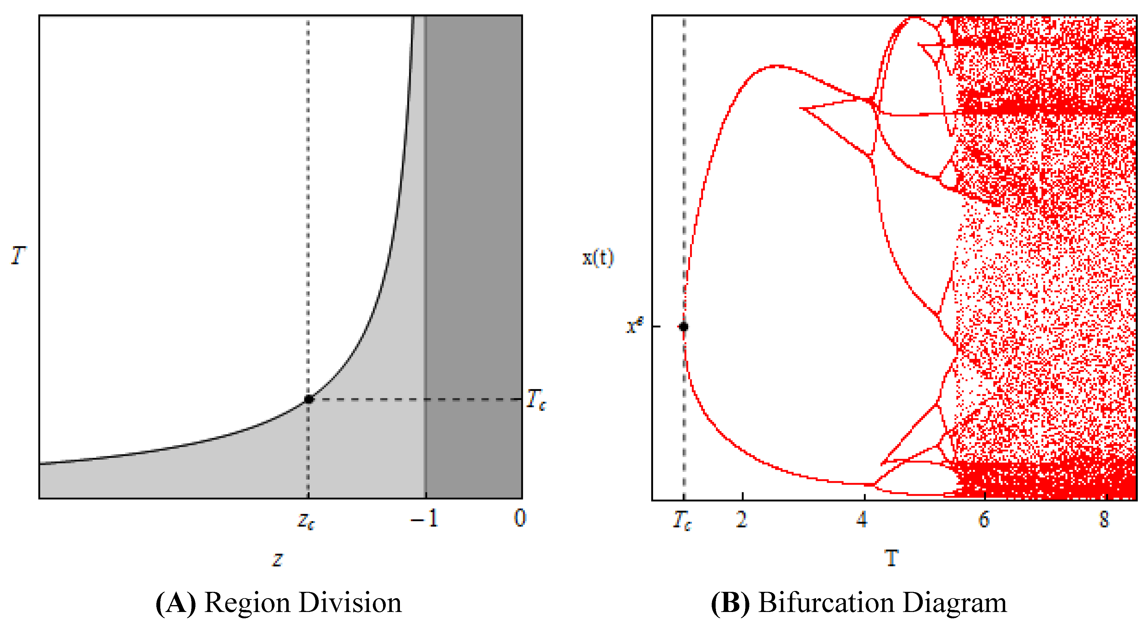
In Figure 1(A), the steady state is locally asymptotically stable in the dark-gray region with z > -1 due to Lemma 1. It is also locally asymptotically stable in the light-gray region, which is under the critical curve T = T_-⁽⁰⁾ and it is unstable in the white region above the curve. Setting z = z_c and increasing T along the vertical dotted line in Figure 1(A), we can see that the steady state loses stability at T = T_c. Further increasing T , as observed in Figure 1(B), generates complex dynamics through a quasi period-doubling bifurcation in which T increases from T _c- 0.05 to 8.5 with an increment of 0.01 and the local maximum and minimum of the corresponding trajectory are plotted against each value of T.

Figure 1. Dynamics with α = 1, β = 25, γ = 1 and δ = 1.

Figure 1. Dynamics with α = 1, β = 25, γ = 1 and δ = 1.

4. Model with Continuously Distributed Delay

Assuming continuously distributed delays in the second term of equation (1) gives the following Volterra-type integro-differential equation:

(22)

where T > 0 is a positive parameter, the average delay and m ≥ 0 is an integer. The kernel function has the form

If m = 0, then the most current value has the highest weight, which is then decreasing exponentially. If m ≥ 1, then the most current value has zero weight which is then increasing until t - s = T, and is decreasing exponentially afterwards. As m increases, the weighting function becomes more peaked around t - s = T and as m → ∞, it converges to the Dirac delta function centered at t - s = T. If T → 0, then it also converges to the Dirac delta function.

A similar model is investigated by Fanti and Manfredi [11] where m = 2 is selected and the stability of the system with a cubic characteristic polynomial is examined based on the Routh-Hurwitz criterion. Stamova and Stamov [12] consider a generalized Solow model with endegenous labor growth and impulsive perturbations. Their stability analysis is based on the Lyapunov-Razumikhin sufficient stability conditions, which is a different approach than ours.

Linearizing equation (22), we have

where x_δ(t) is the deviation of x (t) from the steady state level . We are looking for the solution in the usual exponential form

x_δ(t) = e^λtu

then simple substitution shows that

Notice that by introducing the length of the delay as the new variable S = t - s in the integral, we see that

and by letting T → ∞, we have the characteristic equation

with

This equation can be rewritten as

(23)

Then similarly to the case of fixed delay we can prove the following result:

Lemma 2 Assume that |h´( )| < α. Then is locally asymptotically stable.

Proof. Assume that Reλ≥ 0. Then

therefore

implying that λ cannot be a solution of equation (23). Q.E.D.

It is well known that the Routh-Hurwitz stability theorem provides necessary and sufficient conditions for all roots of a polynomial equation with real coefficients to have negative real parts. It is also known that it is difficult to locate the eigenvalues with analytic methods in general. However in some special cases, analytic results are still possible to obtain, as it will be next demonstrated.

Case I. T = 0

Assume first that T = 0, which reduces equation (22) with delays to equation (1) without delays. The asymptotic properties of this equation were already discussed earlier.

Case II. T > 0 and m = 0

Assume next that T > 0 and m = 0, when the kernel function becomes exponentially declining. Then characteristic equation (23) becomes quadratic,

or

(24)

If γ ≤ 1, then all coefficients are positive with a positive steady state, which is locally asymptotically stable. Assume next that γ > 1. If

then the constant term is zero indicating that one eigenvalue is zero and the other is negative. So is marginally stable in the linearized model, so no conclusion can be drawn about its asymptotical behavior in the nonlinear model. If < (γ - 1)/δ, then is unstable and if > (γ - 1)/δ, then is locally asymptotically stable.

Case III. T > 0 and m = 1

Assume now that T > 0 and m = 1, when the shape of the kernel function takes a bell-shaped form. Then we have a cubic characteristic polynomial:

or

(25)

If γ ≤ 1, then all coefficients are positive at a positive steady state. If γ > 1, then we can consider three cases. If

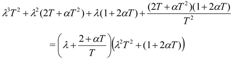
then zero is an eigenvalue and the other two eigenvalues have negative real parts implying that in the linearized system is marginally stable. Therefore no conclusion can be drawn about the stability of in the nonlinear system. If < (γ - 1)/δ, then the constant term is negative, so is unstable. If > (γ - 1)/δ then all coefficient of (25) are positive. In this case and when γ ≤ 1 the Routh-Hurwitz criterion implies that the real parts of the eigenvalues are negative if and only if

which can be reduced to a quadratic inequality in T:

(26)

For the sake of simplicity, we re-introduce the notation = γ - δ . If z ≥ 0, then this inequality holds implying the asymptotical stability of the steady state.So we can assume that z < 0.The discriminant of the left hand side of inequality (26) is

D = z(z + 8)

If z < -8, then D > 0, so the left hand side of (26) has two roots

(27)

which are positive and < . Notice that = 1/α² and (26) holds if and only if T < or T > when is locally asymptotically stable. If < T < , then (26) is violated, so is unstable. If z = -8, then D = 0 and there are equal roots

so if T ≠ 1/α, then is locally asymptotically stable.

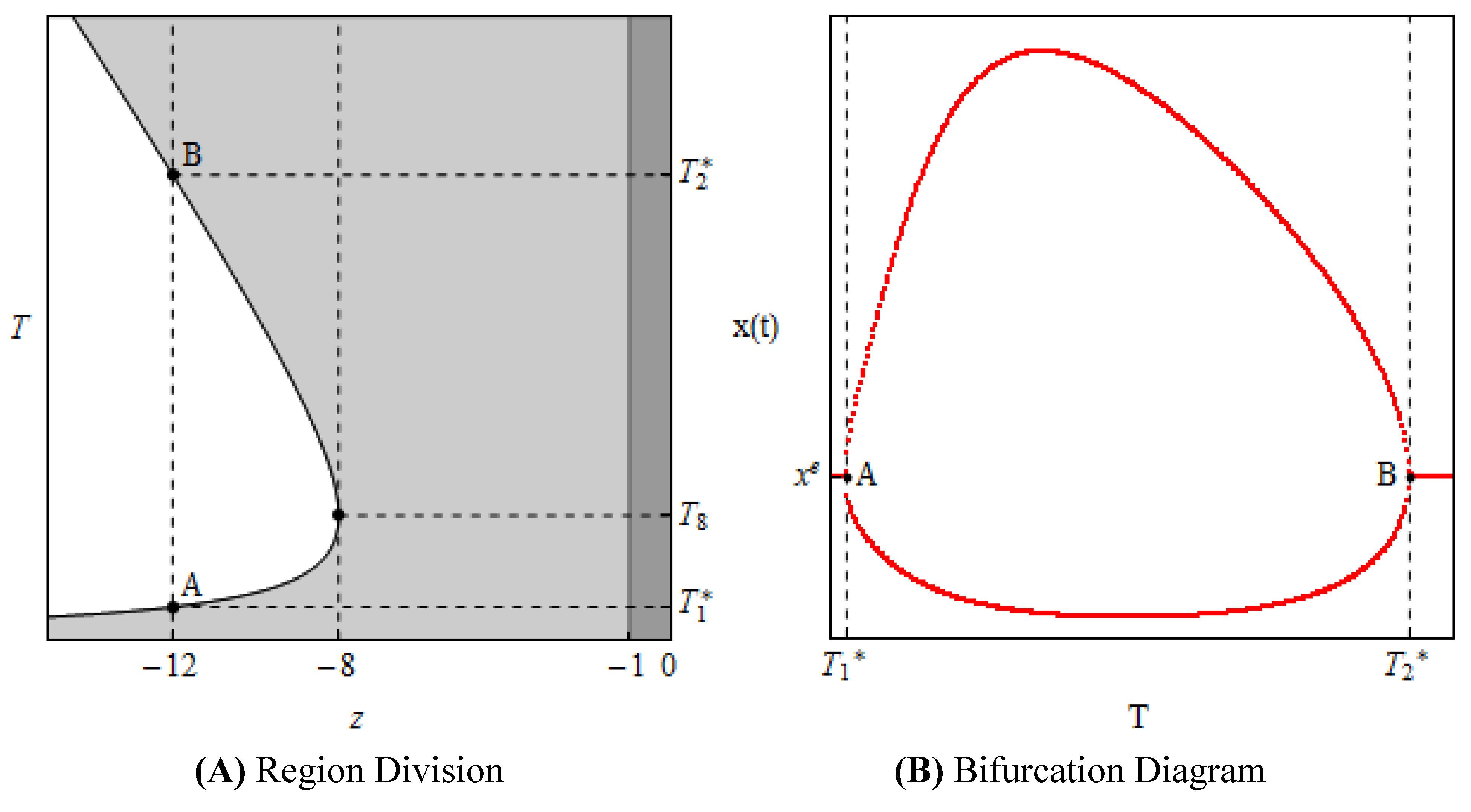
If -8 < z < 0, then D < 0, so (26) holds and is asymptotically stable. The instability region is shown in Figure 2(A) where z is the horizontal axis and T is the vertical axis. If we start with a very small value of T with any given z < -8, then is asymptotically stable. If we gradually increase T then remains asymptotically stable until it reaches the critical value , when the steady state becomes unstable. It remains unstable until when stability is regained, and remains asymptotically stable for all T > .

If the steady state is unstable without delay, then it remains unstable with continuous delay with any T and m. If it is asymptotically stable without delay, then either it remains asymptotically stable with all T and m, or loses stability at a certain value of the average delay T and stability is regained with an even larger value of T and the steady state remains asymptotically stable afterwards. In such cases small and large average delays lead to asymptotically stable steady states.

We will next show that at the critical values and , Hopf bifurcation occurs giving the possibility of the birth of limit cycles. We select T as the bifurcation parameter. At the critical values (26) is satisfied with equality, so

and the characteristic equation (25) can be rewritten as

showing that there is a negative eigenvalue

and a pair of pure complex eigenvalues

Consider λ as a function of the bifurcation parameter T and differentiate implicitly equation (25) to have

By simple calculation we can see that at λ = ± iε,

with real part

Since = 1/α², at T = the value of d(Reλ)/dT changes from negative to positive showing the loss of stability, and if T = , then d(Reλ)/dT changes from positive to negative indicating that stability is regained. Since at both critical values d(Reλ)/dT ≠ 0, at both values Hopf bifurcation occurs giving the possibility of the birth of limit cycles.

We perform numerical simulations to illustrate the results obtained above. In Figure 2(A), the steady state is locally asymptotically stable in the dark-gray region with z > -1 due to Lemma 2. It is also locally asymptotically stable in the light gray region and unstable in the white region when z < - 1.The appearance and disappearance of a limit cycle can be observed in Figure 2(B) where we take α = 1, β = e¹³, γ = 1 and δ = 1 implying z = - 12,

Under these specifications, the Volterra-type integro-differential equation (22) can be written as a 3D system of differential equations,

where

and

When T increases from - 0.1 to + 0.3 with an increment of 0.01, the steady state loses stability at point A and regains stability at point B In Figure 2(B), the local maximum and local minimum of a trajectory generated by the 3D system are depicted against each value of T indicating the birth of a limit cycle for < T < .

Figure 2. Dynamics with T > 0 and m = 1.

Figure 2. Dynamics with T > 0 and m = 1.

The cases of m ≥ 2 result in fourth or larger degree polynomial equations. The stability of the steady states can be examined similarly, but the mathematical details become much more complicated. It can be mathematically confirmed that as m → ∞, equation (23) converges to the characteristic equation (11) of the model with fixed delay. In particular, if m → ∞, then expression

converges to e^λT. For larger values of m dynamics generated by the differential equation with continuously distributed time delay is similar to dynamics generated by the differential equation with fixed time delay.

5. Conclusions

In this paper, a special neoclassical growth model was introduced and examined. A mound-shaped production function for capital growth was assumed in the dynamic equation. Zero is always a steady state, and depending on model parameters there is either no positive steady state, or one, or two positive steady states. A complete steady state analysis was followed by the derivation of stability conditions. By introducing fixed delay we demonstrated that stability can be lost at a certain value of the delay and the equilibrium remains unstable afterwards. In the case of continuously distributed delays it has been shown how stability can be lost at a certain value of the average delay and by further increasing the average delay it can be regained. At the critical values, Hopf bifurcation occurs giving the possibility of the birth of limit cycles. In our further study, more complex kernel functions will be considered and their effect on the asymptotic behavior of the steady state will be examined.

It is now well-known that any discrete-time dynamic model can generate complex dynamics involving chaos. However, in an aggregate model like the neoclassical growth model, it is natural to treat economic phenomena as continuous since the variables to be examined are the outcomes of a great number of decisions taken by different agents at different points of time. This is the main reason why this paper considers the neoclassical growth model in the continuous-time framework. Implication of the analysis is the following. Coexistence of nonlinearity and delay in production can be a source of persistent fluctuations in the capital-labor ration.