Review

A Review of the Modelling of Thermally Interacting Multiple Boreholes

Faculty of Engineering and Applied Science, University of Ontario, Institute of Technology, 2000 Simcoe Street North, Oshawa, ON L1H 7K4, Canada
*
Author to whom correspondence should be addressed.
Sustainability 2013, 5(6), 2519-2536; https://doi.org/10.3390/su5062519
Submission received: 11 April 2013 / Revised: 14 May 2013 / Accepted: 27 May 2013 / Published: 6 June 2013

Abstract

:
Much attention is now focused on utilizing ground heat pumps for heating and cooling buildings, as well as water heating, refrigeration and other thermal tasks. Modeling such systems is important for understanding, designing and optimizing their performance and characteristics. Several heat transfer models exist for ground heat exchangers. In this review article, challenges of modelling heat transfer in vertical heat exchangers are described, some analytical and numerical models are reviewed and compared, recent related developments are described and the importance of modelling these systems is discussed from a variety of aspects, such as sustainability of geothermal systems or their potential impacts on the ecosystems nearby.

1. Introduction

Measurements show that, below a certain depth in the ground, the temperature fluctuations observed near the surface of the ground diminish, and the temperature remains relatively constant (e.g., at about 6–42 °C in various states in the US) throughout the year [1]. This is due to the high thermal inertia of soil and the time lag between the temperature fluctuations at the surface and their effect deeper in the ground.
Below a certain depth, therefore, the ground generally remains warmer than the outside air in winter and cooler in summer. The relatively cool ground may be used as a sink in summer to store the extracted heat from a conditioned space via a ground heat pump (GHP). In winter, the process may be reversed, and the heat pump can extract heat from the relatively warm ground and transport it into the conditioned space. Compared to a conventional air source heat pump (ASHP), which circulates outdoor air to exchange heat, a ground heat pump exchanges heat by circulating a fluid in the ground. The ground has a lower temperature than the outdoor air in the cooling mode and a higher temperature than the outdoor air in the heating mode. Consequently, the temperature lift across a GHP is lower than that of an air source heat pump for both heating and cooling. Thus, the efficiency of the heat pump, which depends directly on the temperature difference between the circulating fluid and the room, is enhanced for a GHP. Therefore, due to concern about greenhouse gas emissions and high energy prices, the placement of heat loops in the ground is an increasingly common practice for heating and cooling residential, commercial, institutional, recreational and industrial structures. Low temperature geothermal energy has the potential to contribute significantly to mitigating both of these problems.
A geothermal heating and cooling system consists of three main components: a ground heat pump, a ground heat exchanger (GHE) and a distribution system, such as air ducts. GHEs are commonly classified as open loop (groundwater heat pump (GWHP)) or closed loop (ground coupled heat pump (GCHP)), with a third category for those not belonging to either. In an open loop system, ground water from a water-bearing layer is pumped from an aquifer through one well, passed through the heat pump where heat is added to or extracted from a heat carrier and then discharged either onto the surface or to another well in the aquifer. Because the system water supply and discharge are not connected, the loop is “open” [1]. In a similar way, open loop systems can be installed to preheat or pre-cool ambient air flowing through tubes buried in the ground. The air is then heated or cooled by a conventional air conditioning unit before entering the building. A closed loop system uses continuous underground pipe loops placed horizontally or vertically in the ground with both ends of the pipe system connected to the heat pump. In a horizontal GHE, a number of plastic pipes are connected either in series or in parallel in a horizontal trench. The numbers of pipes and trenches installed vary depending on the system capacity and thermal properties of geological formations. This type of GHE is usually most economic when adequate land space is available. A horizontal GHE is usually placed at a depth of 1–2 m in the ground and is typically 35–60 m-long per kW of heating or cooling capacity [1].
Various models have been reported for heat transfer in BHEs that are mostly used in design of BHEs, including sizing borehole depth and determining borehole numbers and analysis of in situ ground thermal conductivity test data. A secondary objective of modelling low-temperature geothermal systems is to investigate their sustainability, their potential environmental impact and to provide guidance in regulating the installation of these systems. While the use of geothermal systems is widespread, having had a revival in the 1980s and recently, both the sustainability and impact of these systems on the environment and on their neighbour systems are now being questioned. Due to their efficiency, the use of geothermal energy should be encouraged. However, little research is available to guide regulatory agencies and industry towards designs and installations that maximize their sustainability and minimize possible environmental impacts.

2. Objectives of GHE Modeling

The main objective of modelling GHEs is to determine the temperature of the fluid running in the U-tube that exchanges heat between the soil and the heat pump. Under certain operating conditions and building loads, the size and number of the GHE needed to deliver or extract heat to/from the ground is determined according to the acceptable range of the temperature variations of the running fluid. Modelling and simulation of the heat exchange function in GHEs can also be used to evaluate the temperature rise in the soil surrounding these systems and the migration of thermal plumes away from them. This knowledge will guide proper site characterization, system design, construction and operation so that these systems are sustainable and impact the environment as well as other neighbouring systems as little as reasonably possible.

2.1. Environmental Impacts

Similar to most human activities, studies show the potential of geothermal heat exchangers for causing environmental impacts. While little research has been done regarding the impact of geothermal systems on the local environment, research on the movement of thermal plumes shows the potential for impact. Migration of thermal plumes away from these systems and changes in temperature from either closed or open loop systems or due to changes in ground water flow patterns from open-loop systems may cause undesirable temperature rises in nearby temperature-sensitive ecosystems where small temperature differences are important. For example, temperature disturbances in the ground caused by the operation of geothermal systems may result in disruption to sensitive life stages of aquatic organisms. Similar environmental effects are observed for heat loop and waterline projects (rivers and lakes) [2]. Markle and Schincariol [3] investigate the potential thermal impacts from below-water-table aggregate extraction on a cool-water stream in Southwestern Ontario, Canada which supports Brook trout and cool-water micro-invertebrates. They demonstrate the persistence of thermal plumes (persisting in an aquifer for 11 months and migration up to 250 m down gradient) and the sensitivity of the aquatic environment to very small temperature perturbations. Their results show that there is a surprisingly narrow range for spawning in cold water streams. They need to be cooled in the summer and warmed in the winter by the groundwater flow. Once the ground water temperature is affected due to the performance of GHEs, it can negatively affect the temperature of the cold water streams, making these sites unsuitable for spawning. A study on the effects of thermal fluctuation on the microorganisms in the aquifers of the geothermal well field shows increases in total microbial number in aquifer samples, which correlated with the increase in temperature in the geothermal well field [4]. Moreover, counts of cultured bacteria suggested that even when no significant differences in total bacterial number were observed, there may have been changes in the types of microorganisms present in the aquifers of the geothermal well field.
What is unknown at this point is whether the environmental impacts of geothermal systems are acceptable considering the fact that they can reduce fossil fuel consumption and, therefore, lower greenhouse gas emissions and if geothermal systems can be developed in a manner that has reasonably small potential for impacting the environment.

2.2. Sustainability

The sustainability of geothermal heat pump systems at their design efficiency is now being questioned due to ‘thermal pollution’ from the system itself, adjacent systems or the urban environment. Studies from Manitoba, where the carbonate rock aquifer beneath Winnipeg has been exploited in thermal applications since 1965, indicate that in many cases these systems are not sustainable or not sustainable at the design efficiency [5,6,7]. In an area of the Carbonate Rock aquifer beneath Winnipeg in Manitoba, Canada, there are four systems that utilize groundwater for cooling purposes that are closely spaced. Temperatures at the production well have risen as a result of breakthrough of injected water. The results of numerical modeling also indicate that interference effects are present in three of the four systems examined in this study [6]. The influence of these systems on each other implies that these systems have a spacing that is smaller than the optimum for such systems, and indicates that there is a limit to the density of development that can occur in a given aquifer.
In heating or cooling dominated climates, an annual energy imbalance is placed on the ground loop due to heating, cooling and hot water production. For example, Manitoba has a heating dominated climate and there are concerns regarding the long-term thermal performance of the ground loop. Long-term thermal performance of such ground loop systems with imbalanced energy input and outputs in the ground may result in large temperature rises in the region that the loop is installed. Thermal imbalances could cause significant issues with a heat pump’s long-term sustainable performance if not properly considered at the design phase [8].

2.3. Thermal Interaction

Thermal disturbances in the soil associated with GHEs are likely to extend beyond property boundaries and affect adjacent properties. Therefore, with increasing interest in installing such systems in the ground and their potential dense population in coming years, procedures and regulations need to be implemented to prevent disputes between neighbours with potentially interacting systems and their possible negative effects on the performance of existing nearby systems. As stated by Ferguson [9], an analogy exists between ground water and heat flow in the ground and, in many ways, the problem of distributing subsurface energy rights is similar to water rights.
Careful management of geothermal developments to ensure fair access to the subsurface for thermal applications is likely needed. This will require a greater understanding of subsurface heat flow and input from the scientific and technical communities. These concerns have not been well addressed in all cases. Research is needed to allow the investigation of system performance and environmental impact in an integrated manner, so that the best way of utilizing geothermal systems in an environmentally sensitive and sustainable manner can be determined.

3. Modeling Ground Heat Exchangers

The heat transfer modelling in GHEs is complicated since their study involves transient effects in a time range of months or even years. Because of the complexities of this problem and its long time scale, the heat transfer in GHEs is usually analyzed in two separated regions (Figure 1): the region inside the borehole containing the U-tubes and the grout and the soil region surrounding the borehole.
The transient borehole wall temperature is important for engineering applications and system simulation. It can be determined by modeling the region outside the borehole by various methods, such as the line source theory. Based on the borehole wall temperature, the fluid inlet and outlet temperatures can be evaluated by a heat transfer analysis inside the borehole. In other words, the regions inside and outside borehole are coupled by the temperature of borehole wall. The heat pump model can utilize the fluid inlet and outlet temperatures for the GHE, and, accordingly, the dynamic simulation and optimization design for a GCHP system can be implemented. This is the basic idea behind the development of the two-region vertical GHE model. Based on how heat transfer from the circulating fluid to the surrounding soil is simulated, these methods can be divided into analytical and numerical. Semi-analytical techniques have also been utilized to describe temperature distributions inside the boreholes as well as outside of them. In these methods, usually analytical solutions are combined with the numerical methods or analytical expressions requiring numerical integrations for evaluation of temperature rise and heat flows. Eskilson and Claesson [10] model the interaction between the convective heat flow in a heat exchanger and heat conduction in the soil using a combination of Laplace transforms and the finite difference method.
Figure 1. Cross-section of a vertical ground heat exchanger (GHE). The fluid is ascending in one pipe and descending in the other.
Sustainability 05 02519 g001

3.1. Analytical Approach

In the analytical approaches, heat transfer inside the borehole wall, i.e., from the circulating fluid to the borehole wall, is usually modelled separately than the heat transfer outside the borehole wall, i.e., from the borehole wall to the surrounding soil.

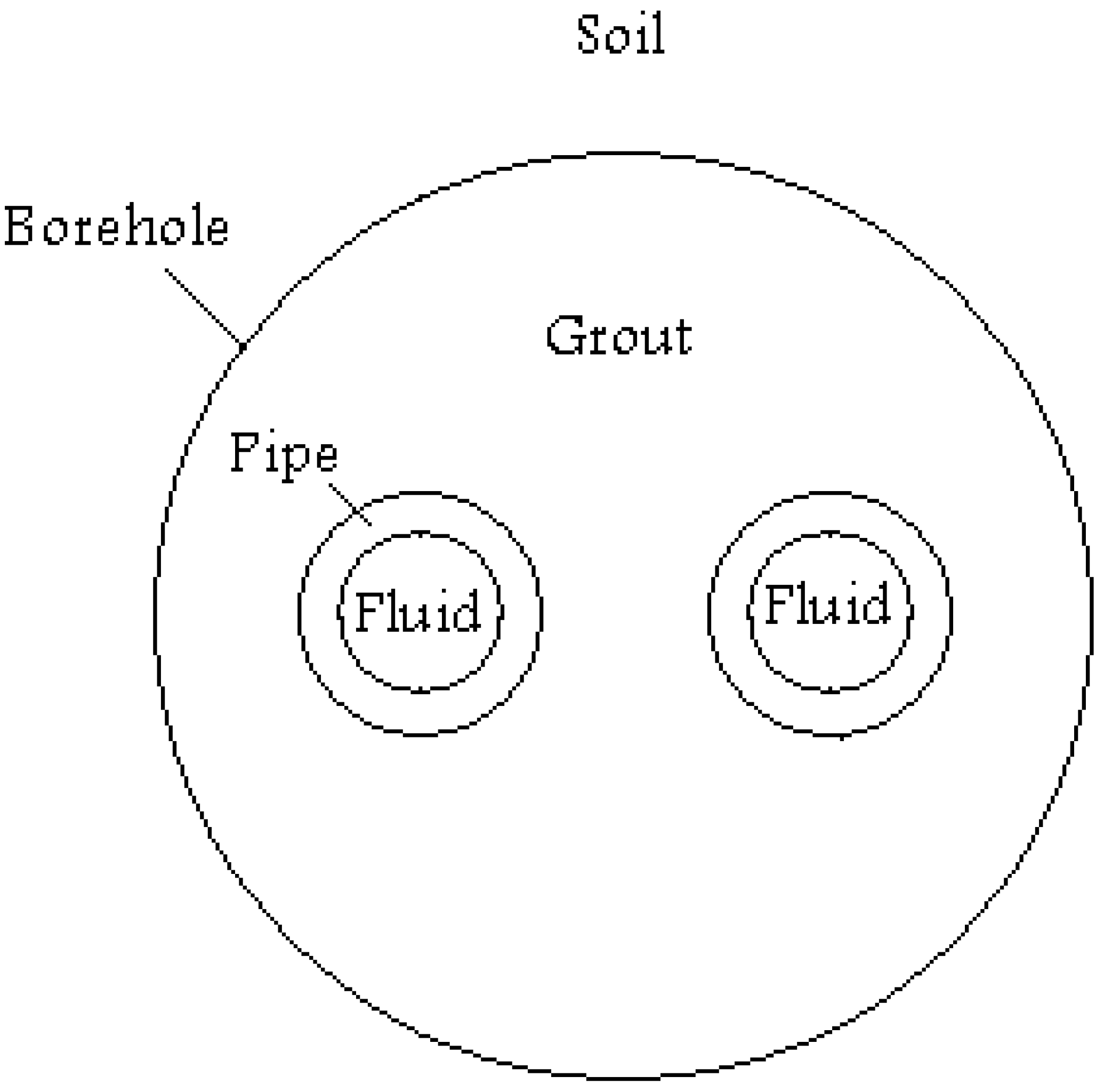
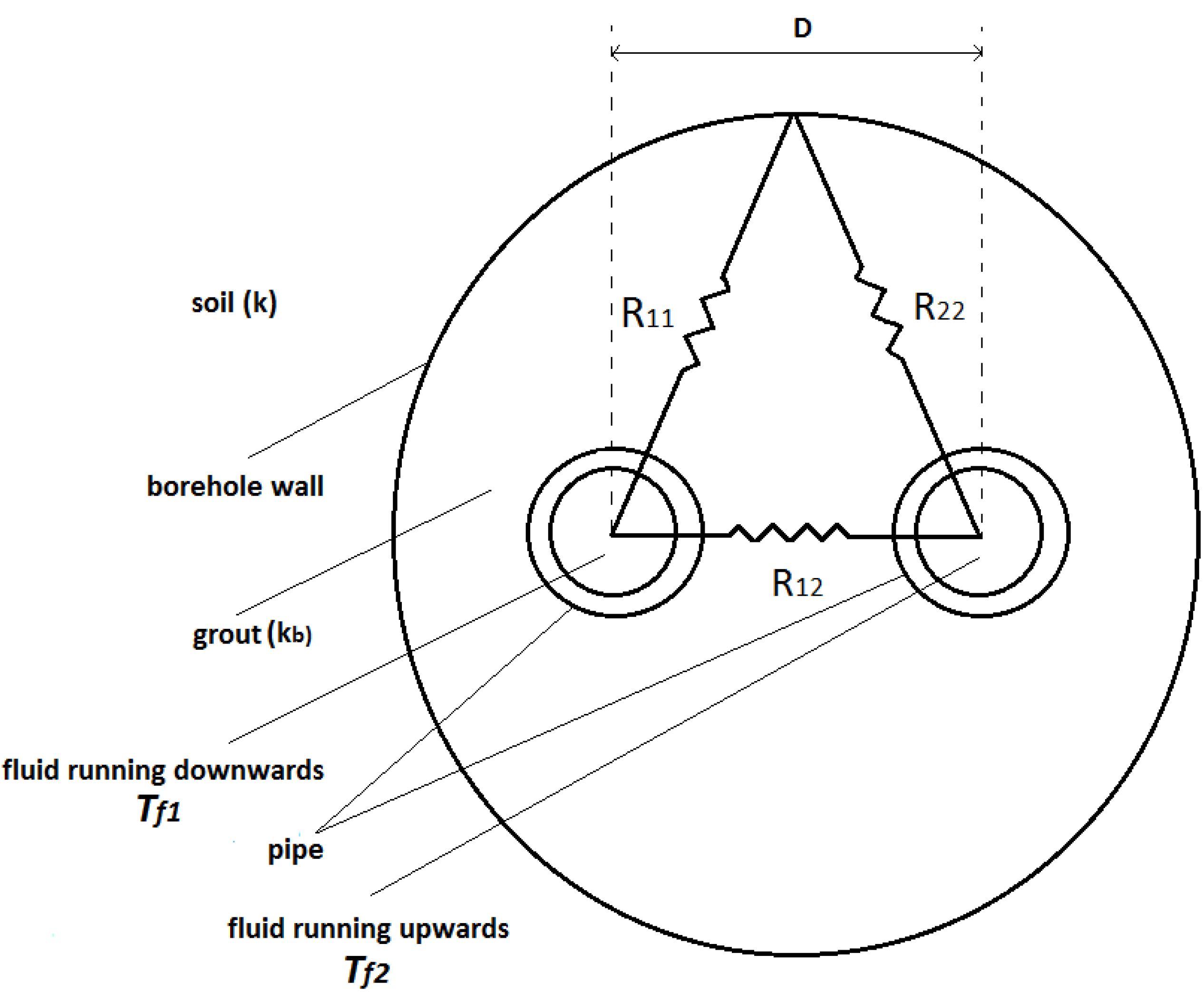
3.1.1. Heat Transfer inside the Borehole

The thermal analysis in the borehole seeks to define the inlet and outlet temperatures of the circulating fluid according to borehole wall temperature, its heat flow and the thermal resistance inside the borehole. The latter quantity is determined by thermal properties of the grouting material, the arrangement of flow channels and the convective heat transfer in the tubes. If the thermal resistance between the borehole wall and inner fluid is determined, the GHE fluid temperature can be calculated. Neglecting natural convection, moisture flow and freezing, the borehole thermal resistance can be calculated assuming steady-state heat conduction in the region between the circulating fluids and a cylinder around the borehole when the running time is greater than the critical time, that is Fo > 5, where Fo is the Fourier number ( Sustainability 05 02519 i006), and the impact of thermal capacity of objects inside the borehole can be neglected [11]. Such simplification has been proved approximate and convenient for most engineering analyses dealing with responses of more than a few hours [12].
In all analytical models for inside of borehole, the axial heat flows in the grout and pipe walls are considered negligible, as the borehole dimensional scale is small compared with the infinite extent of the ground beyond the borehole [13]. However, the fluid circulating through different legs of the U-tube exchanges heat with the surrounding ground and is of varying temperature along the tube. In particular, when the flow rate is low, there is a bigger temperature difference between the upward and downward channels which may result in thermal interference between the two channels and degrades efficiency of the GHE. Due to the U-tube structure, the heat conduction in the cross section is clearly two-dimensional, and the variation of the fluid temperature along the borehole length is in the third dimension.
In some models, such as the Equivalent Diameter method [14,15,16] and the Shape Factor method [17], the U-tube is conceived as a single pipe, and heat transfer in the borehole is approximated as a steady-state one-dimensional process. This oversimplified one-dimensional model is not capable of evaluating thermal interference among borehole legs, analyzing dynamic responses within a few hours, or the axial temperature gradient along the borehole. In the two-dimensional model [18], the effect of U-tube placement is accounted for in the heat conduction problem. The temperature of the fluid in the U-tube is defined by superposing two separate temperature responses caused by the heat fluxes per unit length from the two pipes of the U-tube. A quasi-three-dimensional model was proposed by Zeng et al. [19,20], taking into account the fluid axial convective heat transfer and thermal “short-circuiting” among U-tube legs. At the instance of symmetric disposal of the U-tube inside the borehole, the temperature profiles in the two pipes are reduced as:
Sustainability 05 02519 i001
where the dimensionless parameters are defined as:
Sustainability 05 02519 i002
where z denotes the direction along the tube, H the borehole length, Tf the circulating fluid temperature, Tb the borehole wall temperature, and Tf’ the temperature of the fluid entering the U-tube. Also, R11 and R22 are the thermal resistances between inlet and outlet legs of the U-tube and the borehole wall, respectively, and R12 is the thermal resistance between the inlet and outlet legs of the U-tube (Figure 2). These thermal resistances can be calculated analytically using the Multipole Method [18,21]. It is seen in Equation (1) that the Quasi-3-D model is able to reflect the variation of the temperature of the circulating fluid (Tf) along the tube (Z). Quasi-3-D models are preferred for design and analysis of GHEs, as they provide more accurate information on the heat flows inside the borehole.
Figure 2. Thermal resistances in the borehole.
Sustainability 05 02519 g002
Many of the models for heat transfer analysis inside the borehole are summarized in Table 1. Further improvements, such as accounting for thermal capacity of the borehole components to improve the precision of the resistance model, can be made to improve the accuracy of the model inside the borehole [22,23,24].
Table 1. Comparison of various methods in the heat analysis inside the borehole.
1D (Equivalent diameter) [14]1D (Shape factor) [17]2D [18]Quasi 3D [20]
U-tube disposalNYYY
Quantitative expressions of the thermal resistance in the cross-sectionNNYY
Thermal interferenceNNNY
Extinction between the entering and exiting pipesNNNY
Axial convection by fluid flowNNNY
Axial conduction in groutNNNN

3.1.2. Heat Transfer outside the Borehole

Several simulation models for the heat transfer outside the borehole are available. The main objective of heat transfer analysis outside the borehole is to determine the transient borehole surface temperature, which is the key to the heat transfer analysis inside the borehole. The models vary in the way the problem of heat conduction in the soil is solved and the way the interference between boreholes is treated.
In the analysis of GHE heat transfer, some complicating factors, such as groundwater movement [25] usually prove to be of minor importance and are analyzed separately. Therefore, the problem of heat transfer outside the borehole becomes a heat conduction problem. The general heat conduction equation in cylindrical coordinates appears in the following form:
Sustainability 05 02519 i003
where t denotes the time from the start of operation, α the thermal diffusivity of soil, and T the temperature of the ground. The first two terms on the left side of Equation (3) are the heat flux components in the radial (r) direction, the third and the fourth terms are related to the circumferential (φ) and axial (z) directions, respectively, and the fifth term relates to the heat generated in the control volume. The right side of Equation (3) represents the transient effects of heat conduction.
Unlike the area inside the borehole, heat conduction outside the borehole exhibits transient behavior. As a basic problem, the following assumptions are commonly made:
-
The ground is homogeneous in its thermal properties and initial temperature.
-
Moisture migration is negligible.
-
Thermal contact resistance is negligible between the pipe and grout and between the grout and soil.
-
The effect of ground surface is negligible for the initial 5–10 years (depending on the borehole depth).
Due to its minor order, heat transfer in the axial direction along the borehole, which accounts for the heat flux across the ground surface and down to the bottom of the borehole, is considered negligible. This assumption is valid for a length of the borehole distant enough from the borehole top and bottom. Additionally, heat transfer in the circumferential direction is negligible in this model assuming a single borehole. Therefore, the heat transfer is usually modeled with a one-dimensional analysis assuming that the axial and circumferential heat flows are negligible.
The earliest approaches to calculating the heat transfer in the soil surrounding a GHE is Kelvin’s line-source model, i.e., the infinite line-source, which uses Fourier’s law of heat conduction [26]. In the line-source theory, the borehole is assumed as an infinite line source of heat in the ground, which is regarded as an infinite medium with an initial uniform temperature. This model derives an analytical relation for the temperature excess of the soil, assuming a constant heat flow rate on the borehole wall (here, the line source). Another one-dimensional model based on Fourier’s law of heat conduction is the cylindrical source model [27]. In this model, the borehole is assumed to be a cylindrical pipe with infinite length buried in the ground. The governing equation for this model can be solved analytically for either a constant borehole surface temperature or a constant heat transfer rate from the borehole to the ground. At long distances and after a long time, the two models are equivalent. However, the line source model is more popular, since its solution is easier to evaluate, and it is numerically more stable [28]. To make the analytical results obtained by the line source theory for analysis outside of the borehole more accurate and comparable to numerical ones, several studies have focused on improvements [29,30,31,32]. Hellström [18], Kavanaugh [33], Bernier et al. [34] and Hikari et al. [35] focus on improvements on cylindrical source solution.
In both analytical models of Kelvin’s theory and the cylindrical source model, the borehole depth is considered infinite, and the axial heat flow along the borehole depth is assumed negligible. Furthermore, when time tends to infinity, the temperature rise of the Kelvin’s theory for an infinite line source tends to infinity, making the infinite model weak for describing heat transfer mechanism in long time steps. Therefore, they can only be used for short time range of operations of GCHP systems. To take into account axial temperature changes for boreholes with finite lengths and in long durations, Eskilson’s approach to the problem of determining the temperature distribution around a borehole is based on combination of analytical and numerical solution techniques. Eskilson [36] applies a numerical finite-difference method to the transient radial-axial heat conduction equation for a single borehole. Based on the Eskilson’s model [36], Zeng et al. [19,37] and Diao et al. [38] present an analytical solution to the transient finite line-source problem considering the effects of the finite borehole length and the ground surface as an isothermal boundary. They assume no temperature change on the ground surface (by superimposing an identical mirror borehole above the ground surface with negative strength). With these assumptions, the solution of the temperature excess for a heating rate per length of the constant source ( Sustainability 05 02519 i004) is:
Sustainability 05 02519 i005
where T is the temperature of the ground at radial distance r, axial distance z, and at time t, T0 is the initial temperature of the ground, and q’ is the heat flow rate per unit length of the borehole. Note that in Equation (4), the heat flow rate per unit length of the borehole is assumed constant along the borehole and steady throughout the operation time. Using this solution as a basic step pulse allows the calculation of temperature response to any load varying with time by considering piecewise constant heat extractions/rejections and superposing them in time as a series of load steps [36]. However, for long time periods, this process becomes computationally intensive. Some authors have focused on introducing efficient algorithms that lower the number of time steps [34,39], while others have used the convolution theorem in the frequency domain using fast Fourier transform to lower the computational burden of hourly temperature evaluations related to a time-varying heat load [28].
In the analytical models presented above, a number of assumptions are employed in order to simplify the complicated governing equations. In time varying heat transfer rates and the influence of surrounding boreholes on both long and short time scales, analytical methods are not as suitable as numerical methods. However, due to their much shorter computation times, they are still used widely in designing GHEs.

3.2. Numerical Models

System simulation models require the ability to operate at short time scales, often less than one minute. Therefore, the dynamic response of the grout material inside the borehole should be considered. This is possible when the model is solved using numerical techniques. Numerical methods have also been used extensively for evaluating the heat conduction inside the borehole and the soil surrounding it [11,40,41,42,43,44,45,46,47,48,49,50]. In addition to short time step solution, numerical techniques are advantages over the available analytical ones due to accounting for all the terms in the conduction equation [Equation (3)] and the ability to apply transient boundary conditions on the model such as the surface, borehole wall and the inlet temperature boundaries. Model additions, such as accounting for moisture migration in the soil and ground stratification, are easier to be made in a numerical model than the analytical ones.
One of the disadvantages of numerical approaches is their computation time for long-term system performance. The diameters of the U-tubes in the borehole are fairly small, on the order of 102 m, while the size of the solution domain, which depends on the duration of system operation and its heating/cooling load, is approximately on an order of 10 m, making the domain extremely disproportionate. As a result, a large number of mesh elements is required for simulation of a single borehole and its surrounding soil. To achieve an inaccuracy of 2% or less for the steady state heat transfer analysis of boreholes, a minimum number of approximately 18 elements describing any circular shape of a horizontal cross section is needed [51]. In modelling the soil surrounding the borehole, a domain of a certain size can work well for one model, while it can be too small for another model requiring more boreholes, longer system performance durations or higher heating injection/removal rates. At the outer edge of the domain, a constant far-field temperature condition equal to the initial temperature is often applied. The sensitivity of the solution results to this boundary should always be examined and avoided by increasing the size of the domain. In three-dimensional modeling of a borehole system with typical flow velocities, a vertical element size of 2 m or less should often be applied to avoid inaccuracies of greater than 2% [51].
The temperature gradient in the domain between the borehole wall and the far field changes gradually from large to small. Therefore, to reduce computer memory and computational time, the size of the mesh cells is often chosen based on this gradual change. Furthermore, the symmetry about the GHE can be used to save computation time. In such cases, the symmetric portion of the solution domain is replaced by an adiabatic wall boundary condition on the symmetry line. Applying all these techniques, a three-dimensional 15 m × 15 m × 60 m domain may require mesh sizes of the order of 1,000,000 elements to simulate multiple boreholes of 50 m length.
Due to these limitations, several available models are limited to a two-dimensional (2D) description of the domain [41,50]. Factors such as vertical heat transport in and outside the borehole, different ground layers, the vertical gradient of the undisturbed ground temperature, the transient fluid transport inside the tubes, the thermal short-circuiting between the upward and downward tubes, and the correct boundary conditions at the upper and lower boundaries are generally ignored in the 2D models. Some models describe the system in a three-dimensional domain by reducing the number of mesh elements, but this approach can result in lower accuracy. There are also several numerical techniques available in different numerical approaches which can be used to reduce the computation time [23,24,51].
To evaluate the long-term temperature response in the soil surrounding multiple borehole systems, a numerical finite volume method in a two-dimensional meshed domain is used previously [52]. The effect of installing GHEs in the ground and the temperature rise in the soil over the long-term, for a period of five years, is considered. A transient periodic heat flux is assumed on the borehole wall reflecting the annual variation of heat storage/removal in the ground. When monthly bin weather information, building needs and heat pump performance and efficiency data are available, this periodic heat flux can be calculated and used as a heat boundary condition in the numerical model. It is assumed that flow rate and the inlet temperature of the circulating fluid running in the U-tube inside the borehole will be adjusted according to the building heating needs. The five-year simulation of the system shows that for a system that has a balanced heat injection and extraction into the soil, if the borehole spacing and the heat injection/extraction rate are designed within acceptable limits, there will not be any temperature increase or decrease in the soil surrounding the system. Any temperature rise or decrease in the soil surrounding the GHE that is noticed after the first year operation needs to be compensated for during the second year operation so that the system can operate sustainably.
One limitation in the previous studies [52] is using a heat flux boundary condition on the borehole wall. As mentioned previously, using a heat flux boundary condition can cause the temperature of the ground to rise infinitely without a stop in system operation. In reality, if the temperature of the soil surrounding a borehole becomes close to or higher than the inlet temperature of the circulating fluid exiting the heat pump, the system will not be able to deliver the desired heat to the ground and will automatically stop operating until the heat around it is dissipated away and the temperature drops to a lower value. In order to overcome such a limitation, the periodic heat boundary on the borehole wall can be replaced with a temperature boundary or the heat boundary can be updated at short time steps with respect to the soil temperature. This is possible if the heat transfer model for outside of the borehole is coupled to the model inside the borehole.

3.3. Some Modeling Limitations

One limitation in most of the previous studies is the assumption of uniform heat input along the borehole length to the ground, either when the borehole is assumed as a cylinder or a line source of heat. In order to determine the borehole heat delivery/removal profile along the borehole, the heat transfer model outside the borehole should be coupled to the one inside the borehole. In a recent study, Koohi-Fayegh and Rosen [53] use the analytical quasi-three-dimensional solution to the heat transfer problem of the U-tube configuration inside the borehole. This model evaluates the temperature of the circulating fluid along the borehole length and is used in the model for outside the borehole to calculate the heat delivery/removal along the borehole caused by the temperature difference between the circulating fluid and the borehole wall temperature. The heat delivery/removal is implemented as the heat boundary condition in the analytical line source with finite length as well as in a three-dimensional finite volume model [54,55]. The results show that due to the higher heating strength at the top end of the boreholes (about 3% total length), the possibility of thermal interaction at the top of the borehole is at its highest, and it decreases along the borehole length as the heat flux from the borehole wall into the soil decreases. Therefore, with the objective of limiting boreholes’ operations and sizes in order to prevent their thermal interaction, the top length of the boreholes is the critical area. It can be concluded that using a uniform heat flux along the borehole is only accurate for the middle length of the boreholes, and moving any further to the top or bottom of the borehole, the temperature rise evaluations become relatively inaccurate.
Another limitation in the previous studies is the assumption of steady borehole wall temperature during system operation. When calculating the heat input to the ground, it becomes clear that it varies with the borehole wall temperature. Although the soil temperature at the borehole wall rises as the system operates, it is often assumed that the soil temperature at the borehole wall is constant throughout the operation period. This assumption ignores the drop in heat injection strength when the borehole wall temperature increases and, therefore, underestimates the inlet temperature of the circulating fluid that is required to meet the heat injection needs of the system. Yang et al. [56] propose and develop an updated two-region vertical U-tube GHE analytical model coupling two solutions for inside and outside the borehole with transient temperature of borehole wall. In the fewer cases of multiple boreholes, superposition of the temperature excesses resulted from individual boreholes seems to be the most popular solution in analytical approaches. In numerical approaches, the boundary condition that plays the role of heat delivery/removal is a heat boundary type that, regardless of being constant or variable based on the building needs, does not reflect the drop in the heat injection/removal strength when temperature of the soil around the borehole increases/decreases by its own performance or another nearby system’s performance. This assumption forces the system to deliver a desired amount of heat to the ground regardless of the ground temperature. In reality, the amount of heat delivered to the ground is driven by the temperature difference between the circulating fluid and the ground temperature. In some cases, the assumption of constant borehole wall temperature is acceptable considering how the conduction problem is simplified. However, when determining how thermal interaction between two operating GHEs can affect their performance, the effect of the transient borehole wall temperature on their heat delivery strength and inlet fluid temperature becomes a very important factor. Therefore, this model is only able to illustrate the variation of the heat delivery/removal strength when the heat flow rate is low and the temperature changes at the borehole wall are small.
In order to account for higher heat flow rates or thermal interaction between multiple boreholes, the model should be modified to include the transient value of borehole wall temperature. Thus, the non-uniform heat flow rate along the borehole wall becomes transient as well. A model is needed that is able to not only estimate how heat flows in the region surrounding GHEs, but also how a temperature rise in the soil surrounding a borehole caused by the system itself or a neighboring geothermal system can interfere with its heat delivery strength.

3.4. Other Modeling Aspects

Performing energy and moisture balances at the ground surface involves very complex processes, taking into account solar radiation, cloud cover, surface albedo, ambient air temperature and relative humidity, rainfall, snow cover, wind speed and evapotranspiration. Such details provide a proper account of the renewable energy resource. However, due to the complexity of adding all the above heat fluxes in a numerical model, some studies assume the ground surface temperature variation at the ground surface to take the form of a sine wave or Fourier series [57,58,59,60], while, in most analytical approaches, the ground surface boundary is assumed to have a constant temperature equal to the soil temperature deep in the ground (by superimposing an identical mirror borehole above the ground surface with negative strength). Moreover, some studies simplify the problem further and assume an adiabatic boundary condition at the ground surface.
Neglecting the existence of moisture in the soil, the heat flux is described via the conduction heat flow. The coupled heat and moisture flow in a soil system is described with a thermal energy balance coupled with a mass balance. This adds to the complication of the problem since the complete model contains a set of transient simultaneous partial differential equations with many soil parameters that are not readily available. Research shows that the effects of moisture migration are not significant to the operation of a vertical GHE; it is expected that these effects are more pronounced with a horizontal GHE. This is because natural variations of temperature and moisture near the ground surface and operation of the HGHE may create a potentially greater moisture movement. During the cooling season, migration of soil moisture away from the GHE may lead to a drastic drop in soil thermal conductivity and consequently a significantly reduced heat transfer, which has a devastating effect on GHE performance. Therefore, although moisture migration effects can be neglected in early stages of design or conceptual development, not considering them in long-term operation of GCHP systems makes it impossible to assess the performance and potential failure of these systems [61]. Some studies focus on the thermal interaction between the circulating fluid and soil, taking into account heat flow with moisture transfer in the soil [40,43,61,62].
A further complication in the design of ground-coupled heat pump systems is the presence of groundwater. Due to the difficulties encountered both in modeling and computing the convective heat transfer and in learning about the actual groundwater flow in engineering practice, each of the methods presented in the previous sections is based on Fourier’s law of heat conduction and neglect the effects of groundwater flow in carrying away heat. Where groundwater is present, flow will occur in response to hydraulic gradients, and the physical process affecting heat transfer in the ground is inherently a coupled one of heat diffusion (conduction) and heat advection by moving groundwater [63]. Similar to the models discussed in the previous sections, here as well, the objective is to evaluate the temperature response in the soil surrounding GHEs. The effect of ground water is analyzed using numerical [26,64,65,66] and analytical approaches [63,67].

4. Conclusions

An assessment of the available analytical models demonstrates that they are not capable of estimating the heat delivery/removal strength when the soil surrounding them experiences a temperature rise. In the current study, it is shown that the effect of the temperature rise in the soil surrounding boreholes is not negligible. The distance between two boreholes or two systems of boreholes, the heat flux from the borehole wall and the time of system operation all affect directly the amount of thermal interaction between the systems. However, the effect of these parameters on system operation and heat delivery/removal rate can only be studied in models that account for the change in the borehole wall temperature.
As mentioned in the previous section, in order to account for the sustainability of the system and heat pump efficiency when thermal interaction among boreholes occur, it is important to develop and utilize models that account for the drop in heat delivery strength when the borehole wall temperature increases during the operation time or by another nearby operating system. As a result, the inlet temperature of the circulating fluid needs to be adjusted to a higher/lower one to maintain the heat delivery/removal needs of the system. This analysis is important since ground heat exchangers are coupled to a heat pump that can only work within a certain temperature lift and inlet and outlet circulating temperature ranges. If a system is able to deliver a certain amount of heat to the ground, the increase in the inlet circulating temperature due to temperature rise in the soil caused by a nearby system reflects how thermal interaction affects the sustainability of the system. Furthermore, simulation of heat exchange processes within the system and surrounding environment through local scale assessment, simulation of migration of thermal plumes into the hydrogeological environment through intermediate and regional scale assessment will help gain an estimation of ecological impacts.

Acknowledgments

The support provided by the Ontario Ministry of Environment through its Best in Science program is gratefully acknowledged.

Conflict of Interest

The authors declare no conflict of interest.

References

  1. Geothermal Heat Pump Consortium. Available online: http://energy.nstl.gov.cn/MirrorResources/902/index.html/ (accessed on 1 November 2011).
  2. Fisheries and Oceans Canada, Ontario-Great Lakes Area (DFO-OGLA). Fish Habitat and Fluctuating Water Levels on the Great Lakes. Available online: http://www.dfo-mpo.gc.ca/regions/central/pub/factsheets-feuilletsinfos-on/t2-eng.htm (accessed on 1 November 2011).
  3. Markle, J.M.; Schincariol, R.A. Thermal plume transport from sand and gravel pits: Potential thermal impacts on cool water streams. Hydrology 2007, 338, 174–195. [Google Scholar]
  4. York, K.P.; Sarwar Jahangir, Z.M.G.; Solomon, T.; Stafford, L. Effects of a Large Scale Geothermal Heat Pump Installation on Aquifer Microbiota. In Proceedings of the Second International Conference on Geothermal Heat Pump systems at Richard Stockton College, Pomona, NJ, USA, 16–17 March 1998.
  5. Ferguson, G.; Woodbury, A.D. Thermal sustainability of groundwater-source cooling in Winnipeg, Manitoba. Can. Geothechnical J. 2005, 42, 1290–1301. [Google Scholar]
  6. Ferguson, G.; Woodbury, A.D. Observed thermal pollution and and post-development simulations of low-temperature geothermal systems in Winnipeg, Canada. Hydrogeology 2006, 14, 1206–1215. [Google Scholar]
  7. Younger, P.L. Ground-coupled heating-cooling systems in urban areas: How sustainable are they? Bull. Sci. Technol. Soc. 2008, 28, 174–182. [Google Scholar]
  8. Andrushuk, R.; Merkel, P. Performance of ground source heat pumps in Manitoba. Available online: http://www.hydro.mb.ca/regulatory_affairs/electric/gra_2012_2013/Appendix_38.pdf (accessed on 1 November 2011).
  9. Ferguson, G. Unfinished business in geothermal energy. Ground Water 2009, 47, 167–167. [Google Scholar]
  10. Eskilson, P.; Claesson, J. Simulation model for thermally interacting heat extraction boreholes. Numer. Heat Transf. 1988, 13, 149–165. [Google Scholar]
  11. Jun, L.; Xu, Z.; Jun, G.; Jie, Y. Evaluation of heat exchange rate of GHE in geothermal heat pump systems. Renew. Energy 2009, 34, 2898–2904. [Google Scholar]
  12. Yavuzturk, C. Modeling of vertical ground loop heat exchangers for ground source heat pump systems. Ph.D. thesis, Oklahoma State University, Oklahoma, OK, USA, 1999. [Google Scholar]
  13. Bose, J.E.; Parker, J.D.; McQuiston, F.C. Design/Data Manual for Closed-Loop Ground Coupled Heat Pump Systems; Oklahoma State University for ASHRAE: Stillwater, OK, USA, 1985. [Google Scholar]
  14. Claesson, J.; Dunand, A. Heat Extraction from the Ground by Horizontal Pipes: A Mathematical Analysis; Swedish Council for Building Research: Stockholm, Sweden, 1983. [Google Scholar]
  15. Gu, Y.; O’Neal, D.L. Development of an equivalent diameter expression for vertical U-tube used in ground-coupled heat pumps. ASHRAE Trans. 1998, 104, 347–355. [Google Scholar]
  16. Gu, Y.; O’Neal, D.L. Modeling the effect of backfills on U-tube ground coil performance. ASHRAE Trans. 1998, 104, 356–365. [Google Scholar]
  17. Paul, N.D. The effect of grout conductivity on vertical heat exchanger design and performance. Master Thesis, South Dakota State University, Madison, SD, USA, 1996. [Google Scholar]
  18. Hellström, G. Ground heat storage: Thermal analyses of duct storage systems. Ph.D. thesis, Department of Mathematical Physics, University of Lund, Lund, Sweden, 1991. [Google Scholar]
  19. Zeng, H.Y.; Diao, N.R.; Fang, Z. Efficiency of vertical geothermal heat exchangers in ground source heat pump systems. J. Therm. Sci. 2003, 12, 77–81. [Google Scholar] [CrossRef]
  20. Zeng, H.Y.; Diao, N.R.; Fang, Z. Heat transfer analysis of boreholes in vertical ground heat exchangers. Int. J. Heat Mass Transf. 2003, 46, 4467–4481. [Google Scholar]
  21. Claesson, J.; Hellström, G. Multipole method to calculate borehole thermal resistances in a borehole heat exchanger. HVAC&R Res. 2011, 17, 895–911. [Google Scholar]
  22. Bauer, D.; Heidemann, W.; Muller-Steinhagen, H.; Diersch, H.-J.G. Thermal resistance and capacity models for borehole heat exchangers. Int. J. Energy Res. 2011, 35, 312–320. [Google Scholar]
  23. Al-Khoury, R.; Bonnier, P.G.; Brinkgreve, R.B.J. Efficient finite element formulation for geothermal heating systems, Part I: Steady state. Int. J. Numer. Methods Eng. 2005, 63, 988–1013. [Google Scholar] [CrossRef]
  24. Al-Khoury, R.; Bonnier, P.G. Efficient finite element formulation for geothermal heating systems, Part II: Transient. Int. J. Numer. Methods Eng. 2006, 67, 725–745. [Google Scholar]
  25. Chiasson, A.D.; Rees, S.J.; Spitler, J.D. A preliminary assessment of the effects of groundwater flow on closed-loop ground-source heat pump systems. ASHRAE Trans. 2000, 106, 380–393. [Google Scholar]
  26. Ingersoll, L.R.; Zobel, O.J.; Ingersoll, A.C. Heat Conduction with Engineering, Geological, and other Applications, rev. ed.; University of Wisconsin Press: Madison, WI, USA, 1954. [Google Scholar]
  27. Carslaw, H.S.; Jaeger, J.C. Conduction of Heat in Solids; Claremore Press: Oxford, UK, 1946. [Google Scholar]
  28. Marcotte, D.; Pasquier, P. Fast fluid and ground temperature computation for geothermal ground-loop heat exchanger systems. Geothermics 2008, 37, 651–665. [Google Scholar]
  29. Ingersoll, L.R.; Plass, H.J. Theory of the ground pipe heat source for the heat pump. ASHVE Trans. 1948, 47, 339–348. [Google Scholar]
  30. Hart, D.P.; Couvillion, R. Earth Coupled Heat Transfer; National Water Well Association: Dublin, OH, USA, 1986. [Google Scholar]
  31. Lamarche, L.; Beauchamp, B. A new contribution to the finite line source model for geothermal boreholes. Energy Build. 2007, 39, 188–198. [Google Scholar]
  32. Cui, P.; Yang, H.; Fang, Z.H. Heat transfer analysis of ground heat exchangers with inclined boreholes. Appl. Therm. Eng. 2006, 26, 1169–1175. [Google Scholar]
  33. Kavanaugh, S.P. A design method for commercial ground-coupled heat pumps. ASHRAE Trans. 1995, 101, 1088–1094. [Google Scholar]
  34. Bernier, M.; Pinel, A.; Labib, P.; Paillot, R. A multiple load aggregation algorithm for annual hourly simulations of GCHP systems. HVAC&R Res. 2004, 10, 471–487. [Google Scholar]
  35. Hikari, F.; Ryuichi, I.; Takashi, I. Improvements on analytical modeling for vertical U-tube ground heat exchangers. Geotherm. Resour. Counc. Trans. 2004, 28, 73–77. [Google Scholar]
  36. Eskilson, P. Thermal analysis of heat extraction boreholes. Doctoral thesis, Department of Mathematical Physics, University of Lund, Lund, Sweden, 1987. [Google Scholar]
  37. Zeng, H.Y.; Diao, N.R.; Fang, Z. A finite line-source model for boreholes in geothermal heat exchangers. Heat Transf. Asian Res. 2002, 31, 558–567. [Google Scholar] [CrossRef]
  38. Diao, N.R.; Zeng, H.Y.; Fang, Z.H. Improvement in modeling of heat transfer in vertical ground heat exchangers. HVAC&R Res. 2004, 10, 459–470. [Google Scholar]
  39. Yavuzturk, C.; Spitler, J. A short time step response factor model for vertical ground loop heat exchangers. ASHRAE Trans. 1999, 105, 475–485. [Google Scholar]
  40. Mei, V.C.; Baxter, V.D. Performance of a ground-coupled heat pump with multiple dissimilar U-tube coils in series. ASHRAE Trans. 1986, 92, 22–25. [Google Scholar]
  41. Yavuzturk, C.; Spitler, J.D.; Rees, S.J. A transient two-dimensional finite volume model for the simulation of vertical U-tube ground heat exchangers. ASHRAE Trans. 1999, 105, 465–474. [Google Scholar]
  42. Yavuzturk, C.; Spitler, J.D. Field validation of a short time step model for vertical ground-loop heat exchangers. ASHRAE Trans. 2001, 107, 617–625. [Google Scholar]
  43. Muraya, N.K. Numerical modeling of the transient thermal interference of vertical U-tube heat exchangers. Ph.D. Thesis, Texas A&M University, College Station, TX, USA, 1995. [Google Scholar]
  44. Kavanaugh, S.P. Simulation and experimental verification of vertical ground coupled heat pump systems. Ph.D. Thesis, Oklahoma State University, Oklahoma, OK, USA, 1985. [Google Scholar]
  45. Rottmayer, S.P.; Beckman, W.A.; Mitchell, J.W. Simulation of a single vertical U-tube ground heat exchanger in an infinite medium. ASHRAE Trans. 1997, 103, 651–658. [Google Scholar]
  46. Lee, C.K.; Lam, H.N. Computer simulation of borehole ground heat exchangers for geothermal heat pump systems. Renew. Energy 2008, 33, 1286–1296. [Google Scholar] [CrossRef]
  47. Li, Z.; Zheng, M. Development of a numerical model for the simulation of vertical U-tube ground heat exchangers. Appl. Therm. Eng. 2009, 29, 920–924. [Google Scholar] [CrossRef]
  48. He, M.; Rees, S.; Shao, L. Simulation of a Domestic Ground Source Heat Pump System Using a Transient Numerical Borehole Heat Exchanger Model. In Proceedings of 11th International Building Performance Simulation Association Conference, Glasgow, Scotland, 27–30 July 2009; pp. 607–614.
  49. Fang, Z.H.; Diao, N.R.; Cui, P. Discontinuous operation of geothermal heat exchangers. Tsinghua Sci. Technol. 2002, 7, 194–197. [Google Scholar]
  50. Austin, W.A.; Yavuzturk, C.; Spitler, J.D. Development of an in situ system for measuring ground thermal properties. ASHRAE Trans. 2000, 106, 356–379. [Google Scholar]
  51. Bauer, D.; Heidemann, W.; Diersch, H.-J.G. Transient 3D analysis of borehole heat exchanger modeling. Geothermics 2011, 40, 250–260. [Google Scholar] [CrossRef]
  52. Koohi-Fayegh, S.; Rosen, M.A. Long-term Study of Thermal Interaction of Vertical Ground Heat Exchangers with Seasonal Heat Flux Variation. In Proceedings of 11th International Conference on Sustainable Technologies, Vancouver, BC, Canada, 2–5 September 2012.
  53. Koohi-Fayegh, S.; Rosen, M.A. Thermally Interacting Multiple Boreholes with Variable Heating Strength. In Proceedings of eSim Conference, Halifax, NS, Canada, 2–3 May 2012.
  54. Koohi-Fayegh, S.; Rosen, M.A. A Numerical Approach to Assessing Thermally Interacting Multiple Boreholes with Variable Heating Strength. In Proceedings of 1st World Sustainability Forum, 1–30 November 2011.
  55. Koohi-Fayegh, S.; Rosen, M.A. On thermally interacting multiple boreholes with variable heating strength: Comparison between analytical and numerical approaches. Sustainability 2012, 4, 1848–1866. [Google Scholar] [CrossRef]
  56. Yang, W.; Shi, M.; Liu, G.; Chen, Z. A two-region simulation model of vertical U-tube ground heat exchanger and its experimental verification. Appl. Energy 2009, 86, 2005–2012. [Google Scholar] [CrossRef]
  57. Salah El-Din, M.M. On the heat flow into the ground. Renew. Energy 1999, 18, 473–490. [Google Scholar] [CrossRef]
  58. Mihalakakou, G. On estimating ground surface temperature profiles. Energy Build. 2002, 34, 251–259. [Google Scholar] [CrossRef]
  59. Mihalakakou, G.; Lewis, J.O. The influence of different ground covers on the heating potential of the earth-to-air heat exchangers. Renew. Energy 1996, 7, 33–46. [Google Scholar] [CrossRef]
  60. Jacovides, C.P.; Mihalakakou, G.; Santamouris, M.; Lewis, J.O. On the ground temperature profile for passive cooling applications in buildings. Solar Energy 1996, 57, 167–175. [Google Scholar] [CrossRef]
  61. Leong, W.H.; Tarnawski, V.R. Effects of Simultaneous Heat and Moisture Transfer in Soils on the Performance of a Ground Source Heat Pump System. In Proceedings of ASME-ATI-UIT Conference on Thermal and Environmental Issues in Energy Systems, Sorrento, Italy, 16–19 May 2010.
  62. Piechowski, M. Heat and mass transfer model of a ground heat exchanger: Theoretical development. Int. J. Energy Res. 1999, 23, 571–588. [Google Scholar] [CrossRef]
  63. Sutton, M.; Nutter, D.; Couvillion, R. A ground resistance for vertical bore heat exchangers with groundwater flow. J. Energy Resour. Technol. 2003, 125, 183–189. [Google Scholar] [CrossRef]
  64. Gehlin, S.E.A.; Hellström, G. Influence on thermal response test by groundwater flow in vertical fractures in hard rock. Renew. Energy 2003, 28, 2221–2238. [Google Scholar] [CrossRef]
  65. Nam, Y.; Ooka, R.; Hwang, S. Development of a numerical model to predict heat exchange rates for a ground-source heat pump system. Energy Build. 2008, 40, 2133–2140. [Google Scholar] [CrossRef]
  66. Hecht-Mendez, J.; Molina-Giraldo, N.; Blum, P.; Bayer, P. Evaluating MT3DMS for heat transport simulation of closed geothermal systems. Ground Water 2010, 48, 741–756. [Google Scholar] [CrossRef]
  67. Diao, N.R.; Li, Q.; Fang, Z.H. Heat transfer in ground heat exchangers with groundwater advection. Int. J. Therm. Sci. 2004, 43, 1203–1211. [Google Scholar] [CrossRef]

