1. Introduction
Large cities around the world are suffering from traffic congestion. Governments have adopted numerous measures to deal with this problem, such as Intelligent Transportation Systems (ITS) and travel demand management. Technologies like ITS could help to enhance road capacity, which of course will be effective to some extent. However, when the city keeps sprawling, congestion will come back again. A green transportation system composed of transit, busses and bicycles could be a significant alleviate to traffic congestion. Urban rail transit with its distinctive features, occupies a leading and unshakeable position in the urban public transport. Based on the understanding that ridership forecasting is the essential component of the transit project development process, a relatively high transit ridership forecasting accuracy would be of great significance to the improvements of public transport service level and urban transport environment.
The fundamental process of travel demand forecasting is analyzing the relationship between travel generation, distribution and Traffic Analysis Zone (TAZ) features. Based on the relationship and forecasted future TAZ features, future travel generation and distribution could be predicted [
1,
2,
3]. Thus, reasonable delineated TAZ is a necessary foundation of successful forecasting.
However, due to the distinctive features of urban transit system, TAZs in transit ridership forecasting should not be the same as comprehensive transport demand forecasting, in order to distinct them, come up with a new definition: Transit Traffic Analysis Zone (TTAZ), the features of which will be discussed later through the deficiency analysis of current TAZ delineating methods combined with transit travel characteristic analysis.
1.1. Literature Review
Four-step forecasting and sketch-level forecasting are the most common methods currently, and there are two “TTAZ” delineating methods correspondingly, which is called “catchment area” in sketch-level forecasting.
1.1.1. TTAZ Delineating Method in Four-Step Forecasting
Currently, when using four-step method in transit ridership forecasting, generally follows the TAZ delineated for comprehensive travel demand forecasting, deciding the boundary of TAZs qualitatively through the nature of land use, population distribution, administrative division, natural landscape, road network and some other factors. Obeying the following rules [
4,
5,
6]:
- (1)
Try to guarantee the consistency of features like land use, economy and society in one TAZ.
- (2)
Try to use natural barriers like railway and river as boundaries, avoiding natural or manmade barriers in TAZs.
- (3)
Try to delineate regular shaped TAZs, avoiding narrow shape.
- (4)
Pay attention to the road network. Try to guarantee that the TAZ centroids are on network node (intersections and roads).
- (5)
Try to put both sides of one road in the same TAZ.
- (6)
Trip generation in one TAZ should not exceed 10%–15% of all TAZs.
In recent years, scholars conducted researches on how to delineating TAZs in a more scientific way: Zhao Jinhuan and Li Wenquan [
7] classified the TAZs by fuzzy clustering based on the correlation between TAZ features and traffic characteristics; Ma Chaoqun and Wang Rui
et al [
8] combined with passenger travel characteristics and city size, come up with a TAZ radius calculation method based on the percentage of trips within TAZ; Cambridge Systematics, Inc. and AECOM Consult proposed the concept of dynamic delineating method based on the mixed land use in urban areas.
1.1.2. Catchment Area Delineating Method in Sketch-Level Forecasting
The “Traffic Analysis Zone” in sketch-level forecasting is delineated by drawing a circle to the station as the center, called catchment area. The radius of the circle was decided by walking distance to transit stations, scholars come up with different radiuses varying from 400 m (0.25 mile) to 800 m (0.5 mile) based on different ideas, and the most commonly used one is 800 m (0.5 mile) [
9,
10,
11,
12,
13,
14]. Some scholars take feeder busses and bikes into account, and the range of radiuses they came up with is relatively larger, from 400 m (0.25 mile) to 3200 m (2 mile) [
15,
16,
17,
18].
In recent years, Clayton lane and AICP come up with the concept of “exclusive station area” in order to solve the problem of catchment area overlapping [
19]; Javier Gutiérrez presented distance-decay weighted regression around transit stations in order to reflect the relationship between passenger flow and land use more precisely [
20].
1.2. Paper Structure
The remainder of the paper is structured as follows:
Section 2 analyzes the deficiencies of current “TTAZ” delineating method in four-step forecasting and sketch-level forecasting combine with transit travel characteristics;
Section 3, introduced Thiessen Polygon into TTAZ delineating according to the conclusions drawn from
Section 2. Beijing was then taken as an example to delineate TTAZs, followed by a preliminary spatial analysis;
Section 4 summarized the conclusion of this paper and made an outlook of future research.
2. Current Delineating Method of Transit Traffic Analysis Zone
2.1. Deficiencies of TTAZ in Four-Step Forecasting
Generally, the TAZ delineating method is more systematic, and could manage the travel demand pretty well city-wide. However, it is more suitable for private travel mode forecasting, and still has some deficiencies in transit ridership forecasting:
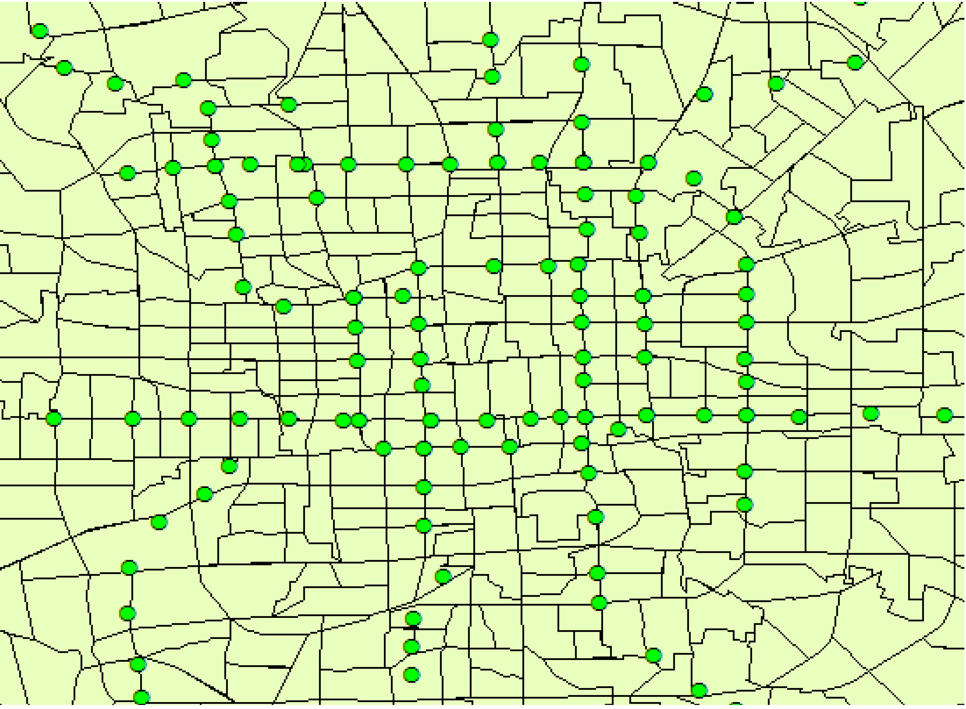
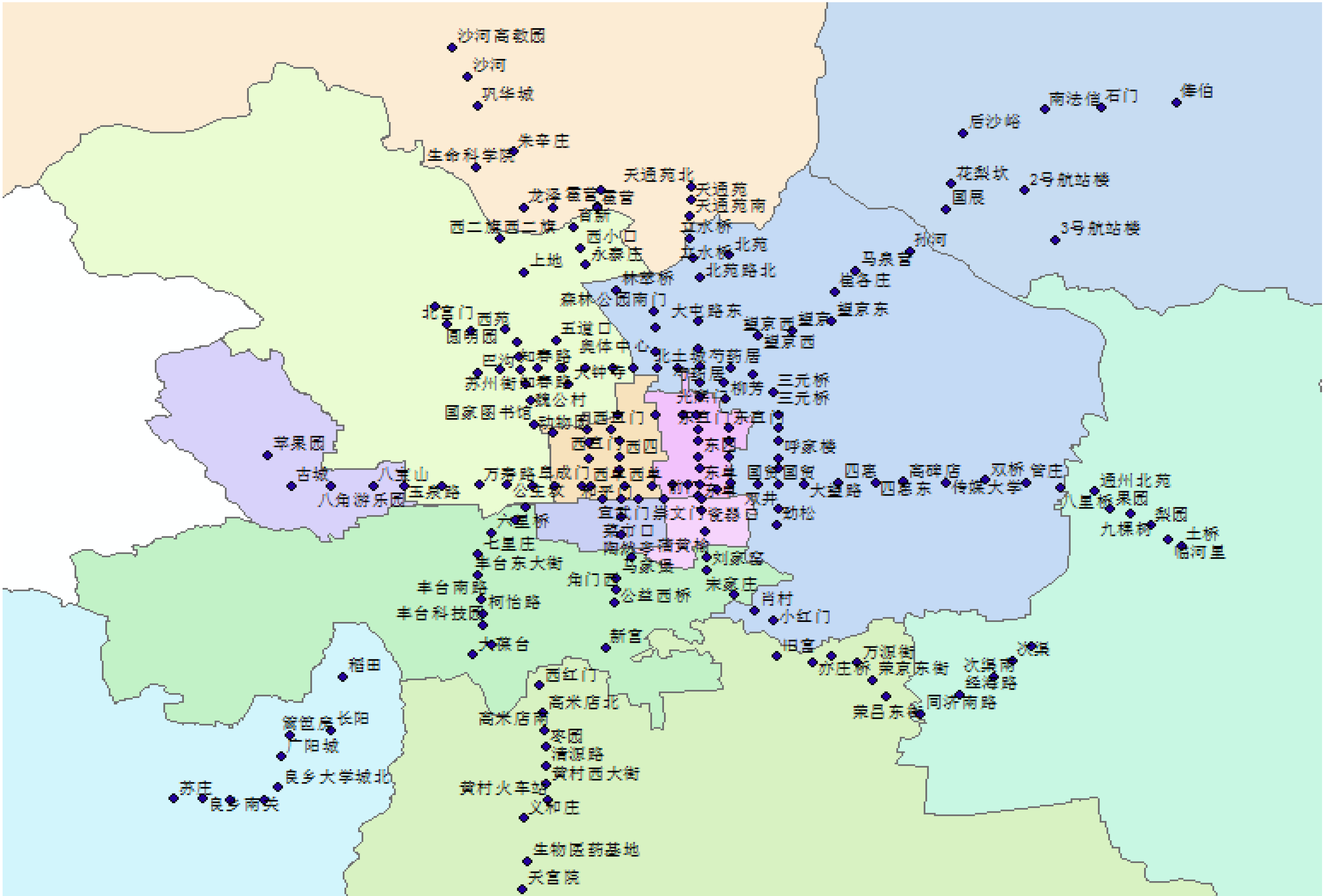
According to the current TAZ delineating result of Beijing, most transit stations are on the boundary of TAZs, as shown in
Figure 1. According to statistics, there are 189 transit stations now in operation (does not include airport line, and transfer stations are only counted once), of which 171 stations are on or nearly on the boundary of TAZs. This accounts for over 90% of all stations. In traditional four-step forecasting, trips are aggregated to the centroid of TAZs, but in urban transit travel, trips are both from and to transit stations. If transit stations are on the boundary of TAZs, there would be a serious reduction of the forecasting accuracy.
Figure 1.
Transit station distribution and current Traffic Analysis Zone (TAZ) delineating.
Figure 1.
Transit station distribution and current Traffic Analysis Zone (TAZ) delineating.
Current TAZ delineating method cannot reflect the relationship between transit stations and TAZs, and is not sensitive enough to the change of factors such as land use and traffic condition around transit station.
2.2. Deficiencies of Catchment Area in Sketch-Level Forecasting
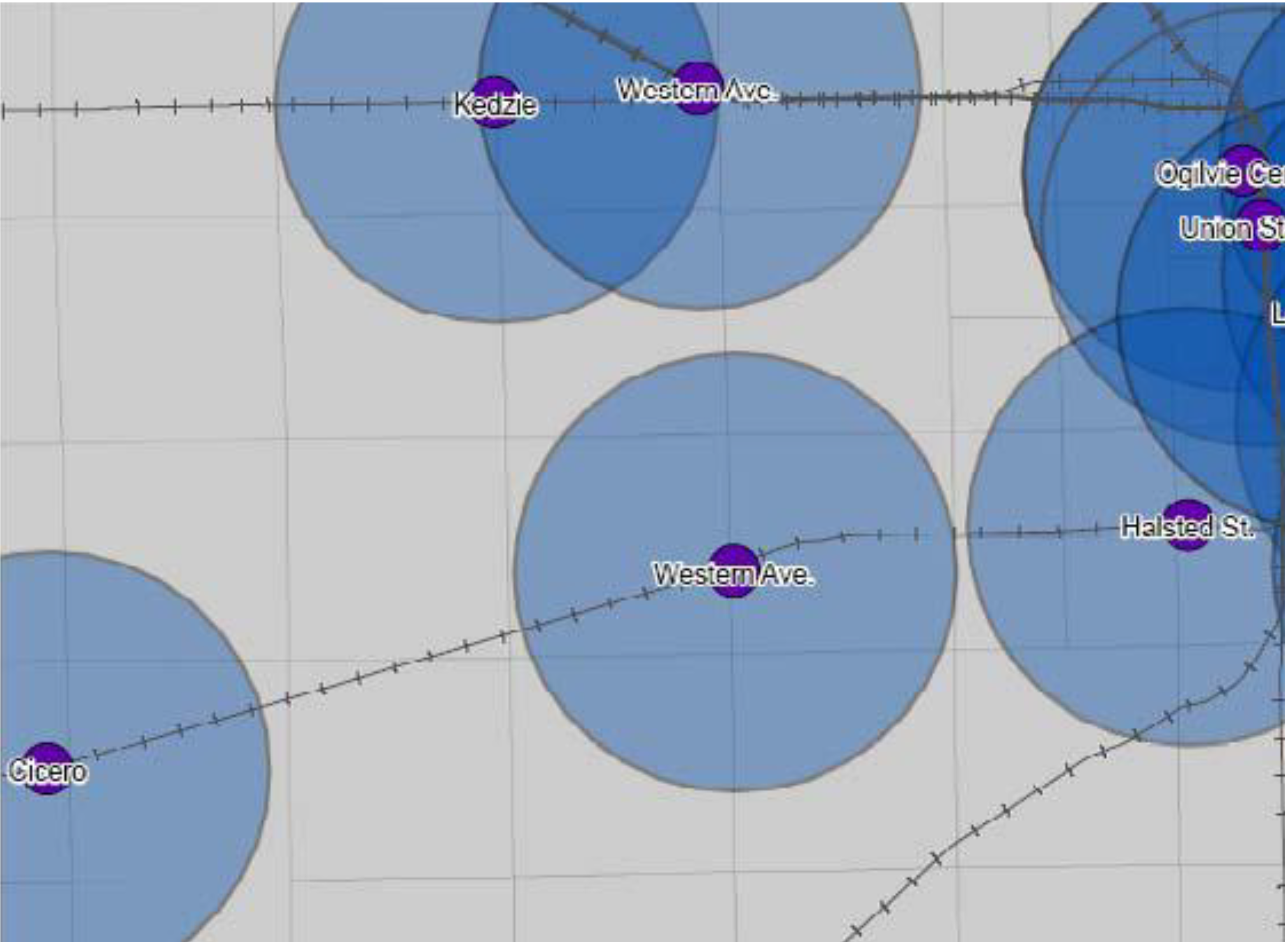
Acting as a “Traffic Analysis Zone”, catchment area has its advantages: it reflects the correlation between transit stations and “TAZs”; it is sensitive to the local changes of land use and traffic conditions around transit station; delineating results would change correspondingly with the change of transit traffic conditions. However, the disadvantages are also obvious: catchment areas are separated from each other and unsystematic, leading to the disability to distribute travel demand city-wide and forecasting the volume of transfer passengers; catchment areas are usually not large enough to cover all travel demands towards the corresponding transit station, as shown in
Figure 2, travel demand from passengers living out of “TAZ” will be ignored. In big cities with concentrated travel demand and serious traffic jams like Beijing, most of the long distance travel would rely on urban transit, and this part of demand cannot be ignored.
On the basis of
Section 2.1 and
Section 2.2, come up with the basic requirement of TTAZ delineating:
- (1)
Each TTAZ should contain one transit station, which is the centroid of the corresponding TTAZ.
- (2)
TTAZs should cover all areas between any two transit stations, and could distribute travel demand city-wide.
Figure 2.
Transit stations catchment area.
Figure 2.
Transit stations catchment area.
3. TTAZ Delineating Method Based on Thiessen Polygon
Considering the requirements of TTAZ delineating, introduce Thiessen polygon from Meteorology into TTAZ delineating. The detailed introduction to Thiessen polygon and instance validation of TTAZ delineating with Beijing urban transit system is as follows.
3.1. Introduction to Thiessen polygon
Thiessen polygon is also called Dirichlet polygon and Voronoi polygon. In 1911, Dutch climatologist A H Thiessen presented a new method to calculate average rainfall based on discrete distributed weather stations: connect all adjacent weather stations into triangles, and draw the perpendicular bisector of each side of these triangles, thus, the perpendicular bisectors around each weather station could form a polygon. Rainfall intensity of one polygon is indicated by the only weather station contained, and the polygon was then called Thiessen polygon [
21]. The features of Thiessen polygon are: Each Thiessen polygon contains one discrete point;Any point in a Thiessen polygon has the closest distance to the corresponding point;Points on the boundary have the equal distance to the two points on both sides.
To delineate TTAZs using Thiessen polygon, the procedures are:
- (1)
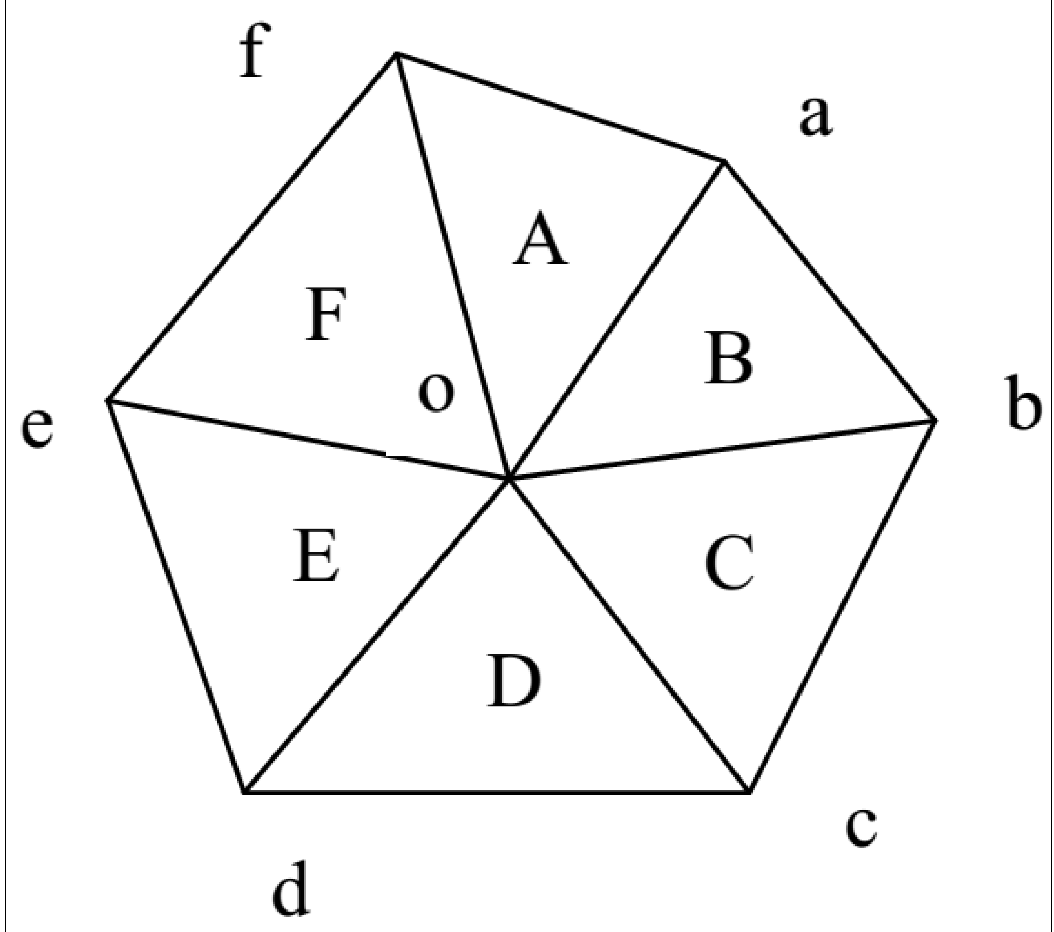
Connect all transit stations into triangles, which is called Delaunay Triangulation network, as
Figure 3 shows. Then, number all the transit stations and triangles, and record which three stations was each triangle composed of.
- (2)
Record the serial number of all adjacent triangles of each transit station.
- (3)
Order the adjacent triangles of each station by clockwise or counterclockwise. Mark one station as
o, find one triangle that contains
o, and mark it as
A. Take another vertex of
A, mark it as
a, and the other one as
f. So the next triangle must have an edge, mark it
F, and the other vertex of triangle
F as
e, so
oe is an edge of the next triangle. Repeat the procedures above until get back to
oa, as
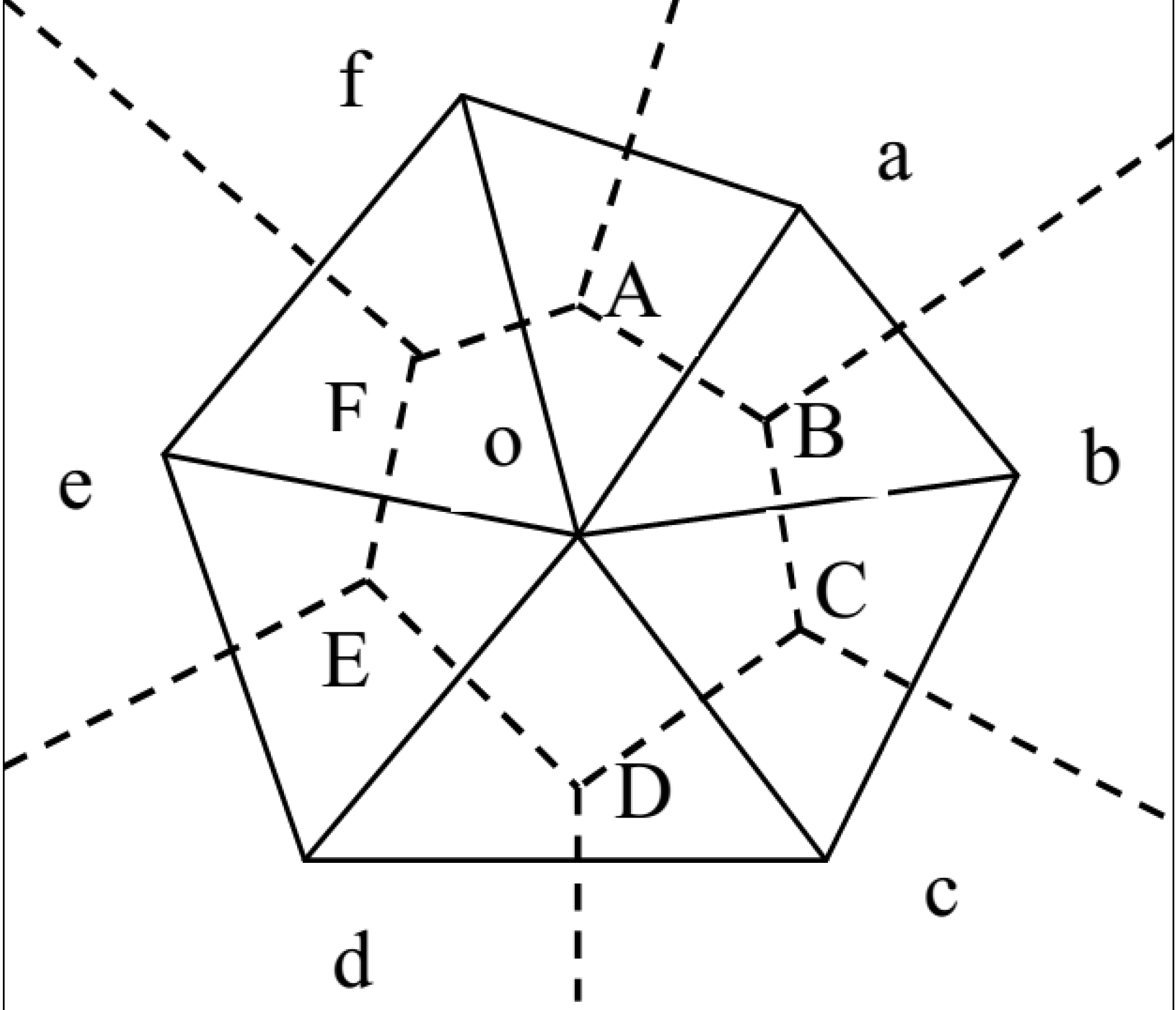
Figure 4 shows, the polygon constituted by dotted line is Thiessen polygon, vertexes of which are the circumcircle centers of each triangle.
- (4)
Calculate the circumcircle of each triangle and record them.
- (5)
According to the adjacent triangles of each station, connect the centers of their circumcircles and get Thiessen polygons. For Thiessen polygons outside of the Delaunay triangulation network, extend the perpendicular bisectors to the figure profile, and forming Thiessen polygons with the figure profile.
Figure 3.
Delaunay triangulation network.
Figure 3.
Delaunay triangulation network.
Figure 4.
Thiessen polygon construction procedures.
Figure 4.
Thiessen polygon construction procedures.
3.2. Beijing TTAZ Delineating
In order to validate the feasibility of Thiessen polygons in TTAZ delineating, take Beijing as an example and carried out TTAZ delineating on the basis of Thiessen polygon using ArcGIS. Delineating procedure is as follows:
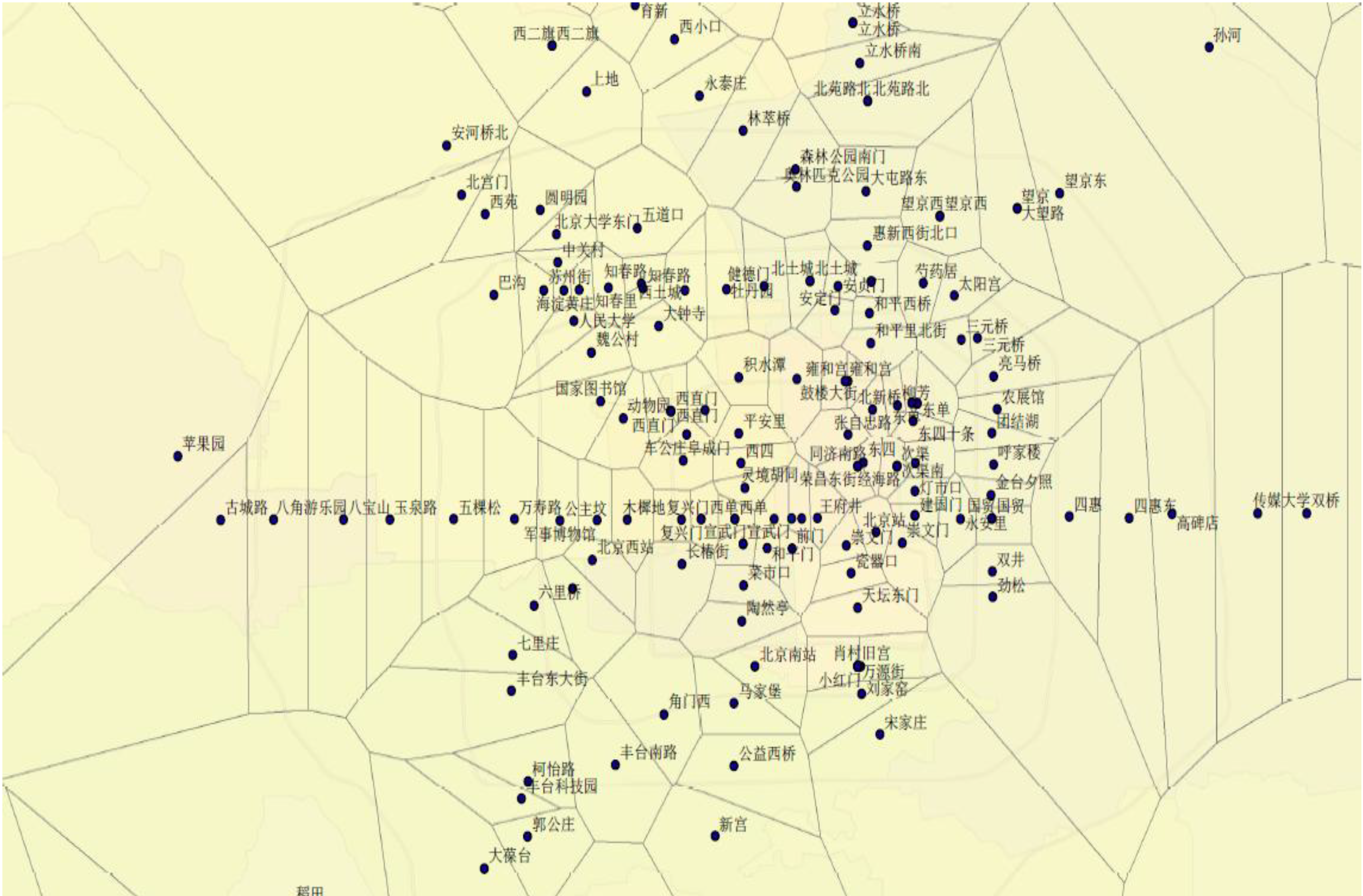
Get the latitude and longitude coordinates of transit stations using handheld GPS logger, and import them into geographic information system to match with the WGS84 (World Geodetic System 1984) coordinate Beijing map, as shown in
Figure 5.
Figure 5.
Transit station coordinates matched with Beijing map.
Figure 5.
Transit station coordinates matched with Beijing map.
Using corresponding tools in ArcTollbox to delineate Transit ridership forecasting Traffic Analysis Zones (TTAZs), and the delineating results is shown in
Figure 6.
TTAZ delineated with Thiessen polygons has the following advantages:
- (1)
Polygon centroid of TTAZ is transit station, the start point and end point of transit trips would be more in line with the actual situation in trip aggregation;
- (2)
The transit travel OD (The passenger volume from Origin to Destination) between TTAZs is easy to get through the analysis of AFC (Automatic Fare Collection) data;
- (3)
TTAZ delineation would change with the change of transit condition, thus reducing the complexity and subjectivity of TTAZ delineating;
- (4)
The connection distance in any part of a TTAZ to the corresponding transit station is relatively clear.
Figure 6.
Beijing TTAZ delineating results.
Figure 6.
Beijing TTAZ delineating results.
3.3. TTAZ Feasibility Validation
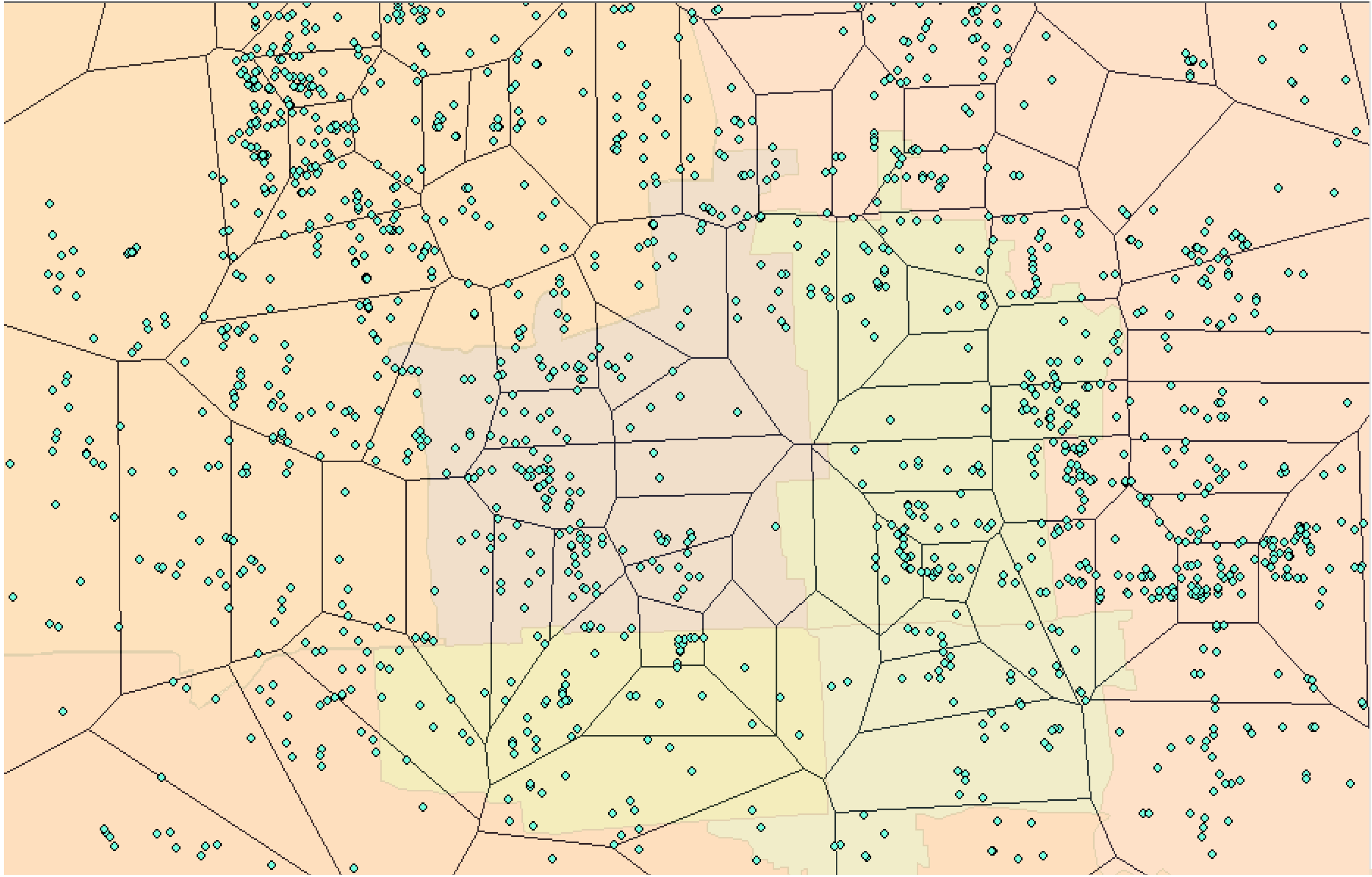
In order to validate the feasibility of TTAZ in transit ridership forecasting, we need to conduct an analysis of the correlation between TTAZ land use features and passenger flow of the corresponding transit station. However, due to data limitations, land use features of TTAZs cannot be described precisely. Therefore, selected 1765 office buildings in Beijing randomly and get their coordinates, import them into Geographic Information System, and conduct a primary spatial analysis, as
Figure 7 shows.
Figure 7.
Distribution of office buildings in TTAZ.
Figure 7.
Distribution of office buildings in TTAZ.
We carried out an overlay analysis with 10 randomly selected TTAZ, get the number of office buildings that fall in each TTAZ. Since office buildings have the closest correlation with work trips, and most of the companies in Beijing start to work at 9:00 am, we investigated the outbound volume of corresponding transit stations during 8:00–9:00 am, and the data obtained is shown in
Table 1.
Table 1.
Office buildings within each TTAZ and outbound volume of corresponding transit stations.
Table 1.
Office buildings within each TTAZ and outbound volume of corresponding transit stations.
| Station Name | Office Building Number | Outbound volume |
|---|
| NongZhanGuan | 3 | 1383 |
| ShuangJing | 11 | 5758 |
| CiQiKou | 12 | 3627 |
| JinTaiXiZhao | 13 | 7920 |
| DaZhongSi | 13 | 4593 |
| ShangDi | 14 | 5919 |
| AnDingMen | 15 | 4246 |
| HuJiaLou | 16 | 6218 |
| MuDanYuan | 23 | 5439 |
| SanYuanQiao | 29 | 10777 |
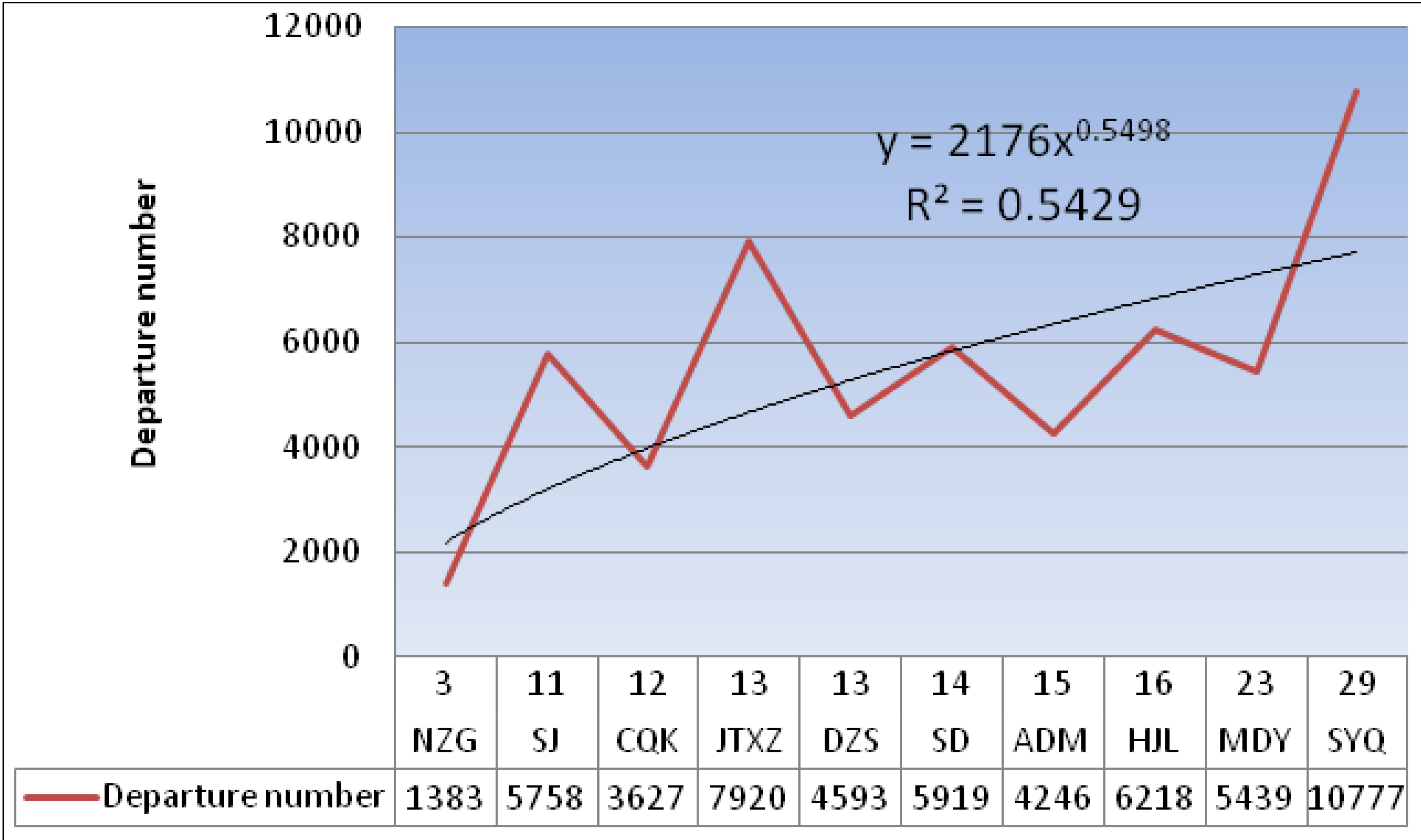
We drew the relationship between office building number and outbound volume, and there is an obvious trend that the outbound volume increases with the increase of office building number, as
Figure 8 shows.
Figure 8.
Regression result of TTAZ proposed by this paper.
Figure 8.
Regression result of TTAZ proposed by this paper.
Conduct a regression analysis of office building number and outbound volume, the regression result is shown in
Table 2.
Table 2.
Regression results of office building number and outbound volume.
Table 2.
Regression results of office building number and outbound volume.
| Functional form | Fit result | Fit goodness |
|---|
| Liner function | y = 518.62x + 2735.6 | R2 = 0.3877
|
| Exponential function | y = 2636.3e0.1161x | R2 = 0.413
|
| Quadratic function | y = 26.375x2 + 228.49x + 3315.8
| R2 = 0.3941
|
| Power function | y = 2176x0.5498 | R2 = 0.5429
|
| Logarithmic function | y = 2172.8ln(x) + 2306.2
| R2 = 0.3988
|
Compare the fit goodness of different functional form, and choose Power function as the relationship model:
where:
R2 = 0.5429, means there is moderately strong relationship between transit station outbound volume and the corresponding TTAZ office building number. Consequently, the TTAZ delineating method proposed in this paper reflects the transit travel characteristic of passengers and has the potential of forecasting the transit ridership more accurately on the basis of taking full account of the passenger influencing factors; it is of further research value. Additionally, the result is obtained under simplified conditions, without considering the influence of office building size, distance to corresponding transit station, and some other factors affecting passenger flow volume such as other types of buildings, feed bus condition, private car ownership, etc. There will be a better fitting result when these factors are added in future research.
4. Conclusions
The TTAZ delineating method proposed in this paper bears a potential for improving the accuracy of current transit ridership forecasting methods. Meanwhile, the TTAZs can also act as catchment areas, which could be used not only for feeder bus arrangement, but also for land use mix development policy making. Mixed land use means the development of different types of buildings within a certain range of the area. Mixed land use could help to shorten the average travel distance of residents’ daily travel between origins and destinations, which will be a significant relief to the urban traffic pressure.
In the future, more detailed building information within TTAZs of Beijing will be studied in order to reveal the correlation between land use characteristics and transit ridership, and thus improve the accuracy of transit ridership forecasting models.
It should be pointed out that the purpose of Transit Traffic Analysis Zone is not to replace the function of traditional TAZ, it can only act as a supplement of traditional TAZ to analyze transit station service. TTAZs cannot be used for the analysis of other modes.
Acknowledgments
This work was financially supported by the National Natural Science Foundation of China (No. 51308017, 51108028), the Beijing Municipal Natural Science Foundation (No. 8122009), Beijing Nova program, the China Scholarship Council, and the Ministry of Industry and Information Technology of People’s Republic of China under the Major Program of national science and technology with No. 2013ZX01045003-002.
Author Contributions
Shuwei Wang had conceived the study and drafted the paper, Lishan Sun and Jian Rong had revised this manuscript, and Zifan Yang had collected the data.
Conflicts of Interest
The authors declare no conflict of interest.
References
- Wang, L.; Liu, X.M.; Ren, F.T. Research on Trip Generation Forecast Method Related to City Land Uses. J. Beijing Polytech. Univ. 2004, 30, 98–101. [Google Scholar]
- Zhang, N.; Ye, X.F.; Liu, J.F. The Impact of Land Use on Demand of Urban Rail Transit. Urban Transp. China 2012, 8, 24–27. [Google Scholar]
- Shi, F.; Jian, W.; Wang, W.; Lu, J. Research on forecast method for traffic creating based on characteristics of land utility. China Eng. J. 2005, 38, 115–118. [Google Scholar]
- Transportation Research Board. Travel Estimation Techniques for Urban Planning. Available online: http://ntl.bts.gov/lib/21000/21500/21563/PB99126724.pdf (accessed on 1 March 2013).
- Cambridge Systematics, Inc.; AECOM Consult. A Recommended Approach to Delineating Traffic Analysis Zones in Florida. Available online: http://www.fsutmsonline.net/images/uploads/reports/FR1_FDOT_Taz_White_Paper_Final.pdf (accessed on 1 March 2013).
- McNally, M.G. The four step model. Available online: http://www.its.uci.edu/its/publications/papers/CASA/UCI-ITS-AS-WP-07-2.pdf (accessed on 1 March 2013).
- Zhao, J.H.; Li, W.Q. Improvement of the Traffic District Partition in Resident Trip Investigation. J. Transp. Eng. Inf. 2009, 7, 110–114. [Google Scholar]
- Ma, C.Q.; Wang, R.; Wang, Y.P.; Yan, B.J.; Chen, K.M. Calculating method of traffic zone radius in city based on inner trip proportion. J. Traffic Transp. Eng. 2007, 7, 68–72. [Google Scholar]
- O’Neill, W.A.; Ramsey, R.D.; Chou, J.C. Analysis of transit service areas using geographic information systems. Available online: http://trid.trb.org/view.aspx?id=371490 (accessed on 1 March 2013).
- Zhao, F.; Chow, L.F.; Li, M.T.; Gan, A.; Ubaka, I. Forecasting transit walk accessibility: Regression model alternative to buffer. Available online: http://www.ltrc.lsu.edu/TRB_82/TRB2003-001007.pdf (accessed on 1 March 2013).
- Murray, A.; Wu, X. Accessibility tradeoffs in public transit planning. J. Geogr. Syst. 2003, 5, 93–107. [Google Scholar] [CrossRef]
- Gutiérrez, J.; García-Palomares, J.C. Distance-measure impacts on the calculation of transport service areas using GIS. Plann. Des. 2008, 35, 480–503. [Google Scholar]
- El-Geneidy, A.M.; Tétreault, P.R.; Surprenant-Legault, J. Pedestrian access to transit: Identifying redundancies and gaps using a variable service area analysis. Available online: http://www.researchgate.net/publication/228389395_Pedestrian_Access_to_Transit_Identifying_Redundancies_and_Gaps_Using_a_Variable_Service_Area_Analysis (accessed on 1 March 2013).
- Alshalalfah, B.; Shalaby, A. Case study: Relationship of walk access distance to transit with service, travel, and personal characteristics. J. Urban Plann. Dev. 2007, 133, 114–118. [Google Scholar] [CrossRef]
- Public Policy and Transit Oriented Development: Six International Case Studies. Available online: http://onlinepubs.trb.org/onlinepubs/tcrp/tcrp_rpt_16-4.pdf (accessed on 1 March 2013).
- Taylor, B.D.; Fink, C.N.Y. The Factors Influencing Transit Ridership: A Review and Analysis of the Ridership Literature. Available online: http://www.uctc.net/papers/681.pdf (accessed on 1 March 2013).
- Miller, H.; Shaw, S. Geographic Information Systems for Transportation: Principles and Applications; Oxford University Press: New York, NY, USA, 2001. [Google Scholar]
- Cervero, R. Alternative approaches to modeling the travel-demand impacts of smart growth. J. Am. Plann. Assoc. 2006, 72, 285–295. [Google Scholar]
- Lane, C.; DiCarlantonio, M.; Usvyat, L. Sketch Models to Forecast Commuter and Light Rail Ridership: Update to TCRP Report 16. Available online: http://www.worldtransitresearch.info/research/392/ (accessed on 1 March 2013).
- Gutiérrez, J.; Cardozo, O.D.; García-Palomares, J.C. Transit ridership forecasting at station level: an approach based on distance-decay weighted regression. J. Transp. Geogr. 2011, 19, 1081–1092. [Google Scholar] [CrossRef]
- Thiessen, A.H. Precipitation averages for large areas. Mon. Weather Rev. 1911, 39, 1082–1084. [Google Scholar]
© 2014 by the authors; licensee MDPI, Basel, Switzerland. This article is an open access article distributed under the terms and conditions of the Creative Commons Attribution license (http://creativecommons.org/licenses/by/3.0/).


