Article

Development of Web-Based RECESS Model for Estimating Baseflow Using SWAT

1
Department of Regional Infrastructure Engineering, Kangwon National University, 1 Kangwondaehak-gil, Chuncheon, Kangwon-do 200-701, Korea
2
Department of Biological and Agricultural Engineering, Texas A & M University, College Station, TX 77843-2117, USA
*
Author to whom correspondence should be addressed.
These authors contributed equally to this work.
Sustainability 2014, 6(4), 2357-2378; https://doi.org/10.3390/su6042357
Submission received: 19 January 2014 / Revised: 4 April 2014 / Accepted: 9 April 2014 / Published: 23 April 2014

Abstract

:
Groundwater has received increasing attention as an important strategic water resource for adaptation to climate change. In this regard, the separation of baseflow from streamflow and the analysis of recession curves make a significant contribution to integrated river basin management. The United States Geological Survey (USGS) RECESS model adopting the master-recession curve (MRC) method can enhance the accuracy with which baseflow may be separated from streamflow, compared to other baseflow-separation schemes that are more limited in their ability to reflect various watershed/aquifer characteristics. The RECESS model has been widely used for the analysis of hydrographs, but the applications using RECESS were only available through Microsoft-Disk Operating System (MS-DOS). Thus, this study aims to develop a web-based RECESS model for easy separation of baseflow from streamflow, with easy applications for ungauged regions. RECESS on the web derived the alpha factor, which is a baseflow recession constant in the Soil Water Assessment Tool (SWAT), and this variable was provided to SWAT as the input. The results showed that the alpha factor estimated from the web-based RECESS model improved the predictions of streamflow and recession. Furthermore, these findings showed that the baseflow characteristics of the ungauged watersheds were influenced by the land use and slope angle of watersheds, as well as by precipitation and streamflow.

1. Introduction

Climate change influences the variability of hydrologic responses (i.e., precipitation amounts and frequencies, groundwater recharge and discharge, evapotranspiration, runoff processes, etc.) across the land surface [1,2]. Many studies have reported the steadily increasing variability of hydrologic responses to have negative impacts on water resources management, such as increased severity and frequency of natural disasters [3,4]. According to the fourth report of the Intergovernmental Panel on Climate Change (IPCC), it seems that climate change will aggravate water stress throughout the world, together with population growth, urbanization and changes in land use [5]. Especially the variability of water availability due to climate change has made it more difficult to manage water resources efficiently at the field scale in regions, such as the Republic of Korea (ROK), where flow-duration coefficients (indicating the rate of runoff) are relatively higher. Thus, available groundwater resources provide a natural means to alleviate the effects of the highly variable availability of water in ROK. Furthermore, climate change has more long-term and extensive impacts on groundwater than direct runoff, because the spatio-temporal variability of direct runoff is strongly affected by precipitation. Therefore, sustainable groundwater management is needed for adaptation to climate change.
One of the highest priorities for sustainable groundwater management is to evaluate and appropriate the share of available groundwater that can be feasibly extracted. For this purpose, we need to estimate accurate amounts of groundwater recharge at the watershed scale. In particular, understanding the characteristics of baseflow could be the first step toward a better estimation of groundwater recharge. Great efforts in baseflow estimation using historical streamflow records are based on several approaches, such as the recession curve displacement (RCD) method [6,7,8,9,10,11,12,13], the curve-fitting method [14,15] and the water-table fluctuation method [16,17,18,19]. Furthermore, the Hydrograph Separation Program (HYSEP) [20], PART [10], RORA [10], BFLOW [11], the Web-GIS-based Hydrograph Analysis Tool [21,22] (WHAT) systems and tracer-based hydrograph separation methods [23,24] have been employed to separate baseflow from streamflow. For example, Kim [25] estimated groundwater recharge using the baseflow-recession curve and a rainfall-runoff model and made a comparison of the results from these two methods. Kim et al. [26] and Bae and Kim [27] estimated baseflow quantity and the groundwater recharge rate using the Natural Resources Conservation Service (NRCS)-Curve Number (CN) method and baseflow separation, respectively. Yang and Chi [28] obtained high correlation coefficients between baseflow rates and groundwater-table elevations in the analysis using WHAT. Among these baseflow separation models, WHAT is the web-based tool that can separate baseflow from direct runoff by using the Local Minimum method, BFLOW filter [29] and Eckhardt filter [30,31]. Eckhardt [28] proposed representative values of baseflow index (BFImax) for various aquifers, but the use of BFImax (i.e., the maximum of the long-term ratio of baseflow to total streamflow) values specific to regional situations is recommended instead. For this reason, a genetic algorithm-based BFImax analyzer was developed for providing the optimal BFImax parameter to obtain local watersheds and aquifer characteristics for the long-term separation of baseflow from streamflow [22]. With antecedent soil moisture, groundwater storage, precipitation rates and amounts, the analysis of the recession curve plays an important role in understanding the baseflow characteristics at the watershed scale. For quantifying baseflow from hydrograph separation, the WHAT system [21,22,28] adopting the BFLOW parameter [11,32] has mainly been used. However, the digital filter [33] is limited in its consideration of hydrologic watershed features, because the digital filter algorithm simply separates low-frequency signatures from the high-frequency signatures through the signal-analysis process.
The United States Geological Survey (USGS) RECESS model [10], one of the most widely used baseflow-separation programs, can perform more accurate baseflow separations compared to HYSEP or BFLOW, by constructing a master-recession curve (MRC) from streamflow. Furthermore, the recession index (K) derived from RECESS, which is the time required for the streamflow recession by one log cycle [10], can be used to identify the recession characteristics of watersheds in many parts of the world. Many watersheds within ROK are usually small and steep, because about 70% of ROK is mountainous. These geological characteristics can contribute to a shortened travel time of flow from one point of a watershed to another. The RECESS model has been suggested for analyzing long-term recession characteristics that had runoff histories [10]. The RECESS model is a long-standing method used to analyze recession in many other studies across the world, but its accessibility should be improved, while its applicability needs to be extended to include other operating systems and not only MS-DOS. One method to improve the applicability is a web-based system, which builds upon the field-scale RECESS model’s advantage for policymakers. Specifically, the web-based HYSEP [34] and WHAT systems [21] were developed and widely applied in various field-scale studies. The RECESS model provides the recession index (K), which can be used to estimate the alpha factor, a parameter also used in the Soil and Water Assessment Tool (SWAT). Therefore, the applicability of RECESS also needs to be extended to web-based systems.
Typically, the RECESS baseflow separation requires observed streamflow data at gauge stations; the SWAT model [35] can simulate land-atmosphere processes (i.e., streamflow, baseflow, etc.) and has been used to predict hydrologic responses at ungauged watersheds. SWAT has an advantage when applied to large-scale ungauged watersheds by adapting auto-calibration tools, such as Parameter Solution (ParaSol) [36], Sources of Uncertainty Global Assessment using Split Samples (SUNGLASSES) [37,38], Shuffled Complex Evolution-University of Arizona (SCE-UA) [36] and SWAT-calibration and uncertainty procedures (CUP) [39]. For example, Park et al. [40] and Lee et al. [41] tested the applicability of SWAT to small watersheds and performed the estimation of runoff curve coefficients, respectively. Furthermore, Lee et al. [42] and Jung et al. [43] suggested parameter regionalization using SWAT at ungauged watersheds. If calibrated by observations of streamflow in a watershed at the gauged downstream, streamflow at the ungauged upstream can be predicted by the SWAT model. Currently, SWAT has adopted several auto-calibration tools for the training of SWAT parameters (e.g., curve number (CN), threshold depth of water in the shallow aquifer required for return flow to occur (GWQMN), baseflow recession factor (ALPHA_BF)). These calibration tools are designed to find the parameter sets satisfying specific given thresholds, from numerous parameter combinations, which may be physically meaningless. For this reason, it is difficult to consider the calibration characteristics of each SWAT parameter with the auto-calibration tools. Among the SWAT parameters, the alpha factor, which is strongly dependent on stream recession, can be distorted by the calibration processes of the various other parameters related to streamflow, including peak flow and low flow. In such cases, it is difficult to obtain accurate streamflow recession during SWAT calibrations. In this regard, recession information from the observed streamflow can contribute to the improvement of streamflow prediction using SWAT for baseflow separation in an ungauged watershed.
Accordingly, the objectives of this study are three-fold (Figure 1): (1) to develop the web-based RECESS model to build up the advantages of the RECESS program; (2) to evaluate the recession in streamflow prediction using SWAT at a gauged watershed; and (3) to estimate baseflow at ungauged watersheds.
Figure 1. Primary objectives of this study. SWAT, Soil and Water Assessment Tool; WHAT, Web-GIS-based Hydrograph Analysis Tool.
Sustainability 06 02357 g001

2. Materials and Method

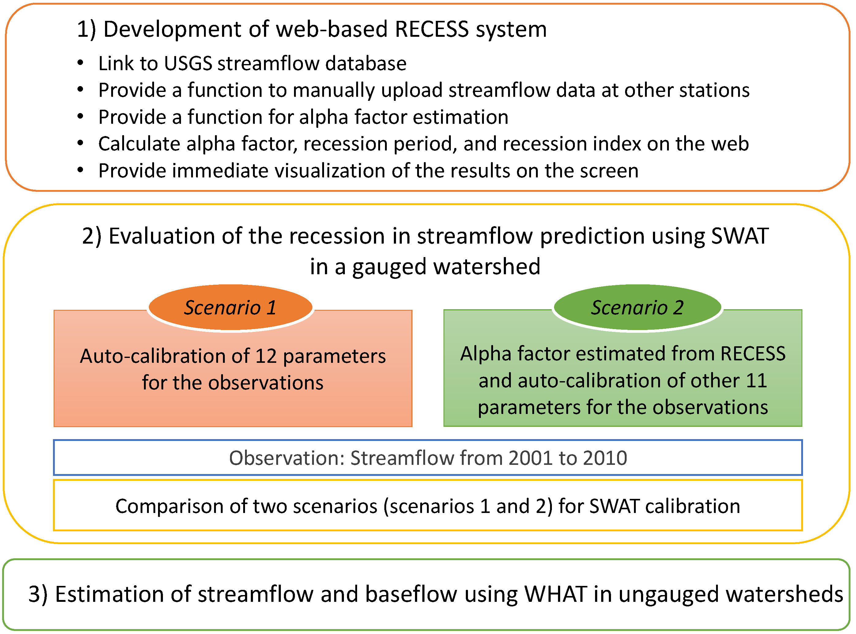
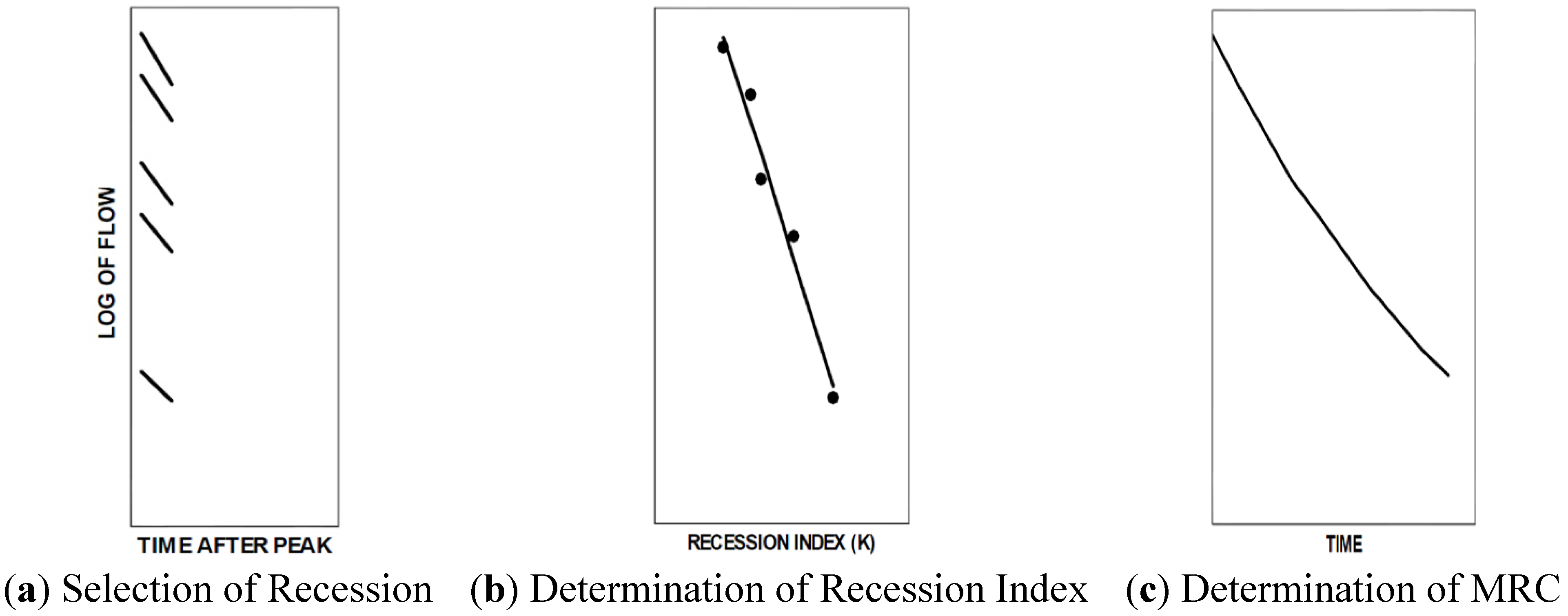
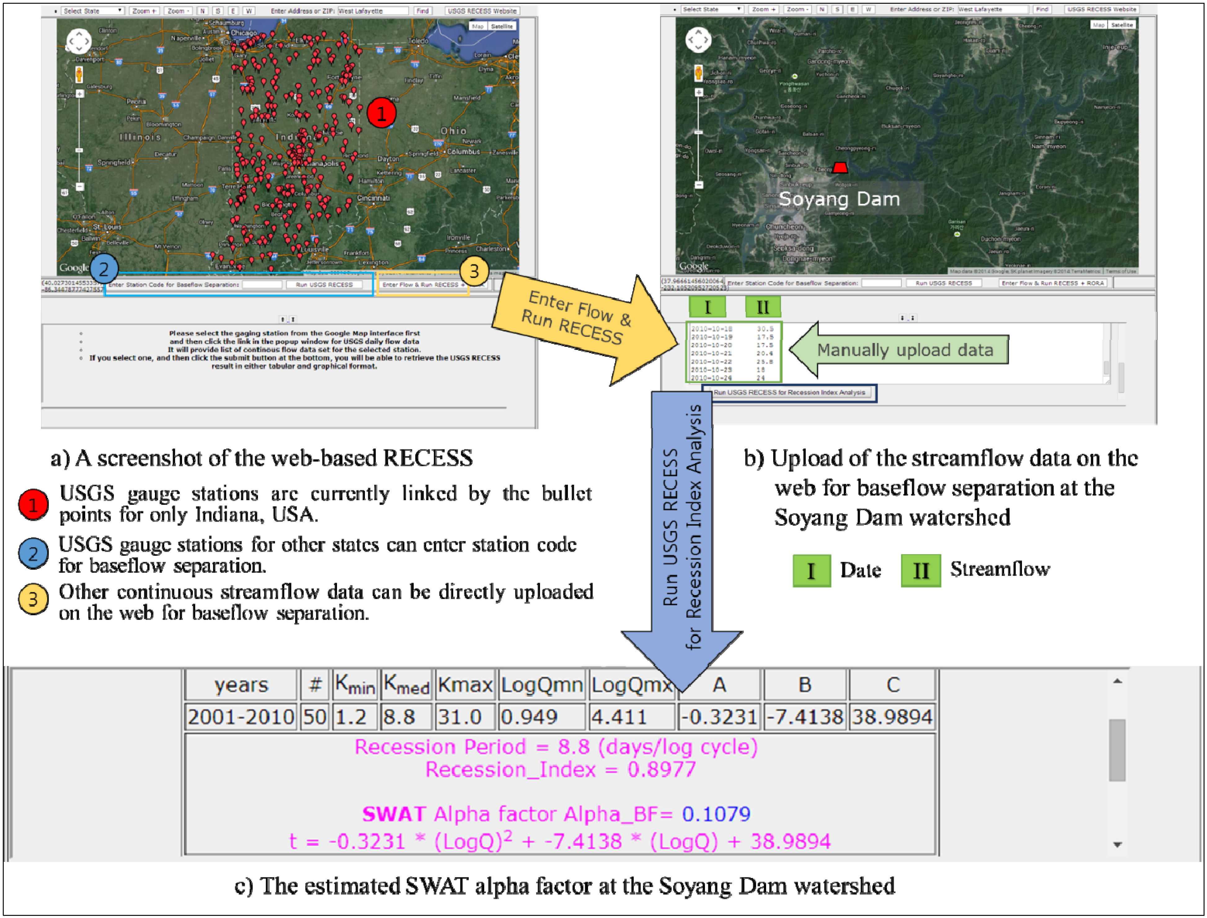
2.1. Development of the Web-Based RECESS Model

The RECESS model was developed by the USGS and has been widely used to analyze recession characteristics using long-term watershed runoff. The original RECESS model on the MS-DOS system consists of several sub-programs. To run the model, users need to make some efforts to repeat the conventional manual input of commands and data. To overcome these inconveniences, we developed a web-based RECESS model to automate these processes through web programming languages, such as Practical Extraction and Report Language (PERL) [44], and Common Gateway Interface (CGI). Furthermore, the web-based interface adopted Google Maps, improving the usability, accessibility and practicability of RECESS. Particularly, the web-based model provides a function to download streamflow data from the USGS National Water Information System (NWIS) website based on Google Maps, allowing for the instantaneous use of actual data. Furthermore, streamflow data can be manually uploaded from other locations through the Internet, and parameters and results estimated from RECESS calculations can be made immediately available through the Internet.
In general, SWAT [35] is a well-validated semi-distributed hydrological model for reproducing streamflow and baseflow based on atmospheric forcings and land-surface information. The SWAT model uses an alpha factor as the baseflow-recession constant in separating baseflow from streamflow. The newly developed web-based RECESS model derives the alpha factor using streamflow data obtained from gauged stations and provides its estimated value to SWAT as an input variable to improve the estimation of baseflow.
In RECESS, the estimated recession index (K) and MRC contribute significantly to the baseflow-separation processes.
As shown in Figure 2, the RECESS model involves three main computation steps: (1) separate the recession from the hydrograph (Figure 2a); (2) estimate K (Figure 2b); and (3) determine the MRC (Figure 2c). Here, the best-fit linear equation for K, which is represented by the dots in Figure 2b, as a function of LogQ based on the recession interval only (Equation 1).
Figure 2. Calculation of the master-recession curve (MRC) [45].
Sustainability 06 02357 g002
t = K1 × LogQ+ K2
where t is time in days, LogQ is the logarithm of the flow and K1 and K2 are regression coefficients. This equation is used to obtain the recession index (K) (days/log cycle), which is the absolute value of K1.
Equation 2 shows how the recession period, T, is calculated when determining the MRC (Figure 2c), which is a polynomial expression of time as a function of LogQ. More detailed information on MRC is available in the study of Rutledge [45].
T = (t − t0) = {A ×(LogQ)2 + B × (LogQ) + C}{t0}
where T is the recession period, t is time from t0 time at peak flow, A, B and C denote the coefficients related to the recession curve and Q is the streamflow.
The web-based RECESS model developed in this study provides the alpha factor to extend the applicability of the RECESS model and increase convenience, while using SWAT-based applications. The alpha factor (α) in the web-based RECESS model may be calculated using Equation 3.
Qt = Q0Kt = Q0e−αt
α = − ln K
where Q0 is discharge at the recession starting point, Qt is discharge at time t and K is the recession index.

2.2. Description of SWAT and SWAT-CUP

SWAT is a semi-distributed hydrological model through which we can run scenarios to investigate the effects of climate or land use, and it has been widely used as a rainfall-runoff model [46,47]. It requires lots of parameters (see Table 1) associated with hydrologic processes (i.e., rainfall-runoff, groundwater recharge/discharge, evapotranspiration) and requires calibration of parameter sets for accurate predictions. For the calibration of SWAT, auto-calibration tools have been developed and/or improved. Recently, to incorporate various calibration modules into SWAT for automating calibration processes or uncertainty analysis, SWAT-calibration and uncertainty programs (SWAT-CUP) [39] was developed. This program includes the sequential uncertainty fitting algorithm (SUFI2) [39], Generalized Likelihood Uncertainty Estimation (GLUE) [48], Parameter Solution (ParaSol) [36], Markov chain Monte Carlo (MCMC) [49] and particle swarm optimization (PSO) calibration [50]. Furthermore, by selecting the appropriate calibration algorithms corresponding to their needs, users can calibrate the SWAT model with observations at multiple outlets within a watershed. Moreover, user can manually adjust the period of observation used for calibration (e.g., the period of recession or flood). In this study, calibration was performed using the SUFI2 algorithm, which has been used to optimize SWAT parameters in many studies [39,51,52].
Typically, streamflow recession information contributes to the accuracy of baseflow estimations, because the natural flow mechanism in the stream can be taken into account by streamflow recession [53]. For example, a stream with a short recession period has a higher variability of seasonal baseflow influence than one with a long recession period. In particular, streamflow is seasonally dominated by direct flow or baseflow. Therefore, streamflow recession information can help to understand the seasonal roles of direct flow and baseflow to a stream for sustainable river management. In this context, the streamflow recession influences baseflow in calibrating rainfall-runoff models. Among the many parameters involved in the SWAT model, the alpha factor is one of the most important parameters, as it is the baseflow-recession coefficient. However, in SWAT calibrations conducted with the numerous parameter sets, the alpha factor can be distorted by various other parameters related to streamflow (i.e., peak and low frequencies), because multiple concurrent processes influence the recession. Considering this, accurate baseflow estimates might prove elusive to SWAT calibrations. Accordingly, uncertainties in streamflow predictions may propagate into the accuracy of baseflow estimations at ungauged watersheds, because baseflow is generally separated from the predicted streamflow derived from rainfall-runoff models. Therefore, streamflow predictions made using SWAT need to reflect the recession appropriately, by considering the alpha factor for accurate baseflow estimations at ungauged watersheds. Thus, we tested the prediction performances of SWAT with alpha factors using two methods: (1) the web-based RECESS and (2) the SWAT-CUP model.
Uncertainties in the calibration and prediction processes of SWAT can be typically represented by several model evaluation statistics [54]. Specifically, the agreement of the calibrated and observed data can be assessed with Nash–Sutcliffe efficiency (NSE) [55], prediction efficiency (Pe) [56], persistence model efficiency (PME) [57], percent bias (PBIAS) [57], daily root-mean square (DRMS) [57], root mean square error (RMSE), the RMSE-observations standard deviation ratio (RSR) [58], the coefficient of determination (R2) and mean square error (MSE). Of these methods, the R2, NSE and PBIAS were used to evaluate the SWAT calibrations applied to this study. The R2 measures the degree of collinearity between observations and simulations (Equation 4).
Sustainability 06 02357 i001
where yobs, i is the i-th observation, ysim, i is the i-th simulation, Yobs is the mean of the observations, Ysim is the mean of the simulations and n is the total number of observations.
The NSE is a normalized statistic that gives the relative magnitude of the residual variance compared to the observed variance [55] and is calculated by using Equation 5:
Sustainability 06 02357 i002
where one NSE value indicates perfect agreement between observations and simulations.
PBIAS describes the average tendency of simulations to be over- or under-estimated compared to observation [57], and it may be calculated by using Equation 6:
Sustainability 06 02357 i003
where a zero PBIAS value indicates perfect agreement between observations and simulations. Positive and negative PBIAS values indicate model bias caused by under- and over-estimations, respectively.

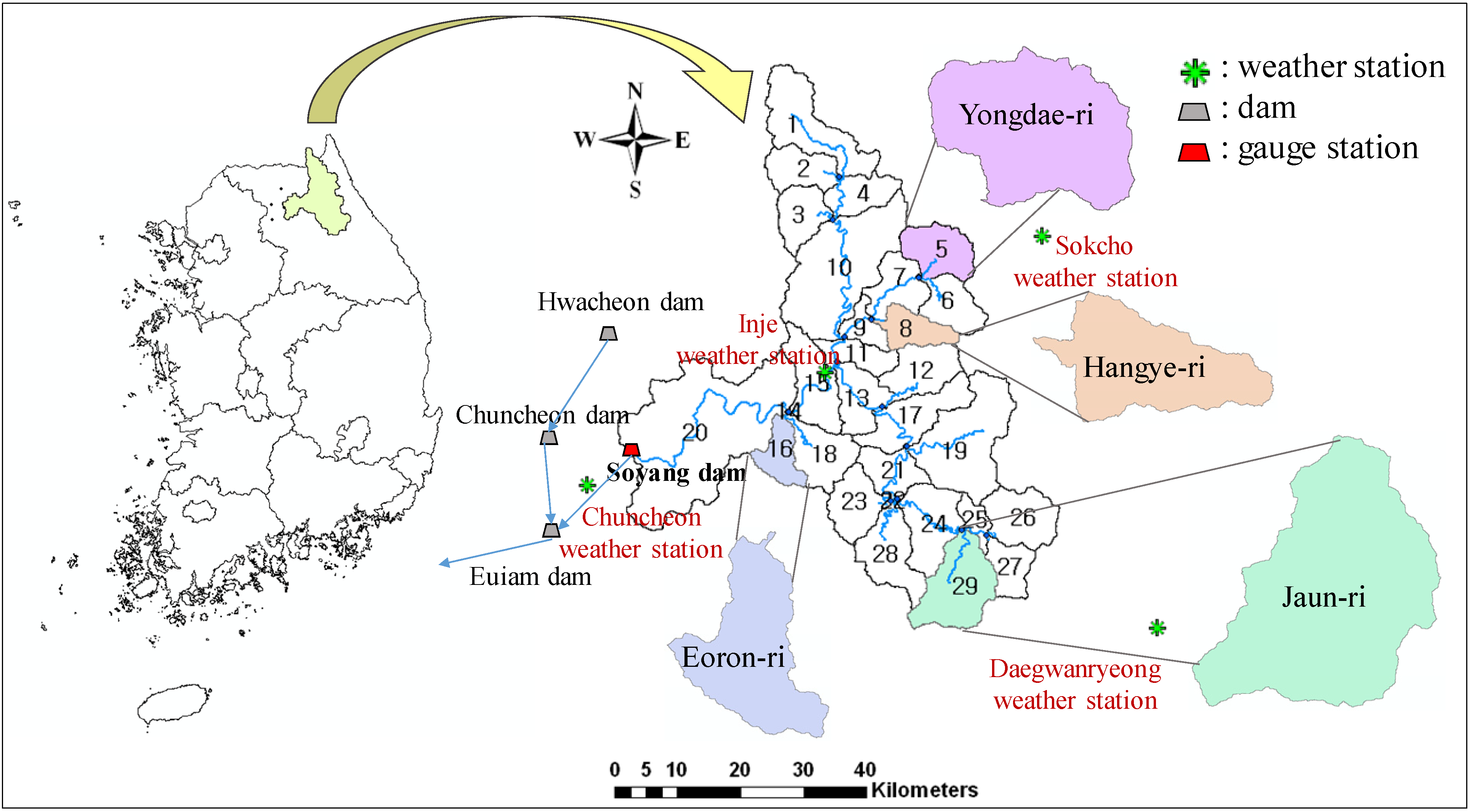
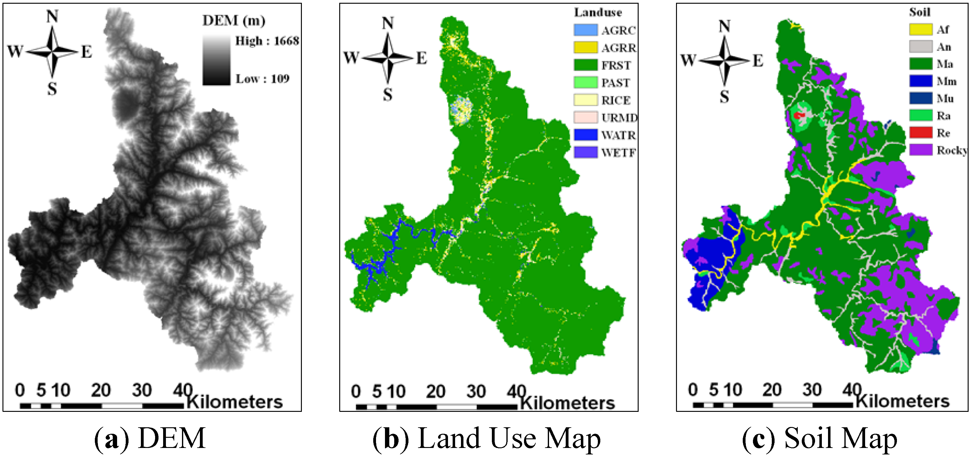
2.3. Descriptions of the Study Area and SWAT Input Data

Since July, 2012, Anabaena, a kind of blue green algae, has bloomed at the Euiam dam in the upstream of North Han River (ROK). The major causes might be abnormally high temperature and decreased and less frequent rainfall compared to historical years [59]. Water quantities and quality and temperature at the Euiam dam are usually affected by water discharge from the Chuncheon and Soyang dams. The Soyang dam is the largest multipurpose dam in ROK for the generation of hydropower, flood control and water supply. Thus, the Soyang dam has a large storage capacity with good water qualities compared to other dams within the Han River basin [60]. For these reasons, the regulation of water discharge from the Soyang dam has become a politically and environmentally sensitive issue, as it represents one of the ways to mitigate algae blooms at the Euiam dam during the dry seasons. Thus, we selected the Soyang dam watershed for testing the newly developed web-based RECESS. The inflow data (flow into the Soyang dam) is retrieved from the Soyang dam gauge station. These inflow data were used to calibrate the SWAT model. Note that the Chuncheon dam watershed was excluded from this study, because the water quantities and quality for this watershed are significantly influenced by regulated discharge from the Hwacheon dam located further upstream.
The Soyang dam watershed is located in the Northeast of ROK, with a total area of about 2694 km2. The watershed boundary length is 386.6 km, and the average elevation is about 650.5 m with an average slope of 40.6% (Figure 3). In addition to these geological specifications, 92% of the entire watershed is covered by forest in that the relatively low streamflow discharge (approximately 3.29 m3/s) during the dry seasons is shown. The Advanced Spaceborne Thermal Emission and Reflection Radiometer (ASTER) Global Digital Elevation Model (GDEM) were used in this study (Figure 4a), and its resolution is 30 m × 30 m. ASTER GDEM is a product of the Ministry of Economy, Trade and Industry (METI), Japan, and the National Aeronautics and Space Administration (NASA), the United Sates (U.S.). Furthermore, the intermediate classified land use map is available from the Water Management Information System (WAMIS), as shown in Figure 4b. Land use at the Soyang dam watershed is composed of 91.8% forest (FRST), 1.7% water (WATR), 0.7% residential-medium density (URMD), 0.4% agricultural land-clos-grown (AGRC), 0.1% wetlands-forested (WETF), 0.5% pasture (PAST), 2.0% rice (RICE) and 2.7% agricultural land-row corps (AGRR), respectively. Furthermore, a reconnaissance soil map provided by the Rural Development Administration was used (Figure 4c). Figure 4c shows a brief descriptions of soil type which are as follows: Af (alluvial soils and river wash, flood plains), An (complex of soils, narrow valleys), Ma (lithosols, siliceous crystalline), Mm (lithosols, micaceous and hard siliceous), Mu (brown forest soils and lithosols, undifferentiated), Ra (red-yellow podzolic soils, siliceous crystalline), Re (lithosols, severely eroded, siliceous) and Rocky (rocky lands).We collected daily atmospheric observations (e.g., precipitation, maximum and minimum temperature, solar radiation, humidity, wind speed) from the four climate gauge stations within the Soyang dam watershed.
Figure 3. Location of the study area. The numbers from 1 to 27 indicate the sub-watersheds within the Soyang dam watershed.
Sustainability 06 02357 g003
Figure 4. Input parameters of the SWAT model within the Soyang dam watershed.
Sustainability 06 02357 g004

2.4. Evaluations of the SWAT Recession Curve Based on the SWAT-CUP and Web-Based RECESS Models

We calibrated the SWAT model using SWAT-CUP with the runoff observed during the entire 15-year period (1996–2010) at the Soyang dam watershed. The observed runoff data for the initial five years were used for a warm up period of the model. Furthermore, we calibrated the model parameters using the inflow observed during the 10-year simulation period (2001–2010) at a Soyang dam gauge station (Figure 3). During the calibration processes, the NSE statistic was used as an objective measure of accuracy [54,55,61]. To allow the 12 model parameters to converge to their optimized values, differences between simulations and observations were minimized during the calibration (Table 1).
Table 1. Initial condition of the parameters for the SWAT-calibration and uncertainty procedures (CUP) auto-calibration. NRCS, Natural Resources Conservation Service.
ParametersDescriptionsVariation MethodsLower
Bound
Upper
Bound
CN2NRCS runoff curve number for moisture Condition IIMultiply by value−0.150.08
ALPHA_BFBaseflow alpha factorReplaced by value0.001.00
GW_DELAYGroundwater delayReplaced by value180.00480.00
GWQMNThreshold depth of water in the shallow aquifer required for return flow to occurReplaced by value05000
GW_REVAPGroundwater “revap” coefficientReplaced by value0.010.14
ESCOSoil evaporation compensation factorReplaced by value0.801.00
CH_N2Manning’s “n” value for the main channelReplace by value0.100.50
CH_K2Effective hydraulic conductivity in main channel alluviumReplace by value−16.0082.00
SOL_AWCAvailable water capacity of the soil layerMultiply by value (%)−0.250.20
SOL_KSaturated hydraulic conductivityMultiply by value (%)−0.940.22
SOL_BDMoist bulk densityMultiply by value (%)−0.040.88
SFTMPSnowfall temperatureReplaced by value−1.296.19

2.5. Estimating Baseflow by Combining SWAT and WHAT at Ungauged Watersheds

After using the observations collected at the gauged watersheds to ensure well-calibrated SWAT parameters, these parameters were used to predict streamflow at each of the ungauged sub-watersheds located within the Soyang dam watershed (Figure 3): Yongdae-ri, Han-gye-ri, Dong-myeon and Jaun-ri. Individual areas of the selected ungauged watersheds are 76.85 km2 for Yongdae-ri, 55.58 km2 for Hangye-ri, 51.51 km2 for Eoron-ri and 131.34 km2 for Jaun-ri, respectively. The resulting streamflow estimates were uploaded to the online WHAT system [62] as input data for baseflow separation.

3. Results and Discussion

3.1. Development of the Web-Based RECESS Model and the Estimation of Alpha Factor

To extend the availability and applicability of the existing RECESS, this study automated user-access and output processes through a web-based interface. Furthermore, by basing the interface on Google Maps (Figure 5a), actual streamflow data at the USGS gauge stations selected by users can be used nearly instantaneously [62]. As shown in Figure 5a, the USGS gauge stations are currently only linked by bullet points for the U.S. state of Indiana. The USGS gauge stations for other states require that a station code be entered for baseflow separation. For countries other than the U.S., the interface provides additional functions that allow users to upload streamflow data directly to the modeling environment, upon which these data can be immediately processed (Figure 5b). Figure 5b shows a screenshot of the web-based RECESS while uploading Soyang dam watershed streamflow data. Furthermore, Figure 5c shows the alpha factor, the K-value (recession index) and recession period for the Soyang dam watershed, calculated by the web-based RECESS model. The estimated alpha factor can then be input into the SWAT model as the Alpha_BF parameter. For the estimation of the alpha factor, we applied our proposed system to the Soyang dam watershed using the inflow data obtained during the 10-year simulation period (2001–2010). As shown in Figure 5c, the web-based RECESS model produced recession period of 8.8 (days/log cycle), recession index (K) of 0.89777, and alpha factor (α) of 0.108 for Soyang dam gauge station.
The estimated alpha factor was 0.108 day−1 for the streamflow observed at Soyang dam gauge station (Figure 5b). In this study, the application of the web-based RECESS model to the Soyang dam watershed requires manual uploading of streamflow data for estimation of the alpha factor, because the web-based RECESS model is currently only linked to USGS gauge stations. However, after clicking the button “Enter Flow & Run RECESS” in Figure 2b, streamflow and drainage area data can be easily uploaded by using the copy/paste functions. The main advantages of the newly developed web-based RECESS model are: (1) to extend the accessibility of the RECESS model through the Internet; and (2) to enhance the efficiency of user-access and output processes related to analyzing and deriving characteristics of streamflow recession. More importantly, the alpha factor obtained by the web-based RECESS model may be used for the determination of streamflow recession in the process of SWAT calibration.
Figure 5. The web-based RECESS model.
Sustainability 06 02357 g005

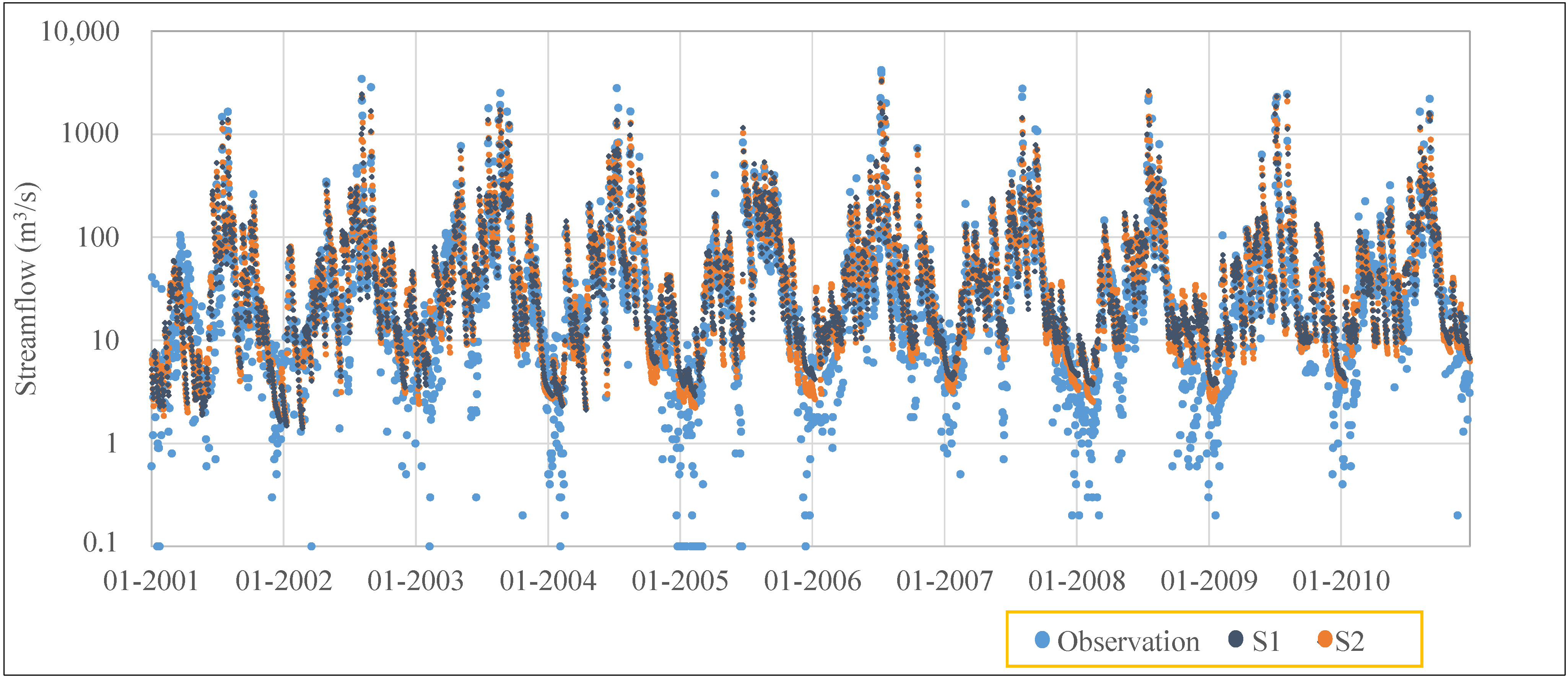
3.2. Impact of the Alpha Factor on the SWAT Calibration Using SWAT-CUP

The SWAT-CUP program was used to calibrate the SWAT model for the 10-year simulation period (2001–2010) in Scenarios I and II, by using daily-observed streamflow. For Scenario II, the alpha factor obtained from the web-based RECESS model was used, which is also the one of the SWAT input. Furthermore, the optimal values of the other 11 parameters were estimated by minimizing the differences between simulated and observed streamflow (indicated by maximal NSE and minimal absolute PBIAS) during the calibration of model parameters, as defined in the SWAT-CUP program. Table 2 presents the results of optimized parameters during the recession processes for Scenarios I and II. The alpha factors estimated for Scenarios I and II were considerably different. That is, the alpha factor for Scenario I (α = 0.663) is considerably higher than Scenario II (α = 0.108). Generally, alpha factors in the range of 0.1–0.3 indicate a slow groundwater recharge response, while alpha factors in the range of 0.9–1.0 indicate a rapid recharge response. The auto-calibration used for Scenario I resulted in SWAT streamflow predictions with much larger alpha factor (α = 0.663) than Scenario II (α = 0.108). Therefore, Scenario I indicates a more rapid groundwater recharge response than Scenario II. However, because the SWAT model is a semi-distributed model and, thus, can be affected by the sub-watershed of a watershed while estimating the alpha factor and the RECESS model estimates a single integrated alpha factor based on a hydrograph at a single outlet of a watershed, the alpha factors obtained from the SWAT model and the RECESS model can be different.
Table 2. Parameters calibrated by SWAT-CUP for Scenarios I and II.
ParametersScenario IScenario II
CN2−0.030−0.070
ALPHA_BF0.6630.108
GW_DELAY212.700232.230
GWQMN4725.0004980.108
GW_REVAP0.118−0.239
ESCO0.9610.915
CH_N20.4930.220
CH_K23.100−60.429
SOL_AWC(1)0.2470.205
SOL_K(1)0.0400.531
SOL_BD(1)0.4190.336
SFTMP−0.4504.451
Figure 6 presents the observed and simulated streamflow results at a logarithmic scale for Scenarios I and II, respectively. In Figure 6, the simulated streamflow shows less fluctuation in the vertical distribution than the observed streamflow, for both Scenarios I and II. From the comparison of Scenarios I and II, it can be seen there seems to be no significant difference between the simulations used for Scenarios I and II, although low-flow was captured slightly better by Scenario II. The SWAT simulations used for Scenarios I and II produced average annual streamflow of 1048.74 mm·year-1 and 980.25 mm·year−1, respectively (Table 3). Considering the observed average annual streamflow of 874.04 mm·year−1, these quantitative results clearly show that Scenario II produced more accurate simulations of streamflow. However, both Scenarios I and II overestimated streamflow compared to the observed streamflow. Calibrations resulted in high NSE values of 0.818 and 0.822, for Scenarios I and II, respectively. Moreover, PBIAS values were −20.0% and −12.2%, for Scenarios I and II. According to the SWAT performance rating shown in Table 4 [54], the acceptable NSE and PBIAS criteria ensuring satisfactory calibration are NSE ≥ 0.5 and PBIAS ≤ ±25%, respectively. Based on these criteria, the SWAT performance ratings for Scenario I are “very good” according to NSE (0.818) and “satisfactory” according to PBIAS (−20.0%). For Scenario II, the SWAT performance ratings are “very good” according to NSE (0.822) and “good” according to PBIAS (−12.2%). Here, the PBIAS statistic indicates that the simulated streamflows were overestimated compared to observed streamflows and that Scenario II overestimated these streamflows less severely. However, uncertainties that have propagated into streamflow predictions may still exist, because other model parameters might affect the model outputs (e.g., the GWQMN and CH_K2 parameters in Table 2).
Table 3. Result for the observed and simulated streamflows based on SWAT-CUP. NSE, Nash–Sutcliffe efficiency; PBIAS, percent bias.
ScenariosAAS (mm·year−1)R2NSEPBIAS (%)
I1048.740.820.818−20.0
II980.250.830.822−12.2
Observation874.04---
Figure 6. Results from the SWAT calibrations for the scenarios.
Sustainability 06 02357 g006
Table 4. Reported performance ratings for the NSE and PBIAS statistics [54].
MethodValuePerformance RatingModeling PhaseReference
NSENSE ≥ 0.65Very goodCalibration and validationSaleh et al. [63]
0.54 < NSE ≤ 0.65AdequateCalibration and validationSaleh et al. [63]
NSE > 0.50SatisfactoryCalibration and validationSanthi et al. [56]
PBIASPBIAS < ±10%Very goodCalibration and validationVan Liew et al. [64]
±10% < PBIAS < ±15%GoodCalibration and validationVan Liew et al. [64]
±15% < PBIAS < ±25%SatisfactoryCalibration and validationVan Liew et al. [64]
Note: AAS is the average of annual streamflow per unit area.
In this study, there is a significant difference between the PBIAS statistics for Scenarios I and II. However, the NSE statistics are similar for both scenarios. This is possibly because an integrated alpha factor was applied to a semi-distributed model at a single outlet of a watershed in Scenario II. Consequently, the SWAT-CUP program would estimate a higher alpha factor for Scenario I due to sub-basin contributions. In particular, the dominant topographic characteristic of the Soyang dam watershed (i.e., steeper up- than down-stream) can be a source of uncertainty propagating into the alpha factor estimated in the SWAT simulations used for Scenario II. Moreover, although PBIAS was higher for Scenario II, this result is likely not solely attributable to the alpha factor, because other SWAT parameters also play important roles in streamflow simulations. Especially GWQMN and CH_K2 (Table 1) contribute significantly to streamflow, as well as to baseflow, because groundwater recharge only occurs when the aquifer level reaches a threshold value of GWQMN (Table 1), while high values of CH_K2 (Table 1) lead to quick displacement of water from the streambed to the subsurface of a stream or river [65,66]. That these influences should be considered is confirmed by Table 2, which shows high variation in the GWQMN and CH_K2 parameters for both scenarios (Table 2).
Figure 7 shows the observed- and simulated streamflow recessions for Scenarios I and II. Simulated recessions were in better agreement with the observed recessions for Scenario II. That is, the simulations of recessions were performed more accurately for Scenario II, for both high and low streamflows (Figure 7). It seems that the auto-calibration scheme for Scenario I has a lack of spatially distributed discharge observations and inadequate and/or unphysical initial parameter values. Figure 7 shows that the recession simulations were in better agreement with the observed recessions for Scenario II (with a low alpha factor: α = 0.108), compared to Scenario I (with a high alpha factor: α = 0.663). Thus, our findings show that if calibrated for recession periods with a fixed alpha factor, streamflow recession was more accurately predicted by the SWAT model. These findings indicates that the SWAT model will be useful for the planning of sustainable groundwater management.
Figure 7. Observed and simulated streamflow recessions for Scenarios I and II, indicated by blue triangles, green dots and red diamonds, respectively; with streamflow (m3·s−1) on the y-axis and time on the x-axis (day).
Sustainability 06 02357 g007

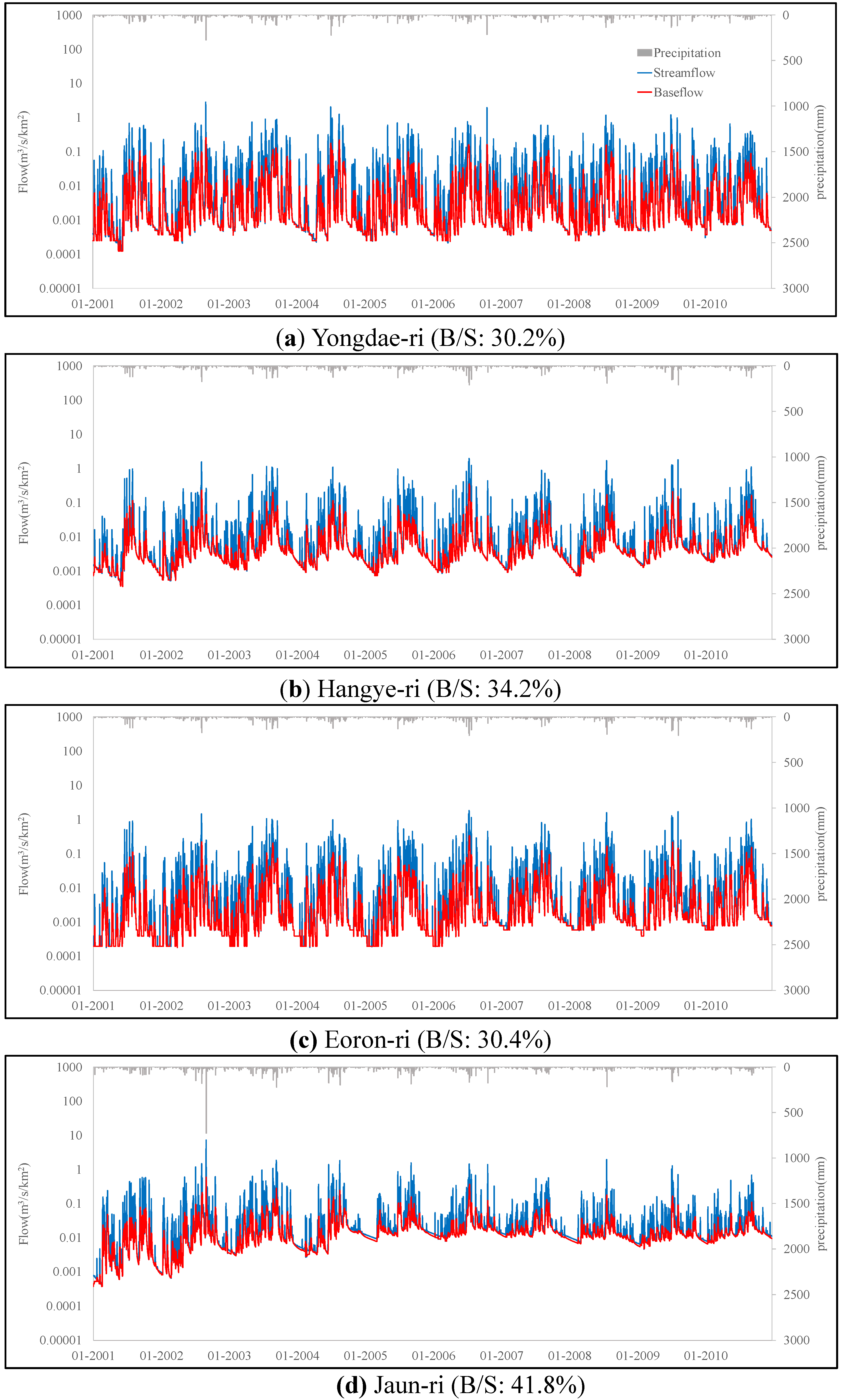
3.3. The Estimation of Baseflow at Ungauged Watersheds

For the baseflow separations, we used the web-based RECESS derived alpha factor of 0.108 to predict the daily streamflow at the ungauged watersheds using SWAT (Figure 8). The frequencies and intensities of atmospheric forcings collected at multiple gauged weather stations were spatially and temporally variable, and baseflow estimates thus showed different trends for individual ungauged watersheds (Table 5). The average annual precipitation amounts (P in Table 5) for Yongdae-ri, Hangye-ri, Eoron-ri and Jaun-ri were 1355.3 mm·year−1, 1376.4 mm·year−1, 1363.1 mm·year−1 and 1838.1 mm·year−1, respectively. Based on the daily streamflow predicted by SWAT, the average annual streamflows (S in Table 5) for Yongdae-ri, Han-gye-ri, Eoron-ri and Jaun-ri were estimated to be 1021.0 mm·year−1, 904.9 mm·year−1, 920.1 mm·year−1 and 1443.1 mm·year−1. Then, these predicted daily streamflows were used as input to the WHAT system for estimation of the baseflow at the ungauged watersheds. The baseflow estimates (B in Table 5) for the four ungauged watersheds range in 280.0 mm·year−1 (minimum, Eoron-ri) to 602.8 mm/year (maximum, Jaun-ri). High ratios of streamflow to precipitation (S/P in Table 5) were found for Jaun-ri and Yongdea-ri, because these watersheds have lower evapotranspiration (ET in Table 5). The ratios of baseflow to average annual precipitation (B/P in Table 5) for Yongdae-ri, Hangye-ri, Eoron-ri and Jaun-ri were 22.8%, 22.5%, 20.5% and 32.8%, respectively. The annual precipitation, streamflow and baseflow were highest in Jaun-ri, which has a wider area and a milder slope than the other watersheds. Furthermore, Yongdae-ri and Eoron-ri have lower ratios of baseflow to streamflow (B/S in Table 5 and Figure 8) than Hagye-ri and Jaun-ri. Figure 8 shows that as B/S becomes higher, the fluctuation in temporal baseflow distribution becomes lower, indicating a dependency. A comparison of Yongdae-ri and Eoron-ri shows that these two ungauged watersheds have large differences in streamflow, baseflow, streamflow per precipitation and baseflow per precipitation, although similar in precipitation. Youngae-ri has greater forest area, less evapotranspiration, a steeper slope and is less urbanized than Eoron-ri. These findings might suggest that the baseflow component is affected not only by precipitation, evapotranspiration and average streamflow, but also by topographical characteristics and land use (Table 5).
Figure 8. Total streamflow and baseflow at log-scale in the ungauged watersheds: (a) Yongdae-ri; (b) Hangye-ri; (c) Eoron-ri; (d) Jaun-ri.
Sustainability 06 02357 g008
Table 5. Watershed characteristics and predicted hydrological responses for individual ungauged watersheds. URMD, residential-medium density; FRST, forest; AGRR, agricultural land-row corps.
WatershedArea (km2)Mean slope (%)Land useP (mm·year−1)ET (mm·year−1)S (mm·year−1)B (mm·year−1)S/P (%)B/P (%)B/S (%)
URMD (%)FRST (%)RICE (%)AGRR (%)Others (%)
Yongdae-ri80.4741.700.8695.501.161.970.511355.3182.11021.0308.575.322.830.2
Hangye-ri54.9350.140.1498.320.810.510.221376.4205.1904.9309.865.722.534.2
Eoron-ri51.5138.511.9590.572.713.930.841363.1200.7920.1280.067.520.530.4
Jaun-ri134.4336.340.9896.631.051.160.181838.1140.81443.1602.878.532.841.8
Notes: P, precipitation; ET, evapotranspiration; S, streamflow; B, baseflow.

4. Conclusions

Groundwater is an important water resource to build up the capacity to adapt to climate change, and scientific information on groundwater characteristics can be used to implement sustainable river management. To promote the capacity of the RECESS program to analyze groundwater characteristics in practice, the web-based RECESS model was developed in this study. Like other gauge stations that provide climatic and hydrologic data, this model can provide information on the alpha factor (α). This study evaluated the alpha factor obtained from the web-based RECESS model as an input, not as a parameter in SWAT applications. To this purpose, the alpha factor derived from the web-based RECESS model was applied to the SWAT model for the separation of baseflow from streamflow. Specifically, we assessed the impacts of streamflow recession on the baseflow characteristics by treating the alpha factor derived from the web-based RECESS model as an input to the SWAT model.
The main conclusions obtained from this study can be summarized as follows.
  • The web-based RECESS model and SWAT-CUP produced alpha factors of 0.108 and 0.663, respectively. These alpha factors were estimated by using two different methods, which was reflected by the considerable differences between them, by the influences on accuracy with which streamflow could be predicted. This might indicate that SWAT-CUP has a limited ability to correctly simulate the characteristics of streamflow recession due to the weighted auto-calibration on the entire streamflow, insufficient observation and (consequently) the lack of a spatially representative distribution of streamflow data.
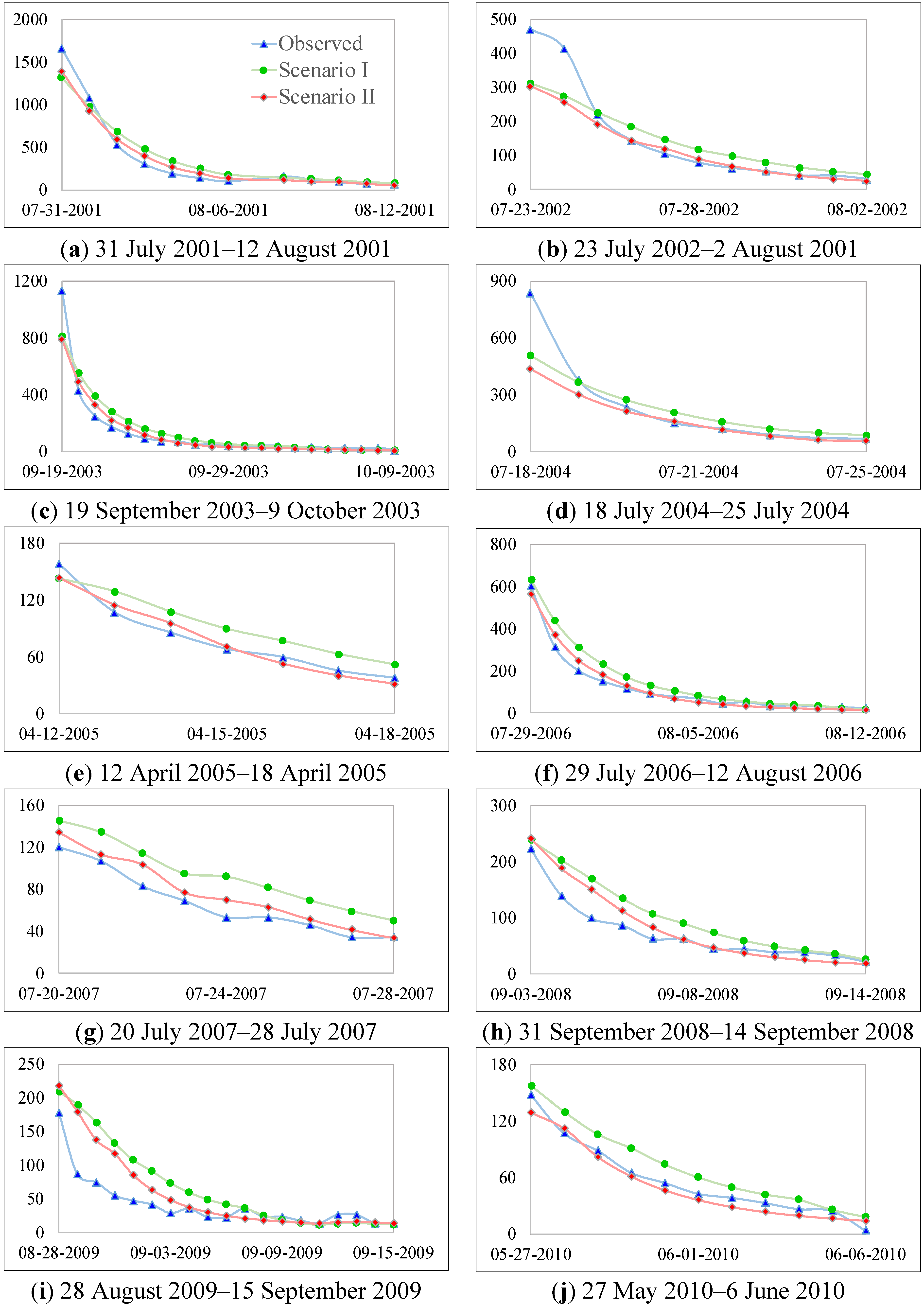
  • The alpha factor obtained from the web-based RECESS model was applied to the calibration of SWAT for streamflow recession periods. As a result, the web-based RECESS model produced good calibration results (NSE: 0.82; PBIAS: −12.2%). The application of the web-based RECESS alpha factor to the SWAT calibrations for streamflow recession periods (Scenario II) resulted in better predictions of streamflow recession (Figure 7). Comparing the individual simulations using Scenarios I and II, Scenario II predicted the recession of low flow more accurately than Scenario II. Based on these findings, this study revealed a significant effect of recession on baseflow. This conclusion is consistent with previous studies that have found the recession to play a major role in baseflow separation [67,68]. However, for better calibration, spatially distributed alpha factors and other parameters associated with groundwater that could affect SWAT simulations should be considered.
  • Initially, it was expected that baseflow would be mainly affected by rainfall and streamflow. However, our findings showed different results compared to those expected (see Section 3.3). For two watersheds that were different in terms of land use, soil texture and topography, similar precipitations produced significant differences in baseflow.
  • This study showed that the ratio of baseflow to streamflow (B/S) affected the temporal baseflow distribution in ungauged watersheds. As B/S is higher, the fluctuation of the temporal baseflow distribution becomes lower.
Based on these findings, the application of the web-based RECESS alpha factor to auto-calibrations for the estimation of recession periods could improve streamflow prediction. Furthermore, the web-based RECESS model can provide easy access to recession information (alpha factor), contribute to extending the applicability of the original RECESS model, help increase its accessibility and increase the convenience with which hydrological modeling may be performed. We expect that the web-based RECESS model will be useful in the identification of the roles of streamflow and baseflow in integrated river basin management and sustainable watershed development.

Acknowledgments

This research was supported by the Geo-Advanced Innovative Action (GAIA) Project (No. RE201402074, Surface Soil Resources Inventory & Integration: SSORII Research Group) in Republic of Korea. I thank Kyong Jae Lim for supporting this research. I also appreciate the editor and other anonymous reviewers for their valuable suggestions.

Author Contributions

Younghun Jung and Yongchul Shin suggested/designed the research theme and methods and wrote the paper. Gwanjae Lee conducted the computer simulations and data analysis. All authors discussed the structure and comment on the manuscript at all stages.

Conflicts of Interest

The authors declare no conflict of interest.

References and Notes

  1. Stocker, T.F.; Raible, C.C. Climate change: Water cycle shifts gear. Nature 2005, 434, 830–833. [Google Scholar] [CrossRef]
  2. Hansena, J.; Sato, M.; Ruedy, R. Perception of climate change. Proc. Natl. Acad. Sci. USA 2012, 109, E2415–E2423. [Google Scholar] [CrossRef]
  3. Piao, S.L.; Ciais, P.; Huang, Y.; Shen, Z.H.; Peng, S.S.; Li, J.S.; Zhou, L.P.; Liu, H.Y.; Ma, Y.C.; Ding, Y.H.; et al. The impacts of climate change on water resources and agriculture in China. Nature 2010, 467, 43–51. [Google Scholar] [CrossRef]
  4. Middelkoop, H.; Daamen, K.; Gellens, D.; Grabs, W.; Kwadijk, J.C.; Lang, H.; Wilke, K. Impact of climate change on hydrological regimes and water resources management in the Rhine basin. Clim. Change 2001, 49, 105–128. [Google Scholar] [CrossRef]
  5. IPCC (Intergovernmental Panel on Climate Change). Climate Change 2007: Synthesis Report. Available online: https://www.ipcc.ch/pdf/assessment-report/ar4/syr/ar4_syr.pdf (accessed on 14 April 2014).
  6. Meyboom, P. Estimating ground-water recharge from stream hydrographs. J. Geophys. Res. 1961, 66, 1203–1214. [Google Scholar] [CrossRef]
  7. Barnes, B.S. The structure of discharge-recession curves. Transactions, Ame. Geophys. Union 1939, 20, 721–725. [Google Scholar]
  8. Bevans, H.E. Estimating stream-aquifer interactions in coal areas in eastern Kansas by using streamflow records. Available online: http://pubs.usgs.gov/wsp/wsp2290/pdf/wsp_2290.pdf (accessed on 14 April 2014).
  9. Hoos, A.B. Recharge rates and aquifer characteristics for selected drainage basins in middle and east Tennessee. Available online: http://pubs.usgs.gov/wri/wri90-4015/pdf/wrir_90-4015.pdf (accessed on 14 April 2014).
  10. Rutledge, A. Computer programs for describing the recession of ground-water discharge and for estimating mean ground-water recharge and discharge from streamflow records: Update. Available online: http://pubs.usgs.gov/wri/wri984148/pdf/wri98-4148.pdf (accessed on 14 April 2014).
  11. Arnold, J.G.; Allen, P.M. Validation of automated methods for estimating baseflow and groundwater recharge from stream flow records. J. Am. Water Resour. Assoc. 1999, 35, 411–424. [Google Scholar] [CrossRef]
  12. Zhu, R.R.; Zheng, H.X.; Liu, C.M. Estimation of groundwater residence time and recession rate in watershed of the Loess Plateau. J. Geog. Sci. 2010, 20, 273–282. [Google Scholar] [CrossRef]
  13. Huang, Y.P.; Kung, W.J.; Lee, C.H. Estimating aquifer transmissivity in a basin based on stream hydrograph records using an analytical approach. Environ. Earth Sci. 2011, 63, 461–468. [Google Scholar] [CrossRef]
  14. Pettyjohn, W.A.; Henning, R. Preliminary estimate of ground-water recharge rates, related streamflow and water quality in Ohio. Available online: https://www.google.com.hk/url?sa=t&rct=j&q=&esrc=s&source=web&cd=1&ved=0CCwQFjAA&url=https%3A%2F%2Fkb.osu.edu%2Fdspace%2Fbitstream%2F1811%2F36354%2F1%2FOH_WRC_552.pdf&ei=scFMU7P8D47fsASSrYKQDA&usg=AFQjCNFnX0bAO90NZ_rCe9hRvbKLQKCCgQ&bvm=bv.64764171,d.cWc&cad=rjt (accessed on 14 April 2014).
  15. Linsley, R.K.; Kohler, M.A.; Paulhus, J.L. Hydrology for Engineers, 3rd ed.; McGraw-Hill: New York, NY, USA, 1982; p. 508. [Google Scholar]
  16. Theis, C.V. Amount of ground-water recharge in the southern high plains. Trans. Am. Geophys. Union 1937, 18, 564–568. [Google Scholar] [CrossRef]
  17. Sophocleous, M.A. Combining the soil water balance and water level fluctuation methods to estimate natural groundwater recharge: practical aspects. J. Hydrol. 1991, 124, 229–241. [Google Scholar] [CrossRef]
  18. Winter, T.C.; Mallory, S.E.; Allen, T.R.; Rosenberry, D.O. The use of principal component analysis for interpreting groundwater hydrographs. Groundwater 2000, 38, 234–246. [Google Scholar] [CrossRef]
  19. Moon, S.K.; Woo, N.C.; Lee, K.S. Statistical analysis of hydrographs and water-table fluctuation to estimate groundwater recharge. J. Hydrol. 2004, 292, 198–209. [Google Scholar] [CrossRef]
  20. Sloto, R.A.; Crouse, M.Y. HYSEP: A computer program for streamflow hydrograph separation and analysis. Available online: http://water.usgs.gov/software/HYSEP/code/doc/hysep.pdf (accessed on 14 April 2014).
  21. Lim, K.J.; Engel, B.A.; Tang, Z.; Choi, J.; Kim, K.; Muthukrishnan, S.; Tripathy, D. Automated web gis based hydrograph analysis tool, WHAT1. J. Am. Water Resour. Assoc. 2005, 41, 1407–1416. [Google Scholar] [CrossRef]
  22. Lim, K.J.; Park, Y.S.; Kim, J.G.; Shin, Y.C.; Kim, N.W.; Kim, S.J.; Jeon, J.H.; Bernard, A.E. Development of genetic algorithm-based optimization module in WHAT system for hydrograph analysis and model application. Comput. Geosci. 2010, 36, 936–944. [Google Scholar] [CrossRef]
  23. Hoeg, S.; Uhlenbrook, S.; Leibundgut, C. Hydrograph separation in a mountainous catchment—Combining hydrochemical and isotopic tracers. Hydrol. Processes 2000, 14, 1199–1216. [Google Scholar] [CrossRef]
  24. Ladouche, B.; Probst, A.; Viville, D.; Idir, S.; Baqué, D.; Loubet, M.; Probst, J.; Bariac, T. Hydrograph separation using isotopic, chemical and hydrological approaches (Strengbach Catchment, France). J. Hydrol. 2001, 242, 255–274. [Google Scholar] [CrossRef]
  25. Kim, N.W.; Chungm, I.M.; Won, Y.S. Method of Estimationg Groundwater Recharge with Spatial-Temporal Variability. J. Am. Water Resour. Assoc. 2005, 38, 517–526. [Google Scholar]
  26. Kim, H.W.; Sin, Y.J.; Choi, J.H.; Kang, H.W.; Ryu, J.C.; Lim, K.J. Estimation of CN-based Infiltration and Baseflow for Effective Watershed Management. J. Korean Soc. Water Qual. 2011, 27, 405–412. (In Korean) [Google Scholar]
  27. Bae, S.K.; Kim, Y.H. Estimation of Groundwater Recharge Rate Using the NRCS-CN and the Baseflow Separation Methods. J. Environ. Sci. 2006, 15, 253–260. (In Korean) [Google Scholar]
  28. Yang, J.S.; Chi, D.K. Correlation Analysis between Groundwater Level and Baseflow in the Geum River Watershed, Calculated using the WHAT System. J. Eng. Geol. 2011, 21, 107–116. [Google Scholar]
  29. Lyne, B.; Hollick, M. Stochastic time-variable rainfall runoff modelling. In Hydrology and Water Resources Symposium, Proceedings. National Committee onHydrology and Water Resources of the Institution of Engineers, Perth, Australia, 10–12 September 1979.
  30. Eckhardt, K. How to Construct Recursive Digital Filters for Baseflow Separation. Hydrol. Processes 2005, 19, 507–515. [Google Scholar] [CrossRef]
  31. Collinschonn, W.; Fan, F.M. Defining parameters for Eckhardt’s digital baseflow filter. Hydrol. Processes 2012, 27, 2614–2622. [Google Scholar] [CrossRef]
  32. Eckhardt, K. A comparison of baseflow indices, which were calculated with seven different baseflow separation methods. J. Hydrol. 2008, 352, 168–173. [Google Scholar] [CrossRef]
  33. Chapman, T.G.; Maxwell, A. Baseflow Separation—Comparison of numerical methods with tracer experiments. Available online: http://search.informit.com.au/documentSummary;dn=360361071346753;res=IELENG (accessed on 14 April 2014).
  34. Jang, W.S.; Park, Y.S.; Kim, J.G.; Engel, B.; Lim, K.J. Development of Google Map-based USGS HYSEP and Application. In Proceedings of the Korea Water Resources Association Conference, Yongpyong, Korea, 22–23 May 2009; pp. 1417–1421. (In Korean)
  35. Arnold, J.G.; Srubuvasan, R.; Muttiah, R.S.; Wiliams, J.R. Large area hydrologic modeling and assessment Part I: Model Development. J. Am. Water Resour. Assoc. 1998, 34, 73–89. [Google Scholar] [CrossRef]
  36. Van Griensven, A.; Meixner, T. Methods to quantify and identify the sources of uncertainty for river basin water quality models. Water Sci. Technol. 2006, 53, 51–59. [Google Scholar] [CrossRef]
  37. Muleta, M.K.; Nicklow, J.W. Sensitivity and uncertainty analysis coupled with automatic calibration for a distributed watershed model. J. Hydrol. 2005, 306, 127–145. [Google Scholar] [CrossRef]
  38. Van Griensven, A.; Meixner, T.; Srinivasan, R.; Grunwald, S. Fit-for-Purpose analysis of uncertainty using split-sampling evaluations. Hydrol. Sci. J. 2008, 53, 1090–1103. [Google Scholar] [CrossRef]
  39. Abbaspour, K.C.; Yang, J.; Maximov, I.; Siber, R.; Bogner, K.; Mieleitner, J.; Zobrist, J.; Srinivasan, R. Modelling hydrology and water quality in the pre-alpine/alpine Thur watershed using SWAT. J. Hydrol. 2007, 333, 413–430. [Google Scholar] [CrossRef]
  40. Park, S.C.; Cho, D.J.; Roh, K.B.; Jin, Y.H. Applicability analysis of SWAT model for a small basin. In Proceedings of the Korea Water Resources Association Conference, Gyeongju, Korea, 22–23 May 2008; pp. 2042–2045. (In Korean)
  41. Lee, J.W.; Kim, N.W.; Lee, J.W.; Seo, B.H. Estimation of runoff curve number for ungaged watershed using SWAT model. J. Korean Soc. Agri. Eng. 2009, 51, 11–16. (In Korean) [Google Scholar]
  42. Lee, J.S.; Kim, S.J.; Kim, D.G.; Kang, N.R.; Kim, H.S. Estimation of hydraulic coefficients in an ungaged basin using SWAT model. J. Korean Wetlands Soc. 2011, 13, 319–327. (In Korean) [Google Scholar]
  43. Jung, Y.H.; Jung, C.G.; Jung, S.W.; Park, J.Y.; Kim, S.J. Estimation of upstream ungauged watershed streamflow using downstream discharge data. J. Korean Soc. Agri. Eng. 2012, 54, 169–176. (In Korean) [Google Scholar]
  44. Wall, L. PERL: Practical Extraction and Report Language. Available online: http://www-cgi.cs.cmu.edu/cgi-bin/perl-man (accessed on 14 April 2014).
  45. Rutledge, A.T. Program user guide for RECESS. Available online: http://water.usgs.gov/ogw/recess/UserManualRECESS.pdf (accessed on 14 April 2014).
  46. Jeong, J.; Kannan, N.; Arnold, J.; Glick, R.; Gosselink, L.; Srinivasan, R. Development and integration of sub-hourly rainfall-runoff modeling capability within a watershed model. Water Resour. Manag. 2010, 24, 4505–4527. [Google Scholar] [CrossRef]
  47. Ryu, J.C.; Cho, J.; Kim, I.J.; Mun, Y.; Moon, J.P.; Kim, N.W.; Kim, S.J.; Kong, D.S.; Lim, K.J. Enhancement of SWAT-REMM to Simulate Reduction of Total Nitrogen with Riparian Buffer. Trans. ASABE 2011, 54, 1791–1798. [Google Scholar] [CrossRef]
  48. Beven, K.; Binley, A. The future of distributed models: Model calibration and uncertainty prediction. Hydrol. Processes 1992, 6, 279–298. [Google Scholar] [CrossRef]
  49. Kuczera, G.; Parent, E.; Monte, C. Assessment of parameter uncertainty in conceptual catchment models: The Metropolis algorithm. J. Hydrol. 1998, 211, 69–85. [Google Scholar] [CrossRef]
  50. Eberhart, R.; Kennedy, J. A new optimizer using particle swarm theory. Available online: http://www.ppgia.pucpr.br/~alceu/mestrado/aula3/PSO_2.pdf (accessed on 14 April 2014).
  51. Rostamian, R.; Jaleh, A.; Afyuni, M.; Mousavi, S.F.; Heidarpour, M.; Jalalian, A.; Abbaspour, K.C. Application of a SWAT model for estimating runoff and sediment in two mountainous basins in central Iran. Hydrol. Sci. J. 2008, 53, 977–988. [Google Scholar] [CrossRef]
  52. Ryu, J.C.; Kang, H.W.; Choi, J.W.; Kong, D.S.; Gum, D.H.; Jang, C.H.; Lim, K.J. Application of SWAT-CUP for Streamflow Auto-calibration at Soyang-gang Dam Watershed. J. Korean Soc. Water Environ. 2012, 28, 347–358. (In Korean) [Google Scholar]
  53. Tallaksen, L.M. A review of baseflow recession analysis. J. Hydrol. 1995, 165, 349–370. [Google Scholar] [CrossRef]
  54. Moriasi, D.; Arnold, J.; van Liew, M.; Bingner, R.; Harmel, R.; Veith, T. Model Evaluation Guidelines for Systematic Quantification of Accuracy in Watershed Simulations. Trans. ASABE 2007, 50, 885–900. [Google Scholar] [CrossRef]
  55. Nash, J.; Sutcliffe, J. River Flow Forecasting through Conceptual Models Part I—A Discussion of Principles. J. Hydrol. 1970, 10, 282–290. [Google Scholar] [CrossRef]
  56. Santhi, C.; Arnold, J.J.R.; Williams, W.A.; Dugas, R.S.; Hauck, L.M. Validation of the SWAT model on a large river basin with point and nonpoint sources. J. Am. Water Resour. Assoc. 2001, 37, 1169–1188. [Google Scholar]
  57. Gupta, H.V.; Sorooshian, S.; Yapo, P.O. Status of Automatic Calibration for Hydrologic Models: Comparison with Multilevel Expert Calibration. J. Hydrol. Eng. 1999, 4, 135–143. [Google Scholar] [CrossRef]
  58. Chu, T.; Shirmohammadi, A. Evaluation of the SWAT Model’s Hydrology Component in the Piedmont Physiographic Region of Maryland. Trans. ASABE 2004, 47, 1057–1073. [Google Scholar] [CrossRef]
  59. Ministry Of Environment of Korea. Strengthening Measures of Drinking-Water treatment systems about the Algae Occurrence in Paldang Water Source Protection Area. Available online: http://www.korea.kr/archive/expDocView.do?docId=32397 (accessed on 14 April 2014). (In Korean)
  60. Park, S.W. A Modeling Study of Hydrodynamic and Temperature Distribution in the Lake Euiam. Master’s Thesis, Ewha Womans University, Seoul, Korea, Janary 2012. [Google Scholar]
  61. McCuen, R.H.; Knight, Z.; Cutter, A.G. Evaluation of the Nash-Sutcliffe Efficiency Index. J. Hydrol. Eng. 2006, 11, 597–602. [Google Scholar] [CrossRef]
  62. The Web-GIS-based Hydrograph Analysis Tool. Available online: http://www.envsys.co.kr/~what/ (accessed on 14 April 2014).
  63. Saleh, A.; Arnold, J.; Gassman, P.W.A.; Hauck, L.; Rosenthal, W.; Williams, J.; McFarland, A. Application of SWAT for the Upper North Bosque River Watershed. Trans. ASAE 2000, 43, 1077–1087. [Google Scholar] [CrossRef]
  64. Van Liew, M.W.; Veith, T.L.; Bosch, D.D.; Arnold, J.G. Suitability of SWAT for the Conservation Effects Assessment Project: Comparison on USDA Agricultural Research Service Watersheds. J. Hydrol. Eng. 2007, 12, 173–189. [Google Scholar] [CrossRef]
  65. Veith, T.L.; van Liew, M.W.; Bosch, D.D.; Arnold, J.G. Parameter Sensitivity and Uncertainty in SWAT: A Comparison Across Five USDA-ARS Watersheds. Trans. ASABE 2010, 53, 1477–1485. [Google Scholar] [CrossRef]
  66. Kannan, N.; White, S.; Worrall, F.; Whelan, M. Sensitivity Analysis and Identification of the Best Evapotranspiration and Runoff Options for Hydrological Modelling in SWAT-2000. J. Hydrol. 2007, 332, 456–466. [Google Scholar] [CrossRef]
  67. Wittenberg, H.; Sivapalan, M. Watershed Groundwater Balance Estimation Using Streamflow Recession Analysis and Baseflow Separation. J. Hydrol. 1999, 219, 20–33. [Google Scholar] [CrossRef]
  68. Nathan, R.; McMahon, T. Evaluation of Automated Techniques for Base Flow and Recession Analyses. Water Resour. Res. 1990, 26, 1465–1473. [Google Scholar]

