Article

Analysis of Two Models for Evaluating the Energy Performance of Different Buildings

by
Luca Evangelisti
,
Gabriele Battista
*,
Claudia Guattari
,
Carmine Basilicata
and
Roberto De Lieto Vollaro
Department of Engineering, University of Roma TRE, via Vito Volterra 62, Rome 00146, Italy
*
Author to whom correspondence should be addressed.
Sustainability 2014, 6(8), 5311-5321; https://doi.org/10.3390/su6085311
Submission received: 5 June 2014 / Revised: 4 August 2014 / Accepted: 5 August 2014 / Published: 14 August 2014

Abstract

:
Nowadays it is possible to employ several software packages to evaluate building’s energy performance, each of them based on a different calculation code, with different boundary conditions in terms of environmental temperature, solar radiation, wind velocity and relative humidity. In this contribution, a comparison between two calculation codes, taking into account different types of buildings, has been carried out. In particular, a semi-stationary calculation code and a dynamic one have been employed to determine energy demands of three different building’s types: an old building, a house and a flat. Analyzing semi-stationary conditions (consequently simplified environmental conditions), a software which applies the UNI TS 11300 standard has been considered. This standard defines the procedures for the national implementation of the UNI EN ISO 13790. Furthermore, in order to consider the environmental conditions variation, a well-known dynamic software has been used.

1. Introduction

Buildings’ energy performance issues have recently become strongly critical for the scientific community: the importance of these topics comes from the need to reduce fuels consumptions and pollutants emissions. In Europe, 80% of carbon emissions comes from urban areas: buildings, industries and transports are a set of elements that greatly contributes to increase pollution in the old continent [1]. A building is a highly complex energy system because it is characterized by the interaction with the surrounding. Therefore, introducing rigorous tools for the energy analysis should be promoted [2]. Plant size depends on buildings performance [3] and on its capability to maintain internal comfort conditions for humans. Nowadays, in order to evaluate construction’s performance, it is possible to employ many software packages characterized by the implementation of different calculation approaches. Over the past 50 years, many building energy codes have been developed. The core tools in the building energy field are the whole-building energy simulation programs, which provide users with key building performance indicators, such as energy use and demand, temperature, humidity, and costs. A number of comparative surveys of energy codes has been published [4]. In the last years, energy diagnosis was a very important issue treated by several international studies [5,6,7,8,9]. In particular, in Italy the European Directive has been applied through the Decree n.192 and recently through the Decree n.63. In Italy, these analyses are based on the UNI TS 11300 standard [10]. These standards require an energy analysis made under semi-stationary conditions, simulating the building energy demand through average values of environmental temperatures, solar radiation and wind velocity. For that reason, this kind of investigation shows the characteristics connected to the stationary features of climatic phenomena, as shown in many studies [11,12,13,14]. Consequently, in order to provide a more detailed analysis, it is possible to use a more complex calculation tool, represented by a dynamic software that allows us to analyze the effects of climatic variations over the time. This choice can lead to a more precise and complete energy demand estimation compared to the steady-state approach, which is commercially available and widely used for energy analysis. Furthermore, the dynamic approach takes into account dynamic properties of the structures and allows us to achieve an accurate modeling process that reflects the real building geometry [15]. The dynamic approach demonstrates high effectiveness and reliability to investigate the influence of external walls thermal inertia properties on the energy performance of buildings [16].
The proposed study wants to point out numerical differences arising from the use of a semi-stationary and a dynamic calculation code applied to different building types, such as a historical building, a house and a flat. The differences of these three different kinds of architectures are related not only to structural characteristics (possible contacts with the ground or gaps around the building) but also take into account the inertial structure properties on annual energy demand variations. It will be seen in the following that the results obtained by the two tools lead to discrepancies of different amount in the energy demand estimation of the three types of buildings.

2. Methodology

As mentioned, the UNI TS 11300 standard, which defines the procedures for the national implementation of the UNI EN ISO 13790 [17], is based on a simplified procedure for the calculation of building energy performance. This procedure relies on a semi-stationary approach that consists in environmental physical simplifications, characterized by monthly average values of several factors, such as environmental temperatures, solar radiation values, wind velocity and relative humidity. The typical daily variables fluctuation is reduced to a single value that can be considered constant throughout the month. Moreover, the inertial behavior of a building is related to two utilization factors. The equations used to calculate the annual energy demand are:
QH ,nd = (QH ,tr + QH ,ve) − ηH ,gn(Qint + Qsol)
QC ,nd = (Qint + Qsol) − ηC ,Is(QC ,tr + QC ,ve)
where, QH ,nd and QC ,nd represent the heating and cooling energy demands, QH ,tr and QC ,tr represent the thermal dispersions through opaque and transparent surfaces for heating and cooling requirements respectively, QH ,ve and QC ,ve represent the ventilation losses, Qint represents the internal gains and Qsol represents the solar gains. The utilization factor of thermal contributions is ηH ,gn and the utilization factor of thermal dispersion is ηC ,Is. We can see that in the equations a term that represents the thermal energy stored by the building’s masses is not explicitly mentioned. The accumulation of heat and its release are taken into account through the coefficients ηH ,gn and ηC ,Is. Considering heating demand, the ratio between heat gain and loss called γH, is defined as follows:
Sustainability 06 05311 i001
where Qgn represents the sum of Qint and Qsol; QH ,ht represents the sum of QH ,tr and QH ,ve. In the standard the utilization factor ηH ,gn is defined as:
Sustainability 06 05311 i002
Sustainability 06 05311 i003
where a is a numerical parameter depending on the time constant τ.
Sustainability 06 05311 i004
Sustainability 06 05311 i005
C is the internal heat capacity of building, H is the building total heat loss coefficient related to transmission and ventilation heat losses. In Equation (7), a0 is a numerical parameter and τ0 is a reference time constant. For the cooling season ηC ,Is is defined in a similar fashion.
The simplified equations above do not accurately describe the inertial behavior of a building, that is represented by the wall’s thermal storage, both in winter and summer, with a subsequent energy demand reduction. This is a physical phenomenon which is independent on the methodology adopted and it should be always taken into account for the buildings energy performance analysis.

2.1. Building Types

The buildings taken into account in this study are placed in the center of Italy.
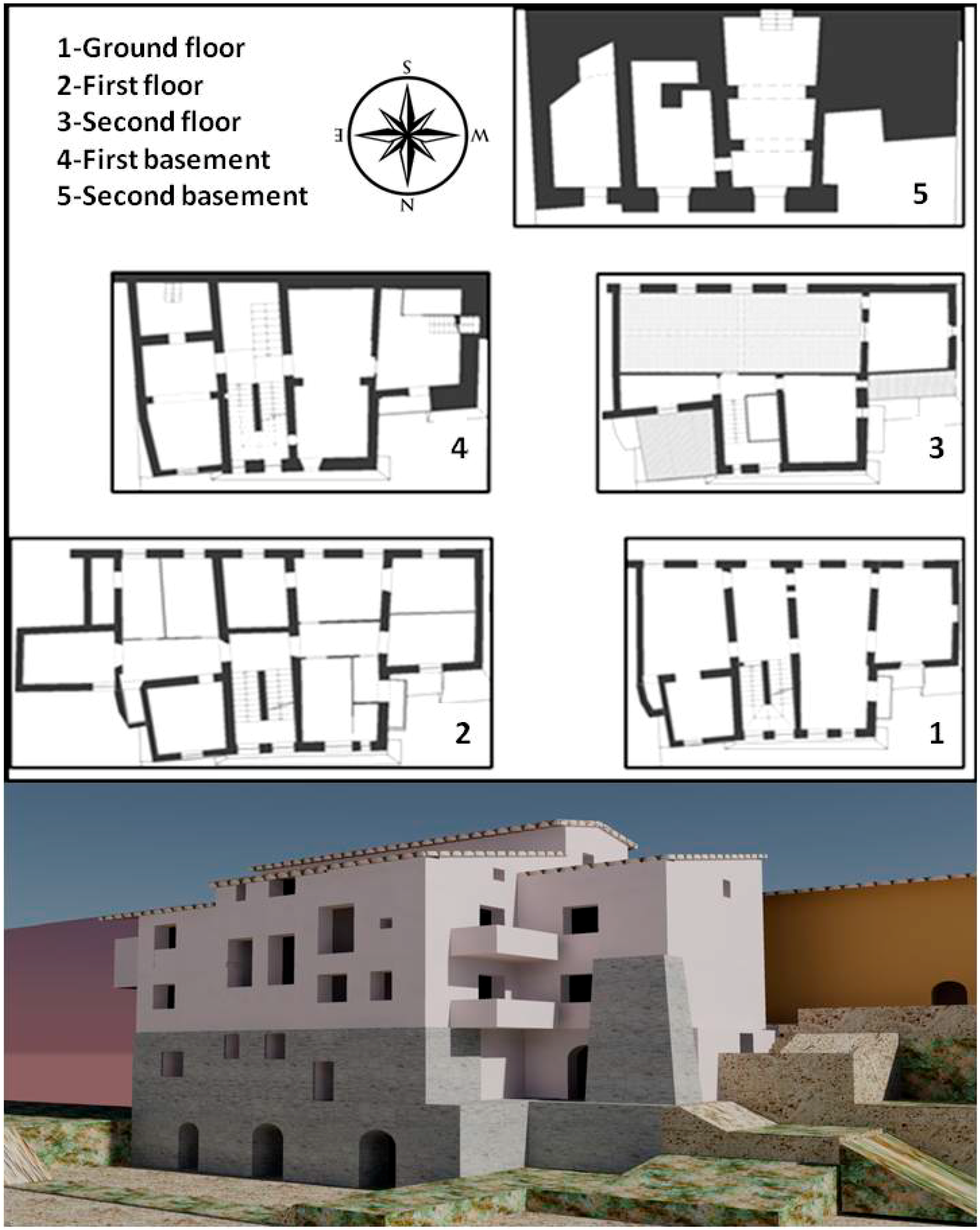
  • The old building (Figure 1) is composed of five floors (three over ground and two in the basement), presenting a complex geometry. The structure is completely made of tuff, with large walls characterized by a thickness ranging from 10 cm to 170 cm. The west side is connected to the ground for a small part. The east side of the structure is close to another building. The construction dates back to 800;
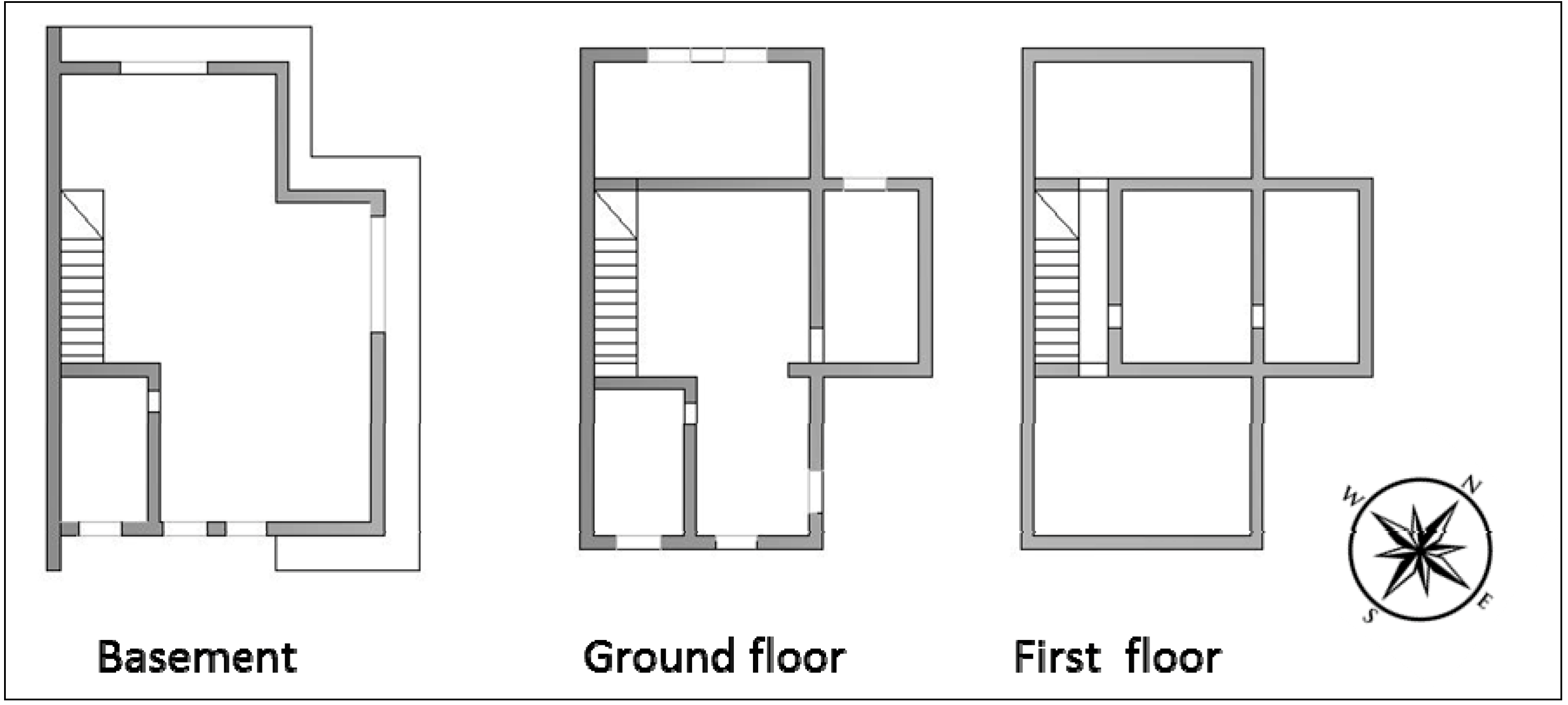
  • The house (Figure 2) is composed by three floors (two over ground and one in the basement). External wall thickness is equal to 30 cm. At the first floor there are no windows on the vertical surfaces (there are only three windows on the roof). The basement is characterized by a gap all around the building able to guarantee a thermal insulation from the ground. The construction year is 2005;
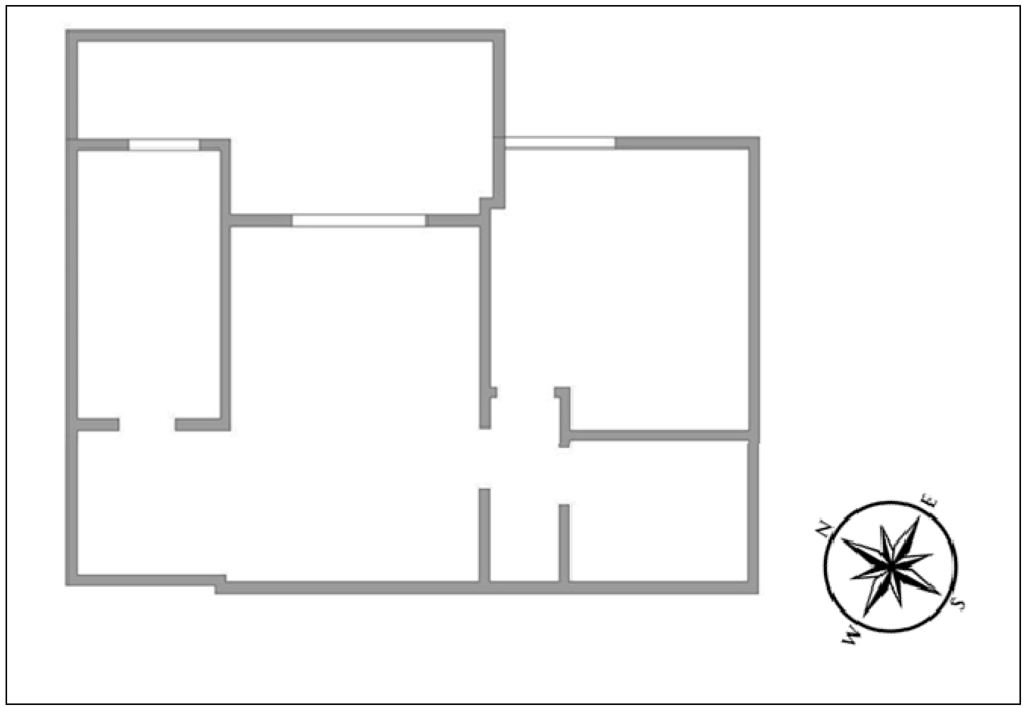
  • The flat (Figure 3) is developed on a single floor, specifically it is the top floor of a building. For this reason the heat dispersion concerns only the roof, the west side and the south side. The construction year is 1988.
Figure 1 shows the historical building. Figure 2 and Figure 3 show the house and flat layouts, respectively. Table 1, Table 2 and Table 3 list the materials employed to build the structures and their thermophysical properties.
Figure 1. Planimetric and 3D representation of Historical building.
Sustainability 06 05311 g001
Figure 2. Planimetric representation of House.
Sustainability 06 05311 g002
Figure 3. Planimetric representation of Flat.
Sustainability 06 05311 g003
Table 1. Historical building’s material characteristics.
MaterialsThermal Conductivity (W/m K)Specific Heat Capacity (kJ/kg K)Mass Density (kg/m3)
Tuff0.6301.3001500
Concrete1.2631.0002000
Brick0.5000.840840
Roof’s spruce beam0.1201.600450
Plaster0.9000.9101800
Brick0.3250.8401070
Roof’s spruce beam0.1700.9201200
Perforated brick1.0000.8402000
Insulating material0.5000.840840
Shingle0.1201.600450
Perforated brick0.9000.9101800
Insulating material0.3250.8401070
Tile0.8400.8401700
WindowsCharacteristicsThermal Transmittance (W/m2K) G-value
FrameAluminium2.27-
Double insulated glassDouble glazing 4/16/4 with air2.830.755
Table 2. House’s material characteristics.
MaterialsThermal Conductivity (W/m K)Specific Heat Capacity (kJ/kg K)Mass Density (kg/m3)
Plasterboard0.1600.840950
Light concrete0.1700.840500
Wood0.1201.600450
Tile10.8402000
Light concrete basement21.0002400
WindowsCharacteristicsThermal Transmittance (W/m2K)G-value
FrameAluminium2.27-
Double insulated glassDouble glazing 4/16/4 with air2.830.755
Table 3. Flat’s material characteristics.
MaterialsThermal Conductivity (W/m K)Specific Heat Capacity (kJ/kg K)Mass Density (kg/m3)
Plasterboard0.1600.840950
Light concrete0.3200.8401000
Insulating material0.1700.9201200
WindowsCharacteristicsThermal Transmittance (W/m2K)G-value
FrameAluminium2.27-
Double insulated glassDouble glazing 4/16/4 with air2.830.755
The three building types considered in this study are characterized by different constructive schemes. The tuff’s walls, that characterize the old building, are thick and massive; consequently, the structure has a significant thermal inertia. On the other hand, house and flat are more recent and, for this reason, their walls are characterized by lower transmittance values in spite of small thickness.

2.2. Modeling

Employing a simulation software able to evaluate the annual energy demand of a building can be a reliable and effective method if the obtained results are sufficiently representative of the actual structure behavior. In this work two different approaches have been tested: steady-state and dynamic conditions. The first one has been studied by means of Aermec MC11300 [18] code: this is a semi-stationary software, based on the simplified procedure shown in the UNI EN ISO 13790. The second one has been performed by using TRNSYS [19], that is a well-known dynamic software, based on the transfer function method developed by Mitalas [14].
Using MC11300 the generated models are characterized by a lack of details; it is hard to design a roof with a particular geometrical characteristics and it is also hard to define all the details of the ground on which the structure is built.
TRNSYS applies the transfer functions relationships and it is able to provide the energy demands for each hour during the day. Using this software it is possible to overcome the limitations previously mentioned, exploiting different characteristic. First of all, TRNSYS is based on complete weather-data containing hourly variation of temperature, solar radiation, wind velocity and relative humidity. Consequently, the annual energy demand will be calculated as a sum of hourly load values. Moreover, materials mass density and specific heat capacity are employed to appreciate the building thermal inertia. Finally, more detailed building structural models can be used as input, which can provide more insightful information. This more accurate modeling is made by the two different parts of the software: TRNSYS Build, which allows us to reproduce the building model and TRNSYS Studio which is employed to simulate the energy demand using as input the external environmental conditions.
The thermal properties of the building materials (Table 1, Table 2 and Table 3) were used in Aermec MC11300 and TRNSYS as input and the structures geometry were reproduced. The models generated through MC11300 and TRNSYS are comparable in terms of opaque walls thermal transmittance, transparent surfaces thermal transmittance, windows solar gain factor and geometrical features. Aermec MC11300 is characterized by a compiling interface with a rigid structure: users can fill in the required fields. TRNSYS is divided in two different parts: an interface, which is represented by TRANSYS Build and, as previously mentioned, TRNSYS Studio that is made up by several “Types” (small objects written in Fortran or C++), able to achieve specified tasks and connected together.
It is evident that to carry out a comparison between the different calculation codes, the simulations have to be performed considering the same geographical position (Rome, in our study). Moreover, aiming to make the two models comparable, internal gains and ventilation systems were not taken into account.

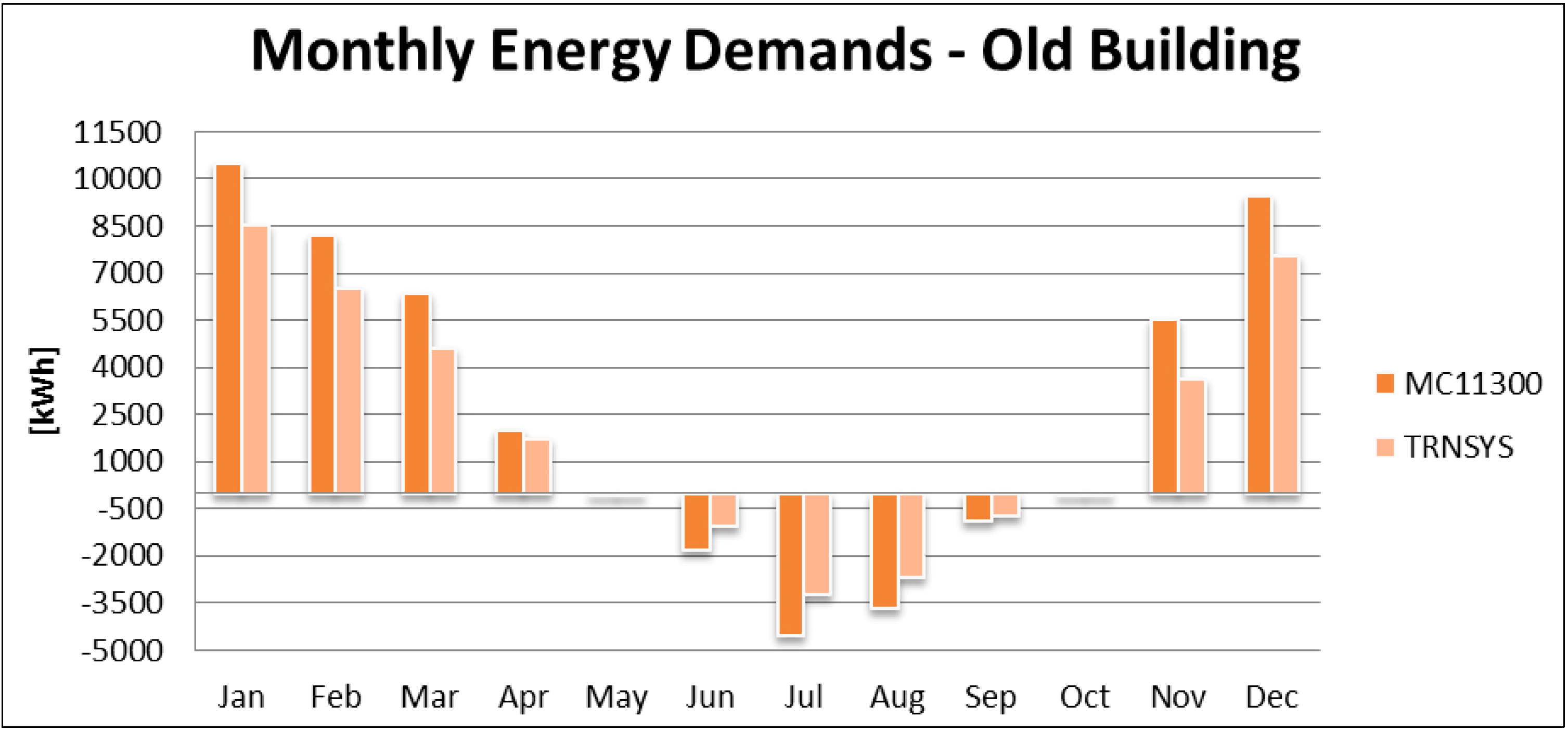
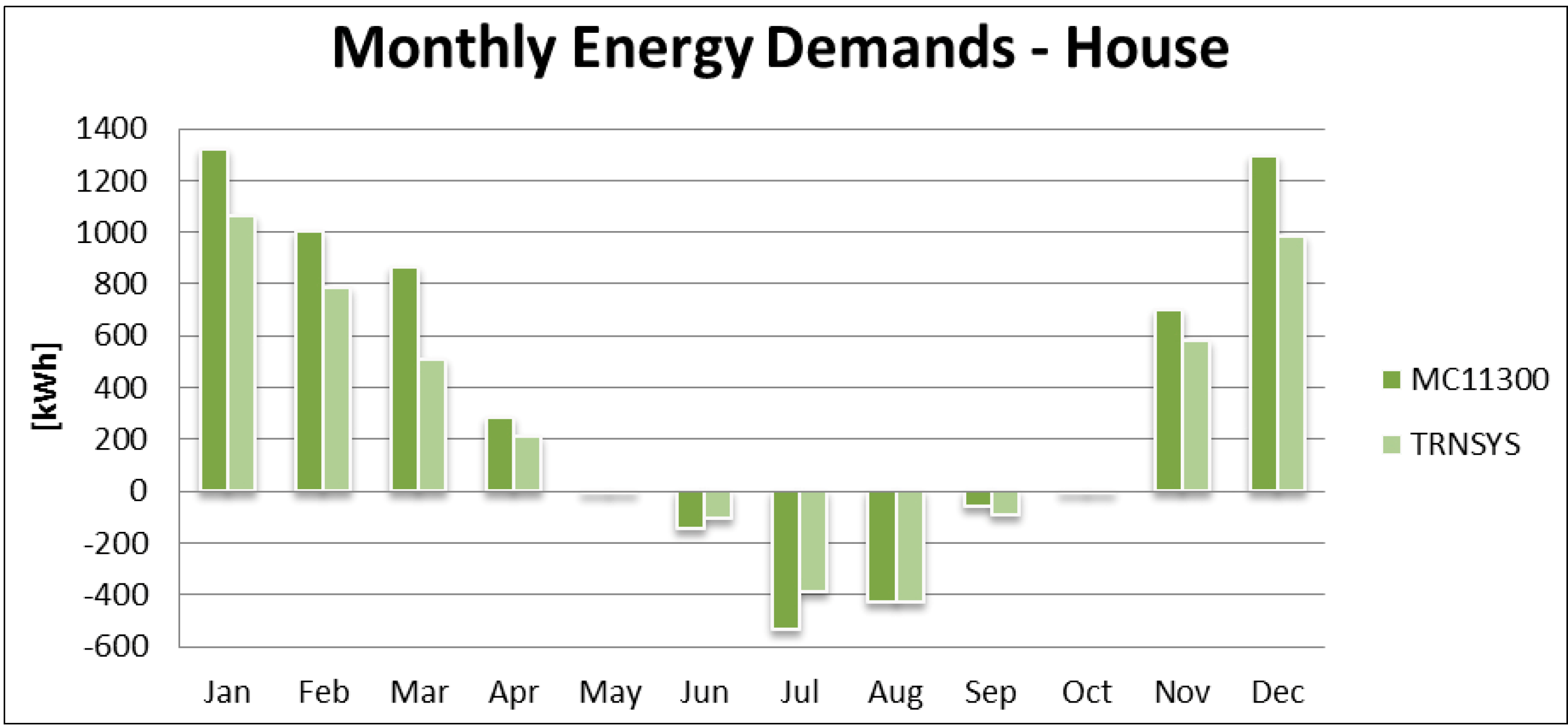
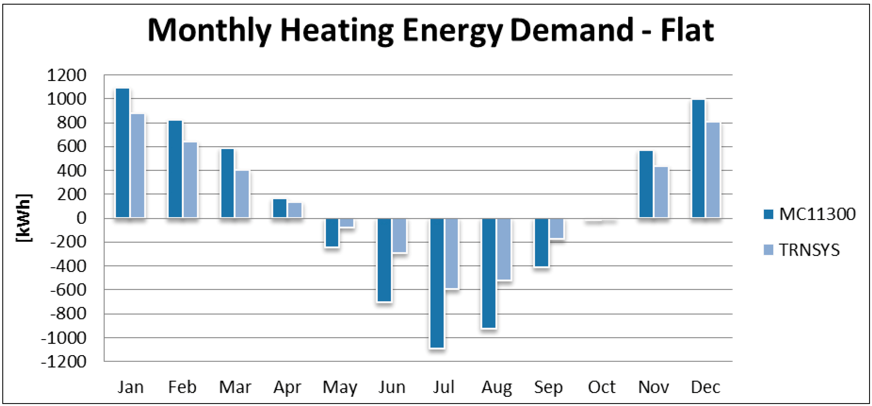
3. Results and Discussion

Starting from these data, simulations under steady-state and dynamic conditions were performed with the MC11300 software and with TRNSYS, respectively. It is possible to distinguish between the heating demand QH ,nd, which is referred to the winter, and the cooling demand QC ,nd, which is related to the summer. This allowed us to highlight the differences between the energy demand values, that were calculated both through the stationary software and the dynamic one (Table 4 and Table 5).
Table 4. Energy demands using different calculation codes.
MC11300TRNSYS
QH, nd (kWh)QC, nd (kWh)QH, nd (kWh)QC, nd (kWh)
Old Building4195710697328607764
House5425 112841831014
Flat4237337833451582
Table 5. Differences between energy demands.
kWh Difference (MC11300-TRNSYS)Percentage Difference compared to TRNSYS (%)
Old BuildingQH, nd909727.7
QC, nd293337.8
HouseQH, nd124229.7
QC, nd11411.2
FlatQH, nd89226.6
QC, nd1796113.5
As it is shown in Table 5, considering the data referred to the old building, the heating demand calculated through MC11300 is higher than the same demand obtained through TRNSYS. This difference, equal to 27.7%, is related to a different way to take into account the inertial behavior of the structure. MC11300 overestimates the heating energy demand, not considering the walls heat storage. Moreover, the structure basement and other walls are in contact with the ground and TRNSYS uses a specific “Type” to simulate this condition. Cooling demand values obtained with TRNSYS are lower compared with the values calculated under semi-stationary conditions: the dynamic software takes into account the structure’s thermal inertia and in particular the fact that during the night, the building releases the heat stored during the day. During the cooling time, the percentage difference grows up to about 38%.
Regarding the house and flat (Table 5), MC11300 overestimates the heating energy demand, with a percentage difference of about 30%. On the other hand, house’s cooling values are similar but, analyzing the data regarding the flat, it is possible to observe a very large percentage difference equal to 113.5%.
The energy demand was further analyzed by calculating its monthly instead of yearly distribution, in order to obtain more specific information about the calculation code differences. Figure 4, Figure 5 and Figure 6 show the monthly energy demands of the old building, house and flat, respectively. It is possible to observe that TRNSYS values are essentially always lower than MC11300 values and this is due to the software capability to take into account the dynamic thermal storage during plant operation.
Figure 4. Old Building monthly energy demands.
Sustainability 06 05311 g004
Figure 5. House monthly energy demands.
Sustainability 06 05311 g005
Figure 6. Flat monthly energy demands.
Sustainability 06 05311 g006
Finally, the monthly percentage differences between energy demands were calculated and analyzing the Figure 5 and Figure 6 it shows that the values (percentage differences comparing TRNSYS results to MC11300 results). During the winter, the percentage differences range between 13.5% (old building–April) and 68.6% (house–March). On the other hand, during the summer, they range from 0.2% (house–August) to 330% (old building–May).
As it is important note that the largest percentage differences are shown in May and October, but, it is worth- to notice that the energy demand values–in these months–are negligible compared to the other summer months. Thus, such high percentage differences do not have to be considered very significant. All the reported results highlight the need to employ more effective simulation tools for both winter and summer energy demands.
It is therefore possible to affirm that different calculation codes can lead to different results in terms of building energy performance. Simplified approaches are poorly representative of a real building performance (especially during the summer); thus, stationary software could lead to inaccurate building energy performance estimation and a consequent rough evaluation of the coupling between building and plant.

4. Conclusions

The proposed study wants to point out numerical differences arising from the use of a semi-stationary and a dynamic calculation code applied to different building types. The differences of these three kinds of architectures are related not only to structural characteristics (possible contacts with the ground or gaps around the building) but also take into account the inertial structure properties on annual energy demand variations.
This study is important to better understand the necessity of using more complex tools to evaluate and to assess the buildings energy efficiency and, consequently, a step towards a method of investigation which allows a better building-plant coupling.
Taking into account a detailed calculation of heat flows–hour by hour–and building’s inertial capacity, it is possible to assess significant variations of seasonal energy demands. In order to highlight the limitations of a simplified procedure to define buildings energy behavior, an old building, a house and a flat (all placed in the same climatic area and geographical position–Rome) were modeled and their behaviors were analyzed both under steady-state and dynamic conditions. At the beginning of the study, in order to consider the steady-state part of climatic phenomena, the software MC11300 has been used; then, the program TRNSYS, able to appreciate the climate changes over time, has been employed. Through these software applications the building's geometries and materials thermal properties have been reproduced. Finally, the obtained numerical results have been compared. Through the simulation of the buildings energy performance, some differences were found between energy demand values calculated through the stationary software and the dynamic one. These differences, for some months of the year, can be very large and they occur regardless of the building type and the inertial properties. For this reason, it is possible to assess that simplified approaches—simplified European Standard—are poorly representative of a real building performance, especially during the summer. Stationary codes are not able to reproduce faithfully the energy behavior of the building, with a possible imprecise building energy certification. According to the results, a semi-stationary energy analysis should be placed side by side with a dynamic one because average differences of about 30% are definitely not negligible when we want to study the energy behavior of a building.
Finally, in this study we tried to get a general confirmation of the results derived from other studies, which developed a comparison between stationary and dynamic models in a specific case study [15,16] by comparing them with experimental data. We have analyzed several buildings totally different and we tried to get the overall results comparing the results obtained from stationary and dynamic models for each of them. In particular, we can generally say that regardless of the type, the use and the year of construction, stationary software that refer to the UNI TS 11300, about a 25%–30% overestimate of the energy demand for heating, and still give results completely unreliable to predict the energy demand for cooling.

Author Contributions

Roberto de Lieto Vollaro and Luca Evangelisti designed this research; Gabriele Battista, Caludia Guattari and Carmine Basilicata performed the calculations and analyzed the data. Luca Evangelisti wrote the paper.

Conflicts of Interest

The authors declare no conflict of interest.

References

  1. Casals, X.G. Analysis of building energy regulation and certification in Europe: Their role, limitation and differences. Energ. Buildings 2006, 38, 381–392. [Google Scholar] [CrossRef]
  2. De Lieto, V.R.; Calvesi, M.; Battista, G.; Evangelisti, L.; Botta, F. Calculation model for optimization design of the low impact energy systems for the buildings. Energ. Procedia 2014, 48, 1459–1467. [Google Scholar] [CrossRef]
  3. Crawley, D.B.; Hand, J.W.; Kummert, M.; Griffith, B.T. Contrasting the capabilities of building energy performance simulation programs. Buildings Environ. 2008, 43, 661–673. [Google Scholar] [CrossRef] [Green Version]
  4. Dounis, A.I.; Caraiscos, C. Advanced control systems engineering for energy and comfort management in a building environment—A review. Renew. Sust. Energ. Rev. 2009, 13, 1246–1261. [Google Scholar] [CrossRef]
  5. Zhu, N.; Zhenjun, M.; Shengwei, W. Dynamic characteristics and energy performance of buildings using phase change materials: A review. Energ. Convers. Manage. 2009, 50, 3169–3181. [Google Scholar] [CrossRef]
  6. Perez-Lombard, L.; Ortiz, J.; Gonzalez, R.; Maestre, I.R. A review of benchmarking, rating and labeling concepts within the framework of building energy certification schemes. Energ. Buildings 2009, 41, 272–278. [Google Scholar] [CrossRef]
  7. Asdrubali, F.; Bonaut, M.; Battisti, M.; Venegas, M. Comparative study of energy regulations for buildings in Italy and Spain. Energ. Buildings 2008, 40, 1805–1815. [Google Scholar] [CrossRef]
  8. Henninger, R.H.; Witte, M.J. Energy Plus Testing with Building Thermal Envelope and Fabric Load Tests from ANSI/ASHRAE Standard 140-2004; U.S. Department of Energy Efficiency and Renewable Energy Office of Building Technologies: Washington, DC, USA, 2004.
  9. Ferrari, S. Building envelope and heat capacity: Re-discovering the thermal mass for winter energy saving. In Proceedings of the 2nd PALENC & 28th AIVC Conferences, Crete Island, Greece, 27–29 September 2007.
  10. Ferrari, S.; Baldinazzo, M. Assessment of the energy performance of buildings: From simplified procedures to dynamic analysis. In Proceedings of AICARR, Padova, Italy, 18 June 2009.
  11. De Lieto, V.R.; Evangelisti, L.; Carnielo, E.; Battista, G.; Gori, P.; Guattari, C.; Fanchiotti, A. An Integrated Approach for an Historical Buildings Energy Analysis in a Smart Cities Perspective. Energ. Procedia 2014, 45, 372–378. [Google Scholar] [CrossRef]
  12. Balocco, C.; Gori, V.; Marmonti, E.; Citi, L. Building-plant system energy sustainability. An approach for transient thermal performance analysis. Energ. Buildings 2012, 49, 443–453. [Google Scholar] [CrossRef]
  13. Aste, N.; Angelotti, A.; Buzzetti, M. The influence of the external walls thermal inertia on the energy performance of well insulated buildings. Energ. Buildings 2009, 41, 1181–1187. [Google Scholar] [CrossRef]
  14. Mitalas, G.P. Transfer function method of calculating cooling loads, heat extraction and space temperature. Ashrae J. 1973, 14, 54–56. [Google Scholar]
  15. Asdrubali, F.; Cotana, F.; Messineo, A. On the evaluation of solar greenhouse efficiency in building simulation during the heating period. Energies 2012, 5, 1864–1880. [Google Scholar] [CrossRef]
  16. Milone, A.; Milone, D.; Pitruzzella, S. Asset rating: Disagreement between the results obtained from software for energy certification. In Proceedings of the Eleventh International IBPSA Conference, Glasgow, UK, 27–30 July 2009.
  17. Energy performance of buildings. Directive 2002/91/EC, 2002.
  18. Comitato Termotecnico Italiano (CTI). Energy Performance of Buildings–Part 1: Determination of Thermal Energy Demand for Air Conditioning in Winter and Summer; UNI TS 11300-1:2008; CTI: Milan, Italy, 2008. [Google Scholar]
  19. Comitato Termotecnico Italiano (CTI). Energy Performance of Buildings–Calculation of Energy Use for Heating and Cooling; EN ISO 13790; CTI: Milan, Italy, 2008. [Google Scholar]

