Article

Dynamics of Multi-Scale Intra-Provincial Regional Inequality in Zhejiang, China

1
Department of Land Management, Zhejiang University, Hangzhou 310029, China
2
Key Laboratory of Carrying Capacity Assessment for Resource and Environment, Ministry of Land and Resources, Beijing 101149, China
3
Center for Yellow River Civilization and Sustainable Development, Henan University, Kaifeng 475001, China
4
Department of Geography, Kent State University, Kent, OH 44242, USA
5
College of Geography and Tourism, Hainan Normal University, Haikou 571158, China
6
Department of Geography & Geology, Sam Houston State University, Huntsville, TX 77340, USA
*
Author to whom correspondence should be addressed.
Sustainability 2014, 6(9), 5763-5784; https://doi.org/10.3390/su6095763
Submission received: 29 April 2014 / Revised: 28 July 2014 / Accepted: 1 August 2014 / Published: 29 August 2014
(This article belongs to the Section Economic and Business Aspects of Sustainability)

Abstract

:
This paper investigates regional inequality in a multi-scale framework, using Exploratory Spatial Data Analysis, based on the per capita Gross Domestic Product (GDP) of counties and municipalities within the Zhejiang province in China between the years of 1990 and 2010. A Spatial Markov Chain is used to identify the dynamics of regional wealth disparity in Zhejiang. The results show that the regional inequality of Zhejiang is sensitive to the geographic scale of the analysis. In addition, the inter-county inequality shows an inverted-U shape pattern. At the same time, the inter-municipality inequality displays a more consistently upward trend, and the evolution of the interregional inequality is relatively stable over time. The regional inequality is more significant at finer (larger) spatial scales. The decomposition of the Theil Index shows that the contribution of the inequalities between Northeast Zhejiang and Southwest Zhejiang increased. The increasingly larger values of the Global Moran’s I show that there is an intensifying spatial aggregation of economic development. The comparison of the traditional Markov transition matrix and the Spatial Markov transition matrix illustrates how the relative wealth or poverty of neighboring counties make a significance difference in wealth in a given county as measured using domestic GDP per capita in Zhejiang province. This space-time analysis is valuable for policy making towards sustainable economic development in China given the soaring spatial inequality.

Graphical Abstract

1. Introduction

Problems with state socialism in China during Mao’s era prompted the launch of economic reforms in 1978, and since then, China has been undergoing a profound process of triple transition (decentralization, globalization, and market reforms) [1,2,3,4]. Over the past three decades, China’s transition towards a market-oriented globalized economy has been unrelenting and spectacular with an annual growth rate of 9.9%. China’s total GDP has increased from 364.52 billion yuan in 1990 to 40.12 trillion yuan in 2010, its GDP per capita also increased from 381 yuan in 1990 to 29,992 yuan in 2010 [5]. Even adjusted for inflation the growth in wealth has been impressive. However, behind the economic success in China, the country also faces serious challenges from imbalanced growth and the potential for intensifying social injustice because of the differences in the level of infrastructure development, proximity to markets and coastal areas, natural resource endowments, demographic factors and regional policy [1]. Spatially evident inequalities and instability in the regional wealth distribution has been one of the most salient features of regional development in China. In 2010, Shanghai’s GDP per capita (76,074 yuan) was the highest in the country, while the lowest was in Guizhou (a small mountainous inland province near Vietnam), where it was only 13,119 yuan [5].
To put this inequality in a global perspective, the disparity in per capita income in 2011 between and the perennially poorest U.S. State of Mississippi (at $20,670) and the richest state of Connecticut (at $37,807) was far less stark. Disparities in most other developed countries are less pronounced than in the U.S. The richest Australian state (Western Australia) had a per capita GDP of 26,962 (in Australian Dollars) while the poorest state (Tasmania) had a per capita GDP of 18,779 (in Australian Dollars) in 2012. Even smaller disparities are found in Europe’s most developed countries. In Holland, the richest region (Hovedstaden) had a per capita GDP of $55,616 while the poorest region (Nordjylland) had a per capita GDP of $48,268 in 2010. In 2013 in Norway, the world’s wealthiest country, the richest region (Oslo) had a per capita GDP of approximately 254,000 (Norwegian Kroner), while the poorest region (Ostmark) had a per capita GDP of 211,000 (Norwegian Kroner). Thus, the wealthiest region (province) in China on a per capita basis was 5.8 times richer than the poorest, this compared to 1.8 times in the U.S., 1.4 times in Australia and 1.2 times in Holland and also in Norway. Of course, GDP per capita is not the only, or even the best possible measurement of wealth, especially personal wealth. In developed countries there are several other measures available in particular household income and personal income these can be adjusted for income before or after taxes. However, whatever index of wealth is chosen, wealth disparities in the most developed nations between rich and poor regions are relatively small. Possessing such small income disparities are an index of national and regional development and are used for example as one of many factors in determining ranking in the United Nation’s human development index where in 2013 Norway was ranked first, Australia second, the U.S. third, Holland fourth and China was ranked 101st out of 187 nations [6].
Achieving a more balanced territorial distribution of wealth is among the challenges for regional policy design in China. Issues of regional inequality have been particularly important in China, which inherited an unbalanced economy from its imperial history and as a vestige of a past troubled by colonialism, civil war and pestilence. Since regional inequality may threaten national unity and social stability, it has become a burning issue in China, attracting considerable attention from policy makers and scholars [3]. Geographers are involved in these discussions and are intrigued by questions, such as identifying regions or places that are rich and others that are poor and determining causal factors. Questions such as: Is geographic inequality widening and why? What can be done to reduce poverty and spatial inequality? Will wealth be shared by people in all regions and places?
In contrast to Holland and to a lesser extent Norway, China is characterized by vastness in size. In contrast to Australia and even the U.S., it has a huge and ethnically and linguistically diverse population. Thus regional inequalities exist among provinces and groups of provinces but also within provinces. This means that research on inequality in China should also be conducted within a province. In order to understand inequality, research must be conducted at finer-scales than nationally. Useful analysis can therefore be conducted at the intra-provincial level [2,7]. This paper selects three geographical scales (county, municipality and region) to measure wealth inequality in Zhejiang province during the period from 1990 to 2010. In addition, it also analyzes the spatial aggregation and dynamics of wealth inequality using spatial autocorrelation and spatial Markov chain.

2. Literature Review, Research Areas and Methods

2.1. Literature Review

Regional inequality has been the subject of intense debates among the proponents of the convergence, divergence, inverted-U, and endogenous growth theories. A great deal of empirical work has been conducted in the late 1960s and the 1970s to test the neoclassical convergence theories [1,2]. While some supported the convergence and inverted-U theories, others found there was a lack of convergence and that regional inequality even increased in some countries [4]. The findings of persistent poverty and inequality prompted new thinking on development and inequality, and the promise of neoclassical convergence received severe critiques from many scholars [7]. Theories based on cumulative causation, dependency, and neo-Marxism became poplar alternatives at this time. A renewed interest in regional inequality has occurred since the early 1990s. The new convergence theory developed by [8,9] has become a mainstream theory for analysis of economic growth and regional inequality.
China’s mounting importance in the world economic system since the launch of reforms in the late 1970s has long been the subject of intense academic debates, in terms of its remarkable growth and poverty reduction. Such phenomenal development has been a hallmark of China’s growth, and has been gaining attentions and recognition [3]. The speed and unevenness of economic restructuring and development in favor of specific regions, is truly unprecedented and merits a careful examination and assessment both theoretically and methodologically. Scholars have been intensely debating the impacts of the reform on regional convergence and inequality [1,3]. Research has revealed that patterns of regional inequality differ with geographical scales, thus creating a multi-scalar typology of regional inequality in China. Multi-scale and multi-mechanism approach has been adopted, with a synthesis of global, state and local forces in understanding the process of regional development [1,10].
China has been the fastest-growing major economy in the world for the past three decades with an average annual GDP growth rate about 10%. However, there are various layers and dimensions to the transition, and scholars have been very concerned with the social and spatial ramifications of reforms. Research on China has unfolded a complex landscape of regional inequality, and the significance of globalization, institutions, and local agents in regional development [11,12].
The investigation of regional inequality is sensitive to geographical scales [1]. For example, in the study of regional inequality in Zhejiang, due to the difference in selecting research scales, the results are different (Table 1). Investigating the characteristics and evolution of the regional inequality within a wealthy province like Zhejiang yields insights valuable for revealing the internal mechanism of regional disparities within this and other Chinese provinces. Gaining these insights in turn fosters the development of policy solutions directed at reducing wealth inequality.
Table 1. Some previous studies on Zhejiang.
AuthorsSpatial Scales
Ye and Chen[13]District
Luo[14]Municipality
Wei and Ye[1]County and Municipality
However, one must exercise care in the study of regional inequality in Zhejiang, because the apparent results are quite sensitive to scale dependent factors. Ye and Chen use the District as the research scale in a study of regional inequality in Zhejiang between 1990 and 2004, and Zhejiang is divided into three regions—the Northeast Zhejiang region, the Wentai (Wenzhou and Taizhou) region, and the Jinquli (Jinhua, Quzhou, and Lishui) region [13]. They find that the regional inequality shows a U-shape pattern, it declines from 1990 to 1996 and then rises from 1997 to 2004. Luo adopts 11 municipalities as the research scale, and claims that the regional inequality in Zhejiang has been constantly increasing, and especially worsened since 2000. Luo argues that inequality has been very high and a widening gap between rich and poor cities has been further intensified [14]. However, Wei and Ye utilize two research scales (county and municipality) to measure the regional inequality in Zhejiang, and find that the inter-county inequality in Zhejiang rises constantly and the inter-municipality inequality demonstrates an inverted-U shape pattern: it grows constantly before 1990 and drops after 1990 [1]. These would appear to be contradictory results. But they in fact depend on the exact years, cities and counties chosen as well as scale dependent factors.
The spatial econometric and spatial statistics literatures offer many powerful tools for analyzing spatial dependence and heterogeneity in spatial patterns of economic and other phenomena [15,16,17]. Exploratory spatial data analysis (ESDA) is a set of techniques aimed at describing and visualizing spatial distributions, at identifying atypical localizations or spatial outliers, at detecting patterns of spatial association, clusters or hot spots, and at suggesting spatial regimes or other forms of spatial heterogeneity [18,19,20]. These methods provide measures of global and local spatial autocorrelation. A positive value indicates that the attribute value change of the cell has the same trend with that of its adjacent cells and vice versa. The traditional Markov chain approach can be further used for the analysis of the evolution over time of regional convergence (or divergence). However, as this method distinguishes the different regions as “islands” ignoring the spatial interaction between regions, it can’t reveal the spatial characteristics of regional convergence. The Spatial Markov chain is the combination of the traditional Markov chain and the concept of a “spatial lag” [21,22]. Application of these methods to questions of regional inequality has yielded a number of new insights as to the role of space and regional context in economic outcomes [17,18,19,20,21,22,23,24,25].

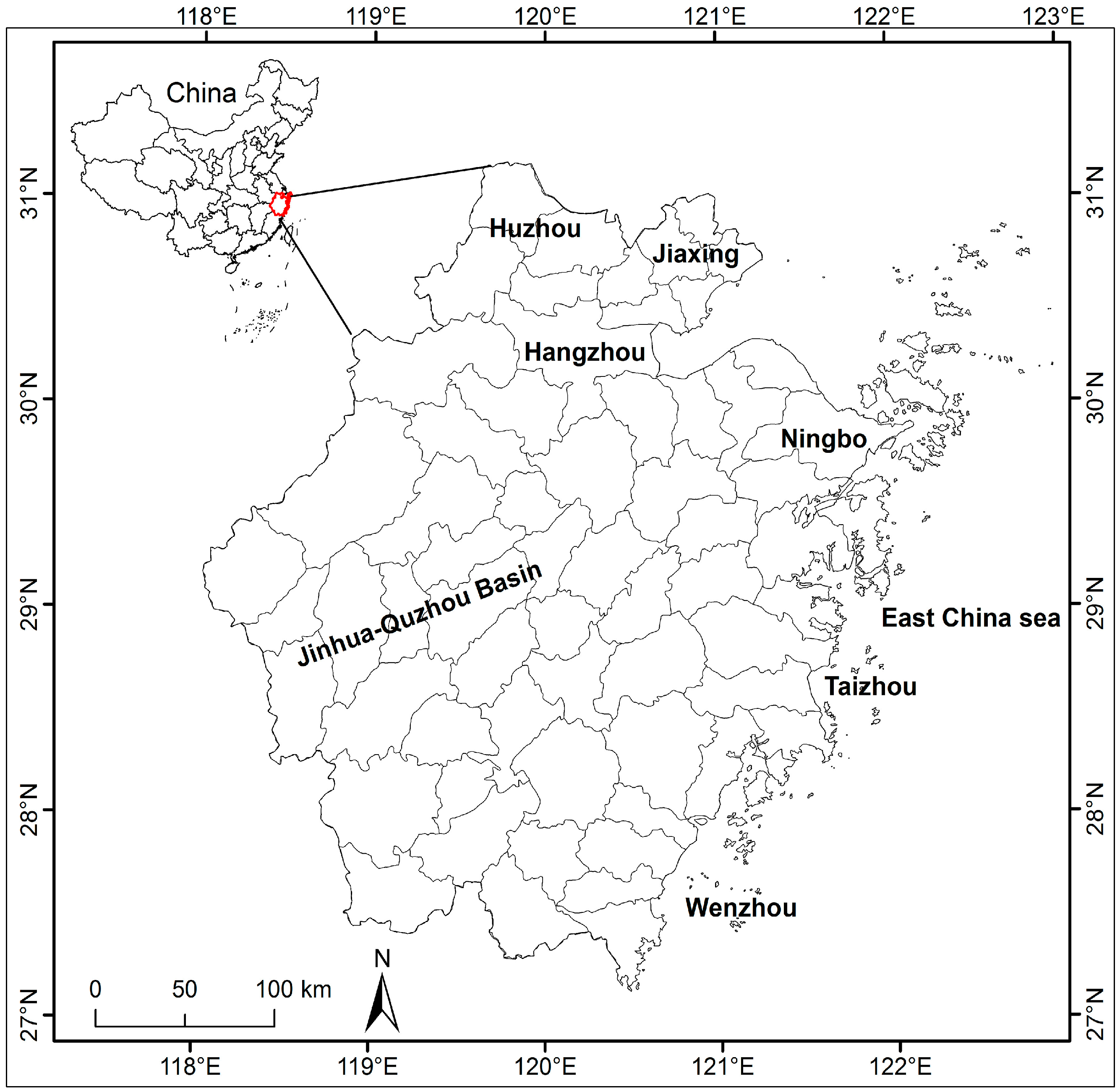
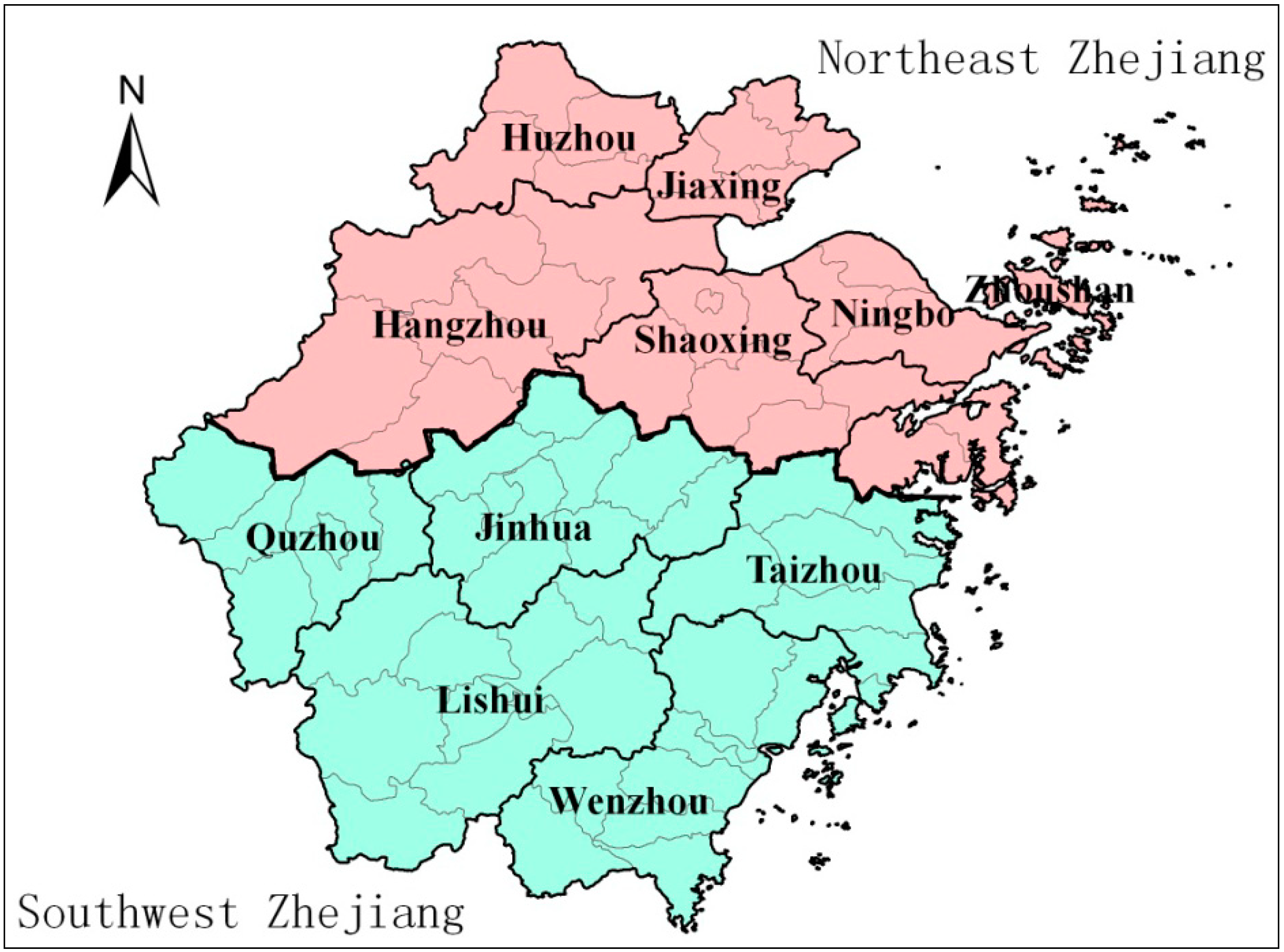
2.2. Research Areas and Research Unit Division

Zhejiang province is an important eastern Chinese province. It has long been noted for production of green tea, silk and aquaculture. As shown in Figure 1, Zhejiang province is located in the Yangtze River Delta region, in Eastern China and neighbors Shanghai (Figure 1). With a population of 47.4795 million (3.54% of China’s total population) in 2010, the province covers 104,141 square kilometers, 1.08% of China’s territory (Table 2). Zhejiang is one of the most developed provinces in China, generating 2772.231 billion yuan of GDP in 2010, ranking fourth among China’s 31 provinces (NBSC, 2011). Its GDP per capita also increased from 331 yuan in 1978 to 51,711 yuan in 2010 with an annual growth rate of 11.2% [26]. Since 1979 it has followed an entrepreneurial economic development model that has made it a prosperous center of small industries geared to export of consumer goods, in particular toys and textiles. Some commentators have lauded its economic model.
Figure 1. Location of Zhejiang province.
Sustainability 06 05763 g001
Within Zhejiang province, the imbalance of economic development is very obvious. For example, in 2010, for the 11 municipalities of Zhejiang province, Ningbo’s GDP per capita is 3.52 times of Lishui’s; while for the 58 counties (including rural counties and county-level cities) of Zhejiang province, Shaoxing County’s GDP per capita is 6.90 times of Jingning She Autonomous County’s [26]. The economic development of Zhejiang mainly concentrates in the Northeast and coastal areas, while the inland areas of Southwest Zhejiang lag far behind other regions. Investigating the characteristics and evolution of the regional inequality within Zhejiang has important significance for revealing the internal mechanism of regional disparities within Zhejiang and putting forward the policy proposal of inequality-reducing.
As shown in Figure 1, Zhejiang province is located in the Yangtze River Delta region, East China and neighbors Shanghai. With a population of 47.4795 million (3.54% of China’s total population) in 2010, the province covers 104,141 square kilometers, 1.08% of China’s territory (Table 2). Zhejiang is one of the most developed provinces in China, generating 2772.231 billion yuan of GDP in 2010, ranking fourth among China’s 31 provinces [5]. Its GDP per capita also increased from 331 yuan in 1978 to 51,711 yuan in 2010 with an annual growth rate of 11.2% [26].
Table 2. Development indicators of Zhejiang province, 2010.
ZJ% of ChinaNortheast% of ZJSoutheast% of ZJ
Population (million)47.47953.5424.004650.5623.474849.44
Land area (km2)104,1411.0845,86444.0458,27755.96
GDP (billion yuan)2772.2316.911815.36267.97888.0332.03
Investment in fixed assets (billion yuan)1237.6044.45881.40671.22345.12128.78
Exports (U.S. $billion)180.46511.44137.23376.0443.24723.96
FDI (U.S. $billion)11.0017510.4110.2290892.980.760317.02
Local fiscal expenditure (billion yuan)2857.833.871870.4965.45987.3434.55
Local fiscal revenue (billion yuan)2371.855.841730.6372.97641.2227.03
Source: Zhejiang Province Statistics Bureau [26]; ZJ = Zhejiang.
Within Zhejiang province, the imbalance in economic development is very obvious. For example, in 2010, for the 11 municipalities of Zhejiang province, Ningbo’s GDP per capita was 3.52 times of that of Lishui’s; while for the 58 counties (including rural counties and county-level cities) of Zhejiang province, Shaoxing County’s GDP per capita was 6.9 times that of Jingning She Autonomous County’s [1]. The economic development of Zhejiang is mainly concentrated in the Northeast and coastal areas, while the inland areas of Southwest Zhejiang lagging far behind other regions [7,27].
In Zhejiang in 2010, there were 11 municipalities and 90 county level administrative units including 32 municipal districts and 58 counties (including 35 rural counties, 22 county-level cities and one Autonomous County). Zhejiang was traditionally divided into Southwest Zhejiang (Wenzhou, Jinhua, Quzhou, Taizhou, Lishui municipalities) and Northeast Zhejiang (Hangzhou, Ningbo, Jiaxing, Huzhou, Shaoxing, Zhoushan municipalities) as portrayed in Figure 2. As shown in Table 2, the economic development of Zhejiang province mainly is concentrated in the six municipalities in the Northeastern portion of Zhejiang. There is a significant North-South divide in development. In 2010, the ratio of GDP per capita in Northeast Zhejiang compared to that in Southwest Zhejiang was 2:1 [1]. With a population of 24.0046 million (50.56% of the province), the Northeastern portion of Zhejiang produced 67.97% of the total GDP in Zhejiang. In terms of investment in fixed assets, exports, local fiscal revenue, local fiscal expenditure and so on, Northeast Zhejiang was far ahead of Southwest Zhejiang, and it also took a massively disproportionate share of the foreign direct investment (FDI) made in the province, in fact 92.98% of it.
Figure 2. Regional divisions
Sustainability 06 05763 g002
This paper selects three types of spatial scales as the spatial units of analysis: (1) Counties: the existing 69 county level spatial units, including rural counties, county-level cities and municipal districts (where different districts are unified as a urban district); (2) Municipalities: the 11 municipalities of Zhejiang province; (3) Regions: Southwest Zhejiang region (Wenzhou, Jinhua, Quzhou, Taizhou, Lishui municipalities), and Northeast Zhejiang region (Hangzhou, Ningbo, Jiaxing, Huzhou, Shaoxing, Zhoushan municipalities). We select the years 1990–2010 as the time series of the study in order to reduce the impact of short-term fluctuations and accurately reflect the evolution of the regional inequality within Zhejiang province. In this study, the major indicator of the regional development status is the GDP per capita (GDPPC). The data is obtained from the statistical yearbooks of Zhejiang from 1991 to 2011, which are published by the Zhejiang Statistical Bureau [27].

3. Methods

3.1. Theil Index

Compared with other indexes, a major advantage of the Theil index is that it is readily decomposable, and can measure the contribution of inequality within regions and inequality between regions in relation to the overall inequality [5,6]. The Theil Index was first proposed by Theil in 1967, and is defined as:
Sustainability 06 05763 i001
where N is the numbers of the regions, yi is the share of GDP of region i in the province and pi is the share of population of region i in the province.
Theil Index can be further decomposed. The overall inequality (Td) can be decomposed into the inequality within regions (TWR) and the inequality between regions (TBR) the formula is:
Sustainability 06 05763 i002
where Y is the GDP of the province, Yi is the GDP of region i, Yij is the GDP of unit j in the region i, P is the population of the province, Pi is the population of region i, and Pij is the population of unit j in the region i. This paper selects the Theil index to measure the regional inequality in Zhejiang province.

3.2. Moran’ I

This paper uses the spatial autocorrelation analysis of ESDA to describe the synergies and disparities found in the regional economy and to explore the impact of spatial factors on regional inequality. The Global Moran’ I and Local Moran’ I are applied to measure spatial autocorrelation.
Global spatial autocorrelation analysis mainly concerns the spatial distribution characteristics of the values for some property of spatial units in the entire region, and it can analyze the overall regional spatial association and spatial differences by the calculation of the Global Moran’ I. The formula is as follows [28]:
Sustainability 06 05763 i003
where Sustainability 06 05763 i004, xi is the observation at spatial unit i, x is the arithmetic mean value of xi, wij is the spatial weighting value. The value of the Global Moran’ I ranges from −1 to 1. A positive value for I(d) indicates spatial clustering of similar values (high or low), whereas a negative value indicates spatial clustering of dissimilar values between a region and its neighbors.
The local spatial autocorrelation analysis mainly concerns the distribution pattern of the values for some property of spatial units in the heterogeneous space, and it can measure the local spatial correlation between the each region and its surrounding regions. This paper selects the Local Moran’s I, which was first proposed by [29], as a local indicator of spatial association. The formula for the Local Moran’s I is as follows:
Sustainability 06 05763 i005
where xi is the observation at spatial unit i, W is the spatial weight matrix, wij indicates the interaction between spatial unit i and j, Sustainability 06 05763 i006, Sustainability 06 05763 i007. If Ii is significantly greater than 0, it indicates that spatial inequality between region i and its surrounding regions is significantly small and vice versa.

3.3. Spatial Markov Chains

This paper also uses spatial Markov chains to measure the spatial-temporal dynamics of regional inequality in Zhejiang province. A Markov chain is a stochastic process, and it has “no after effects”. The basic approach of the Markov chain is to classify different spatial units (counties) into various subcategories based on the relative GDPPC and examine their transition probabilities for a given period. First, a matrix Ft is constructed to store the cross-sectional distribution of county level relative GDPPC at time point t. Then, a set of K different GDPPC classes is defined. Therefore, a transition probability matrix M can be established, which has a dimension of K by K, where K is the number of subcategories. A typical element of a transition probability matrix m(i, j, t) indicates the probability that a county that is in the class i at time t ends up in class j in the following period. Formally, the (K, 1) vector Rt, indicates the frequency of the counties in each class j at time t, it is described by the following the equation:
Rt+1 = M × Rt
where M is the (K, K) transition probability matrix representing the transitions between the two distributions. If transition probabilities are stationary, that is if the probabilities between the two classes are time-invariant, then:
Rt+p = Mp × Rt
Under the assumption of a time-invariant matrix, the properties of this Matrix can be further examined to determine the Ergodic distribution of Rt which indicatesif the regional system is converging or diverging.
A county’s economic development is neither geographically isolated nor randomly distributed. Instead, it is closely related to its surroundings and its development has always been affected by its neighboring counties’ development. By using the spatial Markov chains, we can effectively analyze the impact of the spatial relationship between counties on the evolution of inter-county inequality. A county’s spatial lag is the weighted average of its neighbors’ observed value for some property (such as GDPPC). It can be defined as ∑jwijyj, where yj is the observed value in region j, wij is the element of the spatial weight matrix W(i, j = 1, ..., n). Spatial Markov chains can be determined using PySAL [15].
Rey and Anselin proposed a more explicit spatial Markov chain to examine the magnitude of spatial dependence in the Markov-chain framework [16]. In this approach, the transition matrix is expanded, and we can obtain a spatial transition matrix and expand the traditional K by K matrix into K conditional matrices of dimension (K, K). In other words, we categorized the spatial lags into the same number of groups as GDPPC. Therefore, a K by K by K three-dimensional transitional matrix is constructed. The typical element of such a matrix mijt (k) represents the probability that a region in class i at the time point t will converge to class j in the next time period if the region’s spatial lag falls in class k at time period t (k = 1, 2, 3, …, K; t = 1, 2, …, T). By the comparison of the elements of the Markov matrix and the corresponding elements of spatial Markov matrix, we can understand the relationship between the probability of upward or downward transition of a county and its surrounding counties, and explore the overall impact of the conditions in neighboring counties on the economic evolution of counties.
In this study, the GDPPC data is categorized into four groups (rich, developed, less developed and poor). First, we normalize the GDPPC. The process is as follows:
Sustainability 06 05763 i008
where GDPPCi is the GDP per capita of county i in a certain year, GDPPCave is the GDP per capita of Zhejiang as a whole in the same year. The poor class is GDPPCnor ≤ 0.396, the less developed class is 0.396 < GDPPCnor ≤ 0.66, the developed class is 0.66 < GDPPCnor ≤ 1.32, and the rich class is GDPPCnor > 1.32. The time interval of the Markov-chain transition matrix is one year. The Markov chain-based analysis was carried out using a software program called PySAL (Open Source Python Library for Spatial Analytical Functions) developed by the GeoDa center at Arizona State University [12,13,14,15].

4. Findings

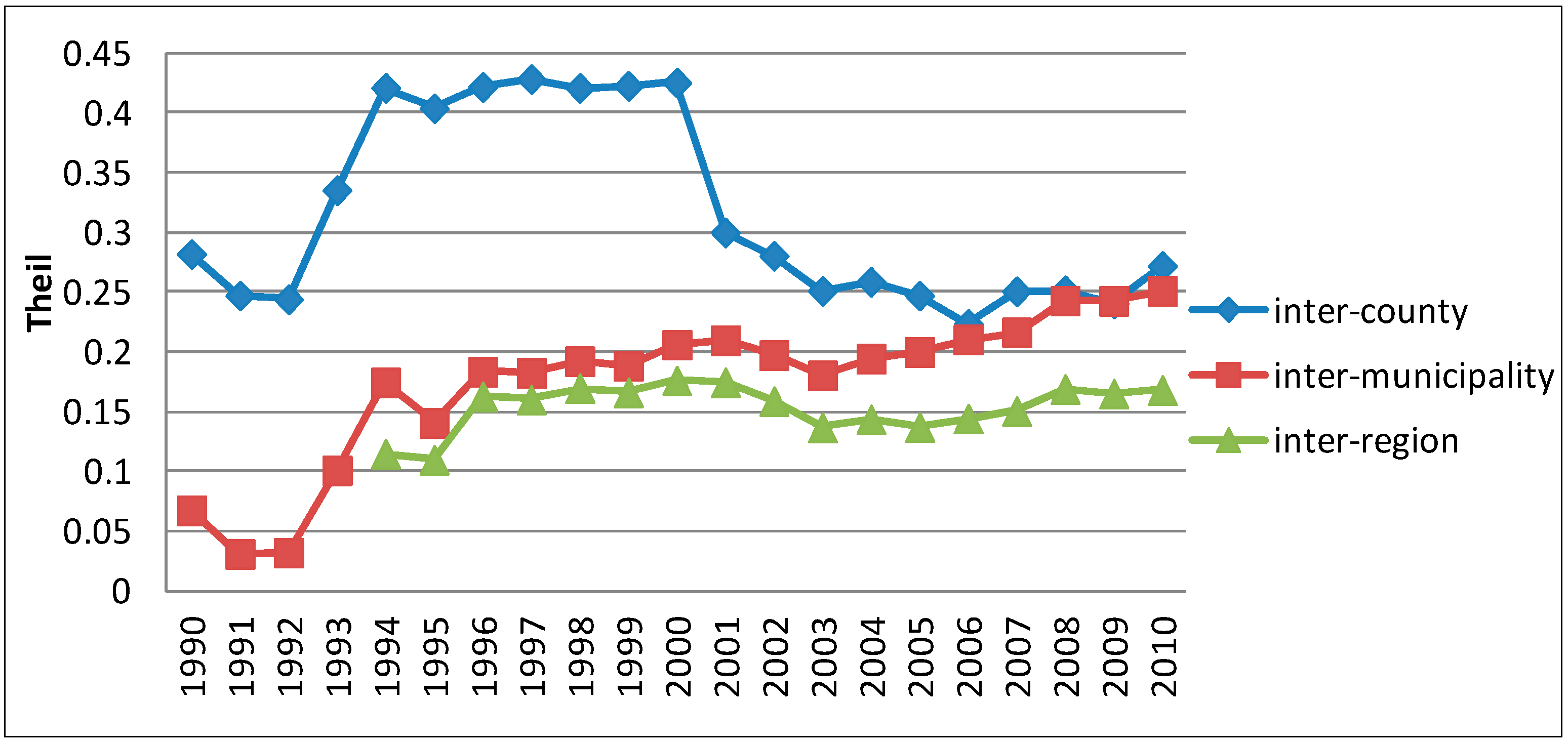
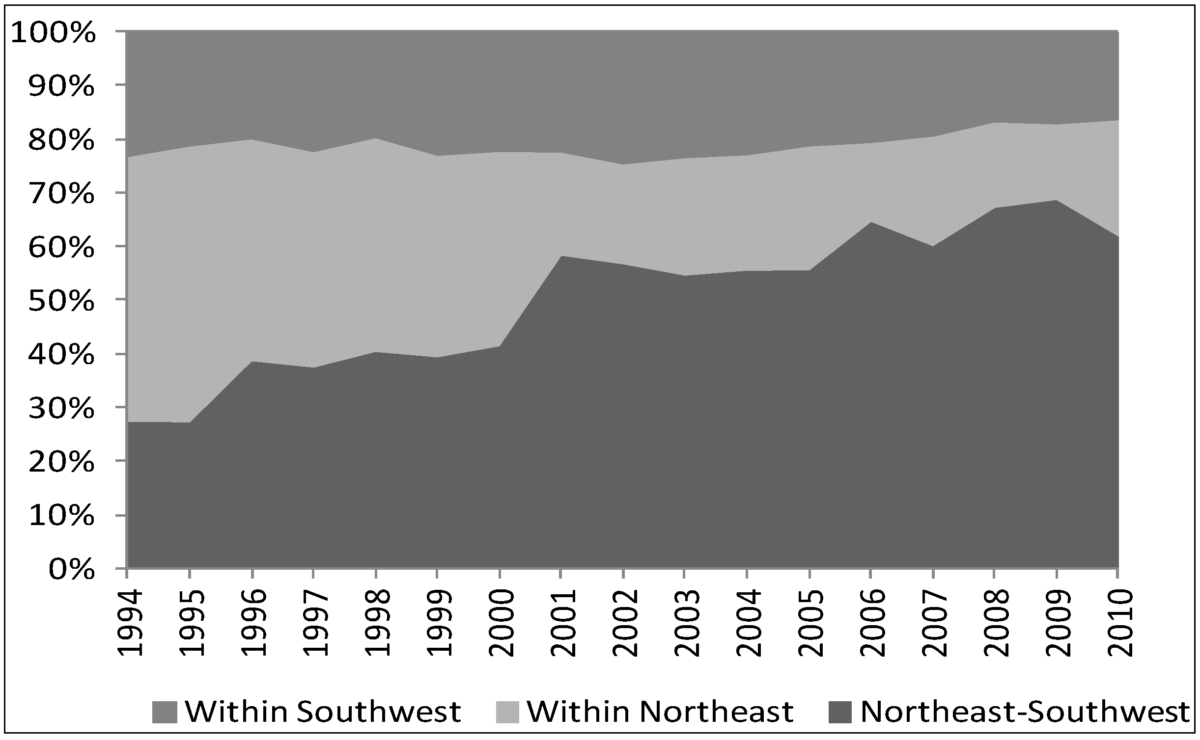
4.1. Multi-Scale Regional Inequality in Zhejiang

Figure 3 shows the dynamics of the regional inequality at three geographical scales in Zhejiang. The inter-county inequality fluctuates greatly, showing an evident inverted-U shaped pattern. The county-level Theil index decreased slightly between 1990 and 1992, and increased dramatically between 1992 and 1994, and was maintained at a higher level in the late 1990s, but showed a sharp decline in 2001 and reached a minimum value in 2006, and then began to rise between 2007 and 2010.
Figure 3. Regional inequalities at different scales in Zhejiang, 1990–2010: Theil index.
Sustainability 06 05763 g003
The inter-municipality inequality displays a more consistently upward trend, it decreased between 1990 and 1992, and increased dramatically between 1992 and 1994. In 1995, there was a slight decline. But between 1996 and 2001, the inter-municipality inequality began to rise again, and then displayed a limited degree of decline between 2001 and 2003, and then displayed an upward trend again from 2004 to 2010.
The evolution of the inter-region inequality between 1994 and 2010 is very similar to that of the inter-municipality inequality, but the difference is that the fluctuation of the inter-region inequality is smaller.
As is shown in Figure 3, the regional inequality has not shown persistent divergence or convergence trajectories while these changes are responsive to the different stages of reforms. First, from 1990 to 1992, the inter-county inequality and the inter-municipality inequality both decreased, this may be due to the decline of the state-owned enterprises (SOEs) and the development of private enterprises, the development speed of the leading regions supported by the SOEs slowed down, while the originally backward regions developed well due to the development of the private enterprises. Second, from 1992 to 1994, the inter-county inequality and inter-municipality inequality both increased dramatically, this was closely related to Dengxiaoping’s South China tour in Guangdong, which had stimulated a new round of “Socialist Marketization” reforms. Since then, Foreign Direct Investment (FDI) in Zhejiang increased dramatically, from 0.414 billion yuan in 1991 surging to 4.808 billion yuan in 1994 [16]. Northeast Zhejiang and the coastal areas attracted most of the investment because of its locational advantages, and rapid development in this area ensued, while the southwestern region of Zhejiang developed more slowly, leading to the sharp rise in regional inequality. Third, in 1995, there was a slightly declining inequality in the province, this was likely attributable to the double impact of national macro-control policies and a cyclic upturn in the economy. Fourth, from 2001 to 2003, the regional inequality of Zhejiang decreased everywhere, especially the inter-county inequality, which was closely linked with China’s entry into WTO. The economy of Zhejiang province is mainly a privately owned and foreign trade dependent economy. China’s entry into the WTO and resulting tariff reductions benefited those provinces which were dominated by the foreign trade based industries. Fifth, there has been a slightly rising inequality since 2006. This is because the benefits of China’s entry into WTO began to be felt, and after adapting to the new situation, the privately owned and foreign trade oriented businesses in Northeast Zhejiang and the Wentai region (Wenzhou and Taizhou), began to flourish, this resulted in the rise of the regional inequality in Zhejiang.
Figure 3 reflects a general trend of rising inequalities at the three geographical scales in Zhejiang during the past 20 years, and shows that the regional inequality in Zhejiang is sensitive to the geographical scales. The average values of the inter-county inequality, the inter-municipality inequality, and the interregional inequality in GDPPC are 0.32, 0.17, and 0.15, respectively. The regional inequality is more significant at finer spatial units. The inter-county inequality is significantly higher, probably because we take the municipal districts into consideration when selecting the counties as the geographical scale of research, while GDP per capita of municipal districts was significantly higher than that of other rural counties, such as the GDP per capita of the municipal district of Ningbo which is 137,572 yuan, while among other more rural counties of Ningbo the highest GDP per capita is only 73,037 yuan [1]. Comparing the evolution of regional inequality at the three geographical scales, we can find that regional inequalities at the three geographical scales almost show the same trend in the same years, but the magnitudes of the changes are very different, and the fluctuation of the inter-county inequality is much larger than that of inter-municipality inequality and interregional inequality. This is because the smaller geographical units are more susceptible to the changes of the macro-environment such as Reform and Opening Up, China’s entry into the WTO, and so on. An example of why this might be so is illustrated by the case of the closure of a single inefficient state owned industrial plant as a result of reform, this might impact a small area but not a larger population municipality or region.
In order to explore the relationship between the scale of the analysis and apparent inequality in Zhejiang, we decompose the overall inter-county inequality into the inequality between the Northeast Zhejiang and Southwest Zhejiang counties, the inequalities within the Northeast Zhejiang counties and the inequalities within the Southwest Zhejiang counties. As illustrated in Figure 4, in the composition of the overall inter-county inequality in Zhejiang, the contribution of the Northeast-Southwest inequality increased from 27.28% in 1990 to 61.78% in 2010, while the inequality within the Northeast Zhejiang counties decreased from 49.5% in 1994 to 21.88% in 2010, and the inequality within the Southwest Zhejiang slightly decreased from 23.25% in 1990 to 16.34% in 2010. This shows that the “Club Effect” with respect to regional inequality in Zhejiang is obvious, and that Zhejiang has formed a “developed club” (Northeast Zhejiang) and a “backward club” (Southwest Zhejiang). The overall inequality in Zhejiang is dominated by the inequality between the two “clubs”, and the contribution of the inequality within the clubs is very small, and the contribution of the inequality within the backward club is significantly smaller than the inequality within the developed club. The counties in Northeast Zhejiang has formed a developed club, because it is an important part of the Yangtze River Delta, located in the east coastal area of China and near Shanghai, its transportation access is good, and it can easily and effectively accept the radiation of industries out from Shanghai and Hangzhou, these factors have all contributed to the rapid development of Northeast Zhejiang’s economy. However, the counties in Southwest Zhejiang has formed a backward club, mainly because Southwest Zhejiang, especially the inland areas, has poor geographic location and poor infrastructure, and cannot easily get benefits from the radiation from Shanghai and Hangzhou, therefore it has experienced relatively slow development.
Figure 4. Theil decomposition of overall inter-county inequality in Zhejiang, 1994–2010.
Sustainability 06 05763 g004

4.2. Spatial Aggregation and the Dynamics of Inter-County Equality in Zhejiang Province

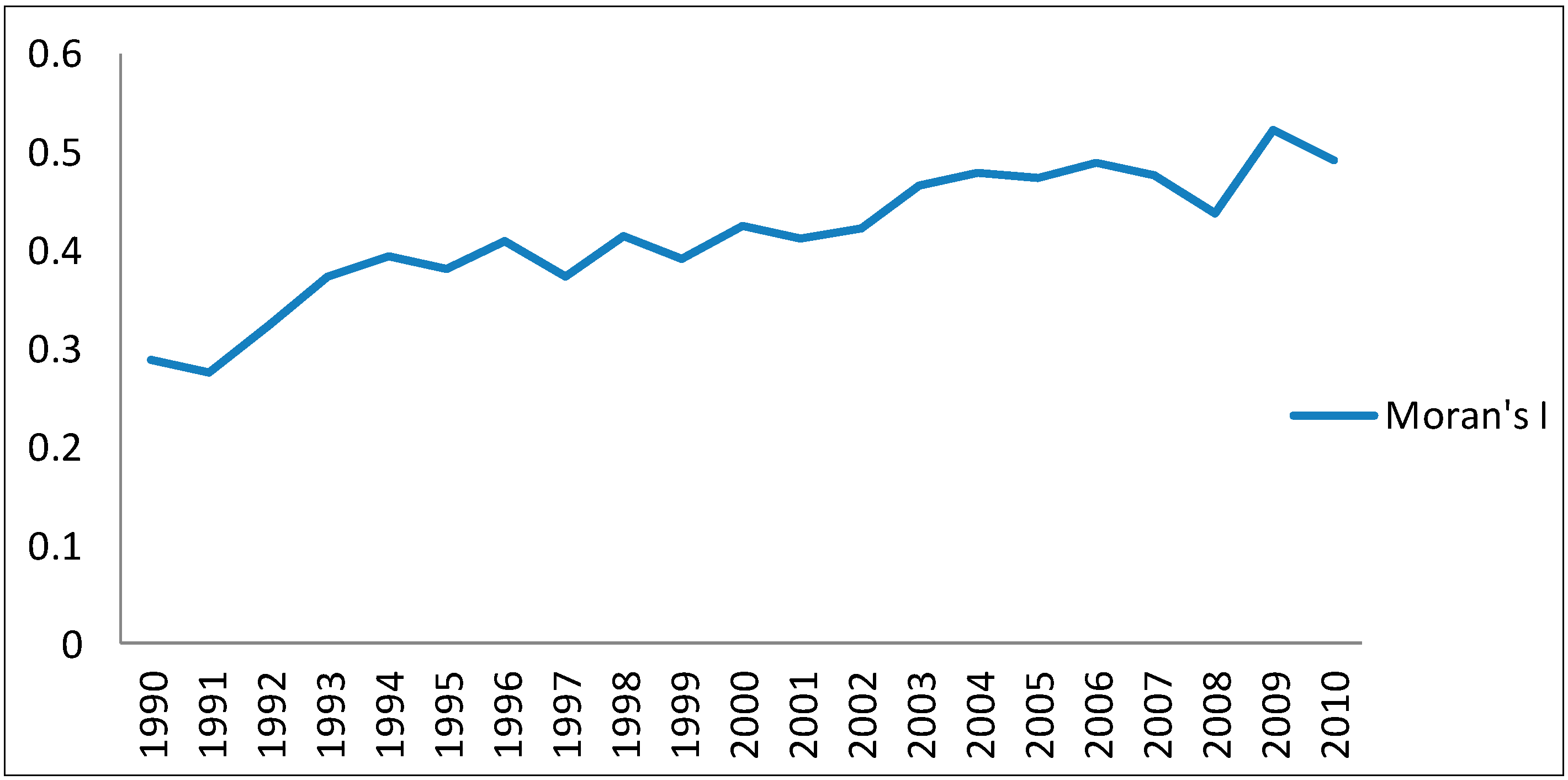
4.2.1. Global Spatial Autocorrelation

We computed the global Moran’s I to capture the overall tendency of development to exhibit geographical concentration on a regional basis in Zhejiang (Figure 5). A positive value indicates spatial clustering of similar values (high or low), and the higher the value is, the higher the degree of spatial aggregation is, and the smaller the overall inequality is. As illustrated in Figure 5, the values of global Moran’s I are all positive and increased from 0.289 in 1990 to 0.492 in 2010 and all are significant at the 0.01 level. This result implies that from 1990 to 2010, the counties, which have a similar level of economy development, cluster together, that the degree of spatial aggregation has been rising so the overall regional inequality has been decreasing. These are opposite to the results calculated by use of the Theil index. In fact, these two findings are not contradictory. The Theil index is a location-independent value, and simply reflects the degree of variation, while the Moran’s I is closely related to the location chosen and can reflect the degree of centralization or decentralization of a phenomenon. Zhejiang has formed a developed club (Counties in Northeast Zhejiang) and a backward club (Counties in Southwest Zhejiang) (Figure 4). As an important part of the Yangtze River Delta, Northeast Zhejiang’s economic development is rapid, while the economic development of Southwest Zhejiang has lagged behind, especially in inland areas, due to the disadvantages of its geographical isolation. With greater implementation of reforms and opening up the economy to exports and FDI, Northeast Zhejiang has formed an region with a spatial aggregation of developed counties, while the inland areas of Southwest Zhejiang have formed spatial aggregation of backward counties, and the inequality between the two regions has thus been constantly growing. The regional economic development in Zhejiang presents the characteristics that the inequality within Northeast Zhejiang and the inequality within Southwest Zhejiang have been shrinking, while the inequality between these two regions has been at the same time expanding.
Figure 5. Global Moran’s I of the county level GDP per capita in Zhejiang, 1990–2010.
Sustainability 06 05763 g005

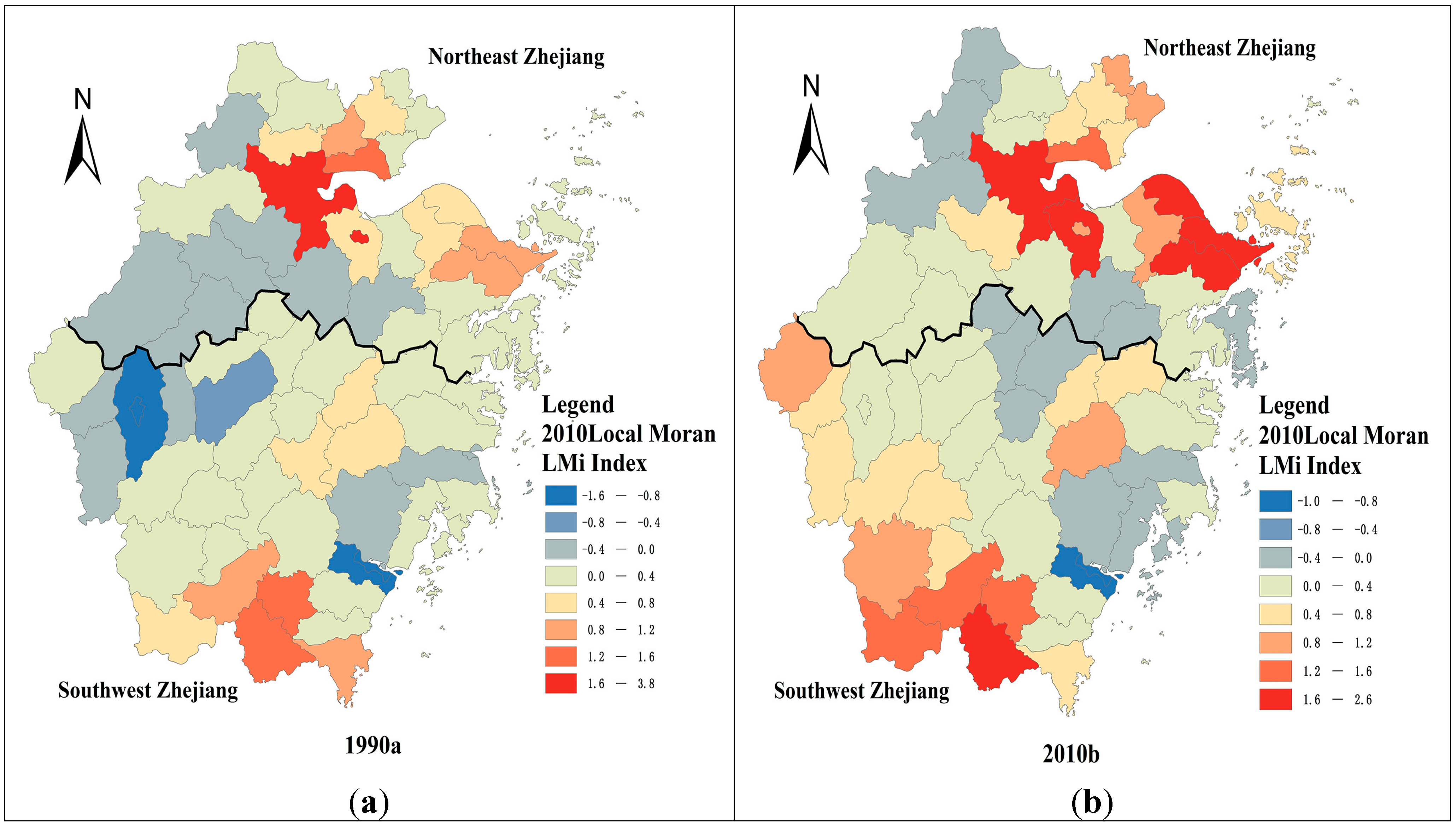
4.2.2. Local Spatial Aggregation

A Global Moran’s I can only provide insights into the global spatial autocorrelation of the regional economic development in Zhejiang, but it cannot provide insights into the spatial autocorrelation of each county within Zhejiang, so we then introduce the local Moran’s I into the analysis. The value of the local Moran’s I is larger than the global Moran’s I, indicating that the development of the study area is closer to that of its neighboring areas and the spatial aggregation is more obvious. Figure 6a shows that the spatial aggregation within Zhejiang was not obvious in 1990, the counties whose local Moran’s I is larger than 0.8 include Hangzhou municipal district, Haining, Tongxiang, Shaoxing municipal district, Ningbo municipal district, Jingning She Autonomous County, Wencheng, Taishun, Cangnan and so on. Combined with Figure 7a, we can see that Hangzhou municipal district, Haining, Tongxiang, Shaoxing municipal district and Ningbo municipal district form an area of spatial aggregation that is developed economically, while Jingning She Autonomous County, Wencheng, Taishun and Cangnan form an area of spatial aggregation that is economically backward. Figure 6b shows that the spatial aggregation within Zhejiang was very obvious in 2010, the counties whose local Moran’s I is larger than 0.8 include Hangzhou municipal district, Shaoxing County, Ningbo municipal district, Cixi, Shaoxing municipal district, Haining, Jiaxian, Pinghu, Yuyao, Xianju, Kaihua, Longquan, Qingyuan, Jingning She Autonomous County, Wencheng and Taishun. Combined with Figure 7c, we can see that Hangzhou municipal district, Shaoxing County, Ningbo municipal district, Cixi, Shaoxing municipal district, Haining, Jiaxian, Pinghu and Yuyao are areas that exhibit spatial aggregation and are economically developed, while Xianju, Kaihua, Longquan, Qingyuan, Jingning She Autonomous County, Wencheng and Taishun are areas that exhibit spatial aggregation and are economically backward.
By comparing Figure 6a with Figure 6b, we find that the spatial aggregation of Zhejiang in 2010 is much larger than it was in 1990, especially the spatial aggregation of the developed area of Northeast Zhejiang and the spatial aggregation of the backward area of Southwest Zhejiang, which reflects the fact that the inequality within Northeast Zhejiang and the inequality within Southwest Zhejiang have been shrinking, while the inequality between the two regions has been constantly growing. And this finding in turn provides an explanation for the “convergence” phenomenon of inequality exhibited in Zhejiang province.
Figure 6. Local Moran’s I of county level GDP per capita in Zhejiang, 1990, 2010.
Sustainability 06 05763 g006
Figure 7. Spatial patterns of regional development in Zhejiang province, 1990, 2000, and 2010.
Sustainability 06 05763 g007
P = poor; L = less developed; D = developed; R = rich.

4.3. The Spatial-Temporal Dynamics of County Level Regional Inequality in Zhejiang

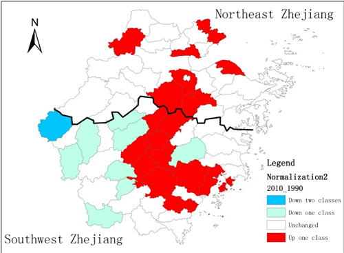
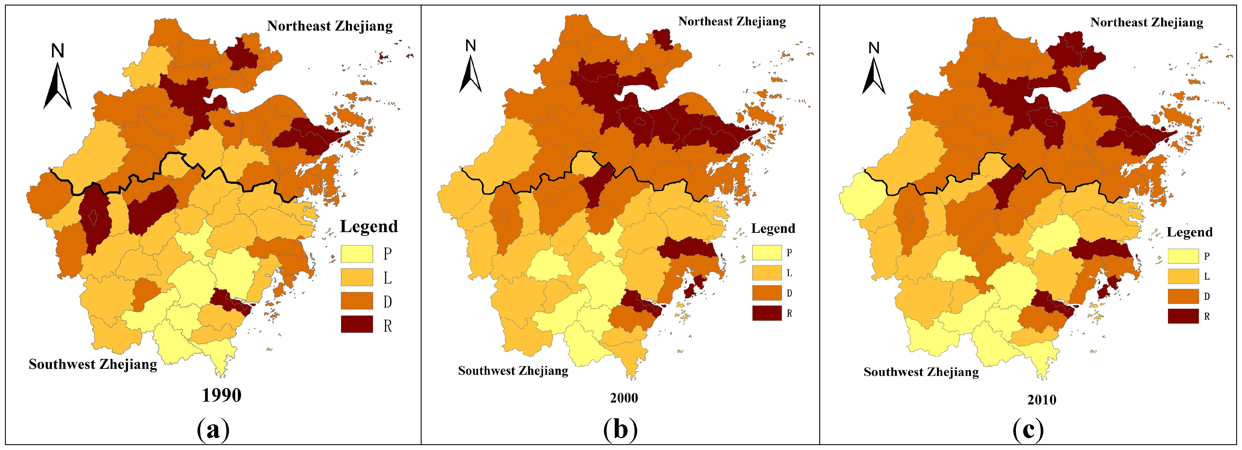
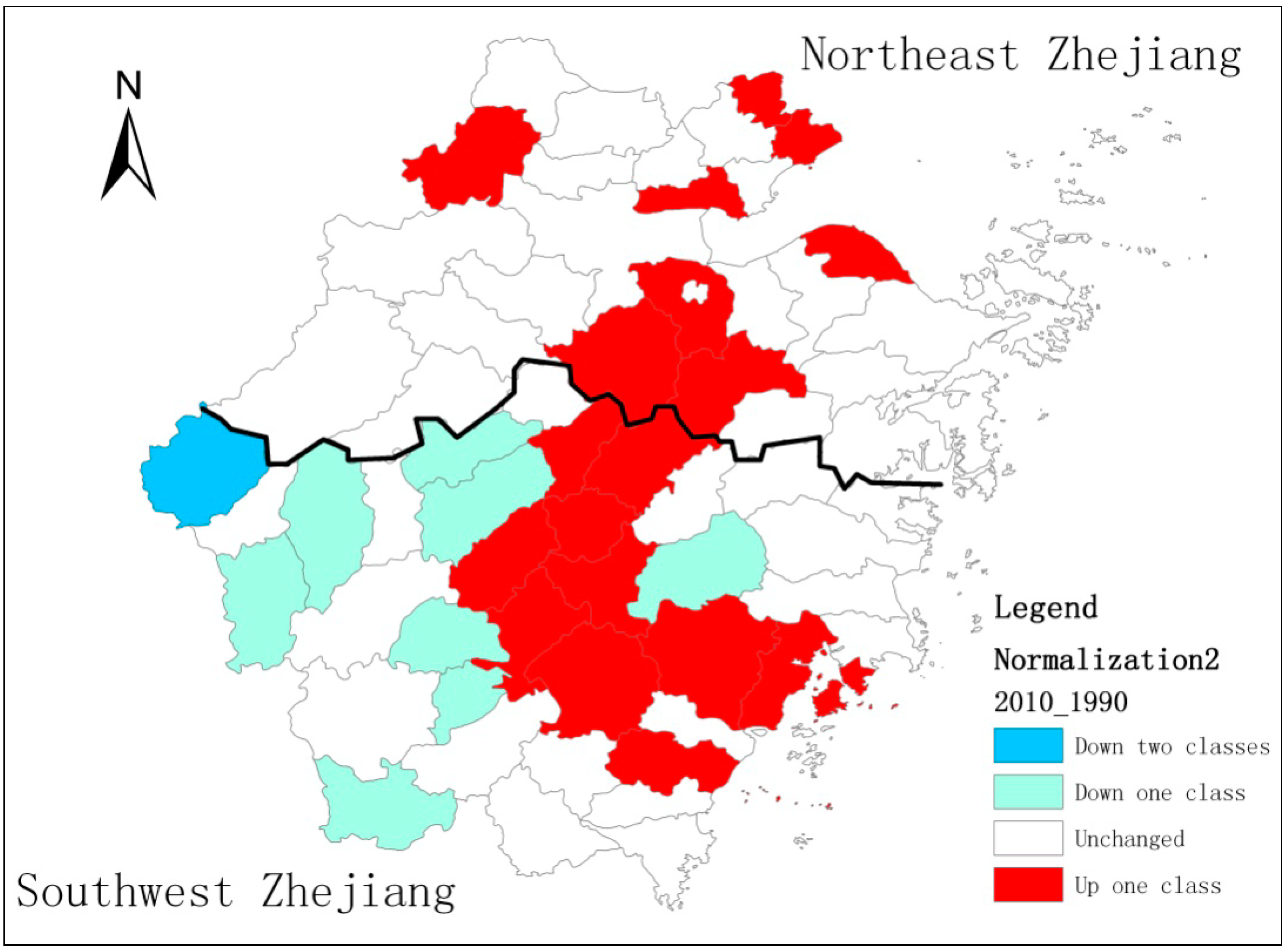
4.3.1. Spatial Patterns of Regional Development in Zhejiang Province

An analysis of the dynamic evolution over time of the spatial patterns of regional inequality can provide richer insights into the regional economic geography of Zhejiang. Figure 7 shows an obvious North-South divide of the regional economy in Zhejiang: most of the counties in the developed class and rich class are the counties in Northeast Zhejiang; most of the counties in the less developed class and poor class are the counties in Southwest Zhejiang; as the distance of a given county away from Northeast Zhejiang increases, counties are more likely to become poor. As illustrated in Figure 7a, in 1990, the spatial pattern of regional development in Zhejiang was relatively decentralized, the counties in the developed class and rich class were relatively dispersed, and there were counties in the rich class (Quzhou municipal district, Jinhua municipal district) in the inland areas of Southwest Zhejiang. In 2000, because of the regionally lopsided development of private enterprises, the statuses of some counties in the central Zhejiang has improved, such as Yiwu which moved upward from the developed class into the rich class and Zhuji, Shengzhou and Dongyang, which moved upward from the less developed class into the developed class. In comparison with the map in 1990, the North-South divide in Zhejiang in 2000 is more obvious, and the economic development of Zhejiang has shown an obvious “Club Effect”: Northeast Zhejiang (especially Hangzhou, Shaoxing, and Ningbo) have formed an obvious developed club, the coastal areas of Southwest Zhejiang have also formed an obvious developed club, while the inland areas of Southwest Zhejiang have formed an obvious backward club (Figure 7b). In 2010, the economic development of Zhejiang still exhibits obvious spatial aggregation and this “club effect” (Figure 7c). But in comparison with the map in 2000, in 2010, the counties in the poor class moved further to the south and inland areas. Several counties of Jiaxing such as Jiaxing municipal district, Jiashan, Pinghu, moved upward from the developed class to the rich class, mainly due to the advantages derived from their geographical proximity to Shanghai (Figure 7c).
Figure 8 shows the spatial pattern of county level GDP per capita changes between one class and another (a type transfer from developed to rich for example) in Zhejiang that took place from 1990 to 2010. There were 19 counties that moved upward in Zhejiang, including Jiashan, Anji, Shengzhou, Pinghu, Shaoxing, Cixi, Haining, Zhuji (all in Northeast Zhejiang) and Dongyang, Lishui municipal district, Yiwu, Leqing, Wuyi, Yongjia, Yongkang, Yuhuan, Ruian, Jinyun, Qingtian (all in Southwest Zhejiang). These counties in Southwest Zhejiang are mutually connected and affected by proximity to Northeast Zhejiang and coastal areas such as Wenzhou. There were nine counties who moved downward, including Xianju, Lanxi, Qingyuan, Songyang, Jiangshan, Quzhou municipal district, Jinhua municipal district, Yunhe and Kaihua. All of these counties are located in Southwest Zhejiang, and all are located in the inland areas, except Xianju. Kaihua moved downward by two classes, from the developed class in 1990 to the poor class in 2010. The fact that the counties who moved upward are mainly located in Northeast Zhejiang and coastal areas of Southwest Zhejiang and the counties who moved downward are mainly located in inland areas of Southwest Zhejiang, bolsters the finding that there has been a convergence among the members of the two disparate “clubs” that have developed in Zhejiang during the period of 1990–2010.
Figure 8. Spatial pattern of county level GDP per capita class changes (type transfers) in Zhejiang, 1990–2010.
Sustainability 06 05763 g008

4.3.2. Markov Chains Analysis of Regional Inequality

In this section, the dynamics that underlie regional inequality or the “long-run” properties of convergence or divergence across all 69 counties in Zhejiang are analyzed with the use of Markov chains.
Table 3 contains the transition probability matrices over the period between 1990 and 2010, as well as in the two sub-periods, the 1990s (socialist market system reform) and the 2000s (China’s accession into the WTO). The results of the Markov-chain analyses more clearly point out the system dynamics in Zhejiang’s regional development, which are sensitive to the different stages in the course of the reforms. First, the transition probabilities along the dialog are high. In other words, if a county falls into the specific class (rich, developed, less developed, and poor), the probability of its being in the same group in the next time period is at least 86.25%. Second, the transition probability between different groups is very low, and the highest transition probability is only 13.75% (Table 3). The results also show that it is very difficult for a county to leapfrog from poor to rich or from less developed to rich, and vice versa (this had a 0% probability of happening). Third, that the regional development regime in Zhejiang province exhibits a “club convergence” phenomenon: when a county ascends into the rich class, in the next year it has a 86.25% tendency of staying in the rich class and it has only a 13.75% tendency of moving downward, showing that the rich regions have a convergence trend; however, when a county falls into the poor class, it has a 91.23% tendency of remaining in the poor class and it has only an 8.77% tendency of moving upward, showing that it is very likely for poor areas to fall into a “poverty trap”.
Table 3. Markov-chain transitional matrices for county level GDP per capita, 1990–2010.
Transition ProbabilityPLDR
1990–2010
P(131)0.93130.068700
L(372)0.02690.92470.04840
D(609)00.02130.93760.0411
R(199)000.10050.8995
Ergodic distribution8.54%21.81%49.45%20.20%
1990–2000
P(57)0.91230.087700
L(181)0.02210.90610.07180
D(303)00.02970.92740.0429
R(80)000.13750.8625
Ergodic distribution5.69%22.60%54.65%17.05%
2001–2010
P(68)0.94120.058800
L(170)0.03530.93530.02940
D(274)00.01460.94890.0365
R(109)000.08260.9174
Ergodic distribution13.32%22.20%44.72%19.76%
P = poor; L = less developed; D = developed; R = rich; the numbers in the parentheses are total numbers of transitions.
From the point of view of frequency, in the 1990s, the numbers of counties, which for the first time fell into the poor class and ascended into the rich class were 57 and 80 respectively, while in the 2000s, the two numbers increased to 68 and 109 respectively. This shows that more counties are becoming relatively rich than relatively poor but that more counties are both becoming relatively richer and relatively poorer, this tends to exacerbate issues of inequality.

4.3.3. Spatial Markov Chains of Regional Inequality

The traditional Markov approach can be used for the analysis of the evolution of regional convergence (or divergence), but as the method sees the different regions as “islands” ignoring the spatial interaction between regions, it can’t reveal the spatial characteristics of the evolution of regional economies [6,17,28]. Thus, to fully understand these dynamic uses of spatial Markov chain analysis is called for. The results of the spatial Markov-chain analysis are shown in Table 4. They provide more details about the possible association between the direction and probability of transitions and the neighborhood context. First, for the poorest counties, the probability of an upward transition is affected by the economic development of neighboring counties. Firstly as shown in Table 3, the poorest counties in general have a 6.87% tendency to move upward. However, if a poor county is surrounded by other poor counties, the tendency of it to move upward drops to 3.8%. Meanwhile, if the neighbors of a poor county are relatively richer counties, such as less developed rather than poor counties, the tendency of a poor county to move upward increases to 11.54% (Table 4). Secondly, another finding is that the less developed counties have a 2.69% tendency to move downward regardless of the status of neighboring counties. However, if the neighbor of a less developed county is poor, that county has higher probability of moving downward (3.12%). Meanwhile, if the neighbors of a less developed county are developed counties, its tendency of moving downward drops to 1.76%. For less developed counties the tendency of it moving upward increases from 4.84% to 13.33% regardless of its neighborhood status. Thirdly, for a county in the developed class, it in general has a 2.13% tendency of moving downward regardless of its neighborhood status. However, if its neighbor is a less developed county, it has a higher chance (13.04%) of becoming a less developed county. Meanwhile, if its neighbor is rich, the tendency of moving upward from the developed class to the rich class increases from 4.11% regardless of its neighborhood status (Table 3) to 6.02% (Table 4). Fourthly, the comparison of Table 3 and Table 4 shows that the neighborhood effect doesn’t significantly apply to the rich counties. For the rich counties, their developments are less influenced by their neighbors, but more by their own development conditions (such as the geographical location) and macro environment (such as China’s entry into the WTO). In our future study, the Markov process could be conditioned on each region’s trade openness. In addition, the spatial Markov-chain provides a spatial explanation for the “club convergence” phenomenon of regional development in Zhejiang. In general, if a county is adjacent to poorer counties, it will be negatively affected, however, if its neighbors are richer counties, the probability of its moving upward will increase.
The spatial Markov-chain reveals that the economic development of a county is affected by the economic development of its neighboring counties. This is proved by analysis of the spatial pattern of county level GDP per capita type transfer in Zhejiang between 1990 and 2010 (Figure 8). It can be observed that the counties, which have moved upward are always adjacent to the relatively richer regions, these counties in Northeast Zhejiang are adjacent to Hangzhou, Ningbo or Shanghai. The counties in Southwest Zhejiang that have moved up are all adjacent to Wenzhou or Northeast Zhejiang; however, the counties which have moved downward are always adjacent to the relatively poorer regions, and all of these counties are located in Southwest Zhejiang, especially in the inland areas of Southwest Zhejiang, and the poor counties and less developed counties are almost all located in Southwest Zhejiang. This indicates that Southwest Zhejiang, especially its inland areas, have fallen into a “poverty trap”.
Table 4. Spatial Markov-chain transition matrix for county level GDP per capita in Zhejiang, 1990–2010.
2010
Spatial lag1990PLDR
PP0.9620.03800
L0.03120.91670.05210
D00.0180.94590.036
R000.0750.925
LP0.88460.115400
L0.02870.95220.01910
D00.13040.86960
R0000
DP0000
L0.01670.850.13330
D00.01250.94670.0408
R000.09520.9048
RP0000
L00.85710.14290
D00.00750.93230.0602
R000.12990.8701
P = poor; L = less developed; D = developed; R = rich.

4.3.4. The Trend of Spatial-Temporal Dynamics of Regional Inequality in Zhejiang

Spatial Markov-chain analysis and the spatial pattern of county level GDP per capita type transfer between 1990 and 2010 (Figure 8) further reveal the potential evolution of regional inequality in Zhejiang. First, the developed aggregation in Northeast Zhejiang will likely intensify, and the number of rich counties will increase. Haiyan and Tongxiang may move upward from the developed class to the rich class under the influence of proximity to Shanghai and Hangzhou, and Shangyu and Yuyao may also move upward from the developed class to the rich class under the influence of proximity to Hangzhou and Ningbo. Second, the coastal areas of Southwest Zhejiang will have a greater opportunity for economic development, Yongjia may be influenced by Wenzhou’s municipal district, Yueqing and Taizhou municipal district and it may move upward from the less developed class to the developed class, and Xianju may move upward from the poor class to the less developed class under the influence of its neighboring counties which are in higher classes. Meanwhile, the inland areas of Southwest Zhejiang will continue to be relatively poor, and the number of poor counties will be likely to increase. Longquan and Yunhe may move downward from the less developed class to the poor class. Third, analysis of the regional inequality in Zhejiang will likely reveal that the inequality within Northeast Zhejiang will decline, while the inequality within Southwest Zhejiang may rise and the inequality between Northeast and Southwest will be further aggravated. Meanwhile, the spatial aggregation phenomenon in Zhejiang will be intensified.

5. Conclusions

This paper analyzes the regional equality in one of China’s most developed provinces, Zhejiang. It confirms the applicability of a multi-scale framework at the intra-provincial level. We find that regional inequality in Zhejiang is sensitive to the choice of geographical scales: the inter-county inequality shows an inverted-U shape pattern, the inter-municipality inequality displays a more consistently upward trend, and the evolution of the interregional inequality is relatively stable over time. This paper emphasizes the distinctive distributional dynamics at the different stages of economic reform from an evolutionary perspective. The analysis of the Theil decomposition of overall inter-county inequality reveals that the contribution of the inequality within Northeast Zhejiang and within Southwest Zhejiang has been constantly declining, while the contribution of the inequality between Northeast Zhejiang and Southwest Zhejiang has been constantly rising. Zhejiang province has formed a club of developed counties (in Northeast Zhejiang) and a club of backward counties (in Southwest Zhejiang).
The results of analysis of local Moran’s I show that Northeast Zhejiang has formed a rich cluster and Southwest Zhejiang has formed a poor cluster. Traditional Markov chain analysis shows that if a county falls or ascends into a specific class (rich, developed, less developed, and poor), the probability of its being in the same group is very high and the transition probability between different groups is very low. It also explains the “club convergence” phenomenon of economic development in Zhejiang.
Despite the recent efforts to strengthen the study of intra-provincial inequality and incorporating GIS-based spatial analysis [4,19,20,21,22,23], regional inequality in provincial China needs to be further studied and the capacities of GIS have yet to be fully realized. As a descriptive approach, exploratory spatial data analysis methods have the limitation in revealing or verifying the mechanism underlying the dramatic transition. Hence, the driving forces influencing regional inequality in Zhejiang will be further analyzed in a follow-up study.

Acknowledgments

This work has been supported by the Humanities and Social Sciences Planning Fund of the Chinese Ministry of Education (13YJA630120), Key Project of Chinese Ministry of Education (No.13JJD790008), the National Natural Science Foundation of China (41329001), the Fundamental Research Funds for the Central Universities and the Policy Simulation Lab at Zhejiang University.

Author Contributions

Wenze Yue designed research and wrote the paper, Yuntang Zhang performed research, analyzed the data and wrote the paper, Xinyue Ye co-designed research and extensively updated the paper, Yeqing Cheng did part of the literature review and checked the statistical results, Mark R. Leipnik edited the paper. All authors read and approved the final manuscript.

Conflicts of Interest

The authors declare no conflict of interest.

References

  1. Wei, Y.D.; Ye, X. Beyond convergence: Space, scale, and regional inequality in China. J. Econ. Soc. Geogr. 2009, 100, 59–80. [Google Scholar]
  2. Wei, Y.D.; Yu, D.; Chen, X. Scale, agglomeration, and regional inequality in provincial China. J. Econ. Soc. Geogr. 2011, 102, 406–425. [Google Scholar]
  3. Fan, C.C.; Sun, M. Regional inequality in China, 1978–2006. Eurasian Geogr. Econ. 2008, 49, 1–18. [Google Scholar] [CrossRef]
  4. Yu, D.; Wei, Y.D. Analyzing regional inequality in post-Mao China in a GIS Environment. Geogr. Econ. 2003, 44, 514–534. [Google Scholar] [CrossRef]
  5. National Bureau of Statistics of China. China Statistical Yearbook, 2011; China Statistics Press: Beijing, China, 2011. [Google Scholar]
  6. United Nations Development Program (UNDP). Human Development Report 2014; United Nations Development Program: New York, NY, USA, 2014. [Google Scholar]
  7. Wei, Y.D.; Ye, X. Regional inequality in China: A case study of Zhejiang Province. J. Econ. Soc. Geogr. 2004, 95, 44–60. [Google Scholar]
  8. Barro, R.J.; Sala-I-Martin, X. Convergence across states and regions. Brook. Papers Econ. Act. 1991, 22, 107–182. [Google Scholar]
  9. Barro, R.J.; Sala-i-Martin, X. Convergence. J. Political Econ. 1992, 100, 223–251. [Google Scholar] [CrossRef]
  10. Li, Y.; Wei, Y.D. The spatial-temporal hierarchy of regional inequality of China. Appl. Geogr. 2010, 30, 303–316. [Google Scholar] [CrossRef]
  11. Weng, Q. Local impacts of the post-Mao development strategy: The case of the Zhujiang Delta, southern China. Int. J. Urban Reg. Res. 1998, 22, 425–442. [Google Scholar] [CrossRef]
  12. Wei, Y.D. Regional development in China: Transitional institutions, embedded globalization, and hybrid economies. Eurasian Geogr. Econ. 2007, 48, 16–36. [Google Scholar] [CrossRef]
  13. Ye, H.; Chen, X. The analysis of the regional economic inequality in Zhejiang in recent 16 years. Explor. Econ. Probl. 2008, 2, 59–65. [Google Scholar]
  14. Luo, D. The analysis of regional inequality of economic development in Zhejiang. Econ. Res. Guide 2009, 42, 102–103. [Google Scholar]
  15. Rey, S.J.; Murray, A.T.; Anselin, L. Visualizing regional income distribution dynamics. Lett. Spat. Resour. Sci. 2011, 4, 81–90. [Google Scholar] [CrossRef]
  16. Rey, S.J.; Anselin, L. PySAL: A Python library of spatial analytical methods. In Handbook of Applied Spatial Analysis; Fischer, M., Getis, A., Eds.; Springer: Berlin/Heidelberg, Germany, 2007; pp. 175–193. [Google Scholar]
  17. Anselin, L.; Syabri, I.; Kho, Y. GeoDa: An introduction to spatial data analysis. Geogr. Anal. 2006, 38, 5–22. [Google Scholar] [CrossRef]
  18. Celebioglu, F.; Dall’erba, S. Spatial disparities across the regions of Turkey: An exploratory spatial data analysis. Anna. Reg. Sci. 2010, 45, 379–400. [Google Scholar] [CrossRef]
  19. Le Gallo, J.; Ertur, C.  Exploratory spatial data analysis of the distribution of regional per capita GDP in Europe, 1980–1995. Papers Reg. Sci. 2003, 82, 175–201. [Google Scholar]
  20. Rey, S.J.; Janikas, M. 2005 Regional convergence, inequality, and space. J. Econ. Geogr. 2005, 5, 155–176. [Google Scholar] [CrossRef]
  21. Rey, S.J. Spatial empirics for economic growth and convergence. Geogr. Anal. 2001, 33, 195–214. [Google Scholar] [CrossRef]
  22. Rey, S.J. Rank-based Markov chains for regional income distribution dynamics. J. Geogr. Syst. 2014, 16, 115–137. [Google Scholar] [CrossRef]
  23. Gallo, J. Space-time analysis of GDP disparities among European regions: A Markov chains approach. Int. Reg. Sci. Rev. 2004, 27, 138–163. [Google Scholar] [CrossRef]
  24. Rodríguez-Pose, A.; Vassilis, T. Mapping regional personal income distribution in Western Europe: Income per capita and inequality. Financ. Uver-Czech J. Econ. Financ. 2009, 59, 41–70. [Google Scholar]
  25. Rodríguez-Pose, A.; Vassilis, T. Mapping the European regional educational distribution. Eur. Urban Reg. Stud. 2011, 18, 358–374. [Google Scholar]
  26. Zhejiang Province Statistics Bureau. Zhejiang Statistical Yearbook, 2011; China Statistics Press: Beijing, China, 2011. [Google Scholar]
  27. Ye, X.; Wei, Y.D. Geospatial analysis of regional development in China: The case of Zhejiang Province and the Wenzhou model. Eurasian Geogr. Econ. 2005, 46, 445–464. [Google Scholar] [CrossRef]
  28. Rey, S.J. Show me the code: Spatial analysis and open source. J. Geogr. Syst. 2009, 11, 191–207. [Google Scholar] [CrossRef] [Green Version]
  29. Anselin, L. Local indicators of spatial association-LISA. Geogr. Anal. 1995, 27, 93–115. [Google Scholar] [CrossRef]

