Article

Retail Services and Pricing Decisions in a Closed-Loop Supply Chain with Remanufacturing

School of Management, Huazhong University of Science and Technology, Wuhan 430074, China
*
Author to whom correspondence should be addressed.
Sustainability 2015, 7(3), 2373-2396; https://doi.org/10.3390/su7032373
Submission received: 30 October 2014 / Accepted: 24 December 2014 / Published: 27 February 2015
(This article belongs to the Special Issue Sustainable Business and Development II)

Abstract

:
Environmental and social responsibilities have led many manufacturers to used products recovery. Meanwhile, many manufacturers nowadays sell products via indirect retailer channels and direct Internet channels. This paper models a dual-channel closed-loop supply chain to improve the sustainability of products. We apply the two-stage optimization technique and the Nash game to examine the impacts of the retail services and the degree of customer loyalty to the retail channel on the pricing of players in a centralized and a decentralized dual-channel supply chain. Our results show that the retail services have a great impact on the manufacturer and the retailer’s pricing strategies. We also compare the differences of pricing strategies between a centralized and a decentralized dual-channel supply chain and suggest the optimal retail services and pricing decisions for the players in the supply chain.

1. Introduction

Due to environmental and social responsibilities, people realize that profits and profitability are not the only elements for companies. For a responsible company, the future of the planet and the people are important. Legislation introduced in North America, Europe and Asia motivates many corporations to take measures on environmental protection. For example, the European Union legislates that all producers and retailers implement systems allowing any end users to return a product. Some top suppliers, such as Xerox, ReCellular, IBM and Dell, are participating in collecting used products from third party collectors and users. The sustainable effort-related factors also have an impact on customer selection decisions [1]; therefore, supply chain management tends to be energy saving and less material consuming. A sustainable product program, which upgrades the classical kinds of supply chains, is set up for environmental improvement and the health and safety of the employees and the sustainability of the whole society [2]. This kind of reverse supply chain is also beneficial to save production costs, generate revenue and satisfy the demand of customers [3].
On the other hand, with the rapid development of the Internet, the supply chain system is no longer a single traditional channel, and many manufacturers set up direct channel to sell products online [4]. This new supply system, in which a manufacturer sells products not only directly to customers, but also through its retailers, is called the dual-channel. In a dual-channel distribution setting, customers can buy the same products from both a manufacturer and its retailer. This dual-channel often provides more shopping choices and price savings for customers. As a result, customers are more likely to purchase products and services via the direct sale channel.
In recent years, dual-channel supply chain has intrigued both researchers and practitioners. Chiang et al. [5] considered a manufacturer and its independent retailer in a price setting game and found that direct marketing improved overall profitability. Tsay and Agrawal [6] showed that direct sales would be beneficial to the manufacturer and its reseller if there were the associated adjustment of the manufacturer’s pricing. Seifert et al. [7] studied the problem of retailer sales channels and found that retailers would gain more profits from direct sales. Cai [8] showed that the performances of the supplier and retailer depended on demand, channel operational costs and channel substitutability.
The issue of retail services in the supply chain received some attention in the management press. Chen et al. [9] studied the services competition between the traditional channel and direct channel from the customers’ perspective and found that optimal dual-channel strategies depended on the channel environment. Yan and Pei [10] analyzed the effect of improved retail services, which resulted in a lower wholesale price, a higher sales volume and reducing the channel conflict in dual-channel competition. Meanwhile, Dumrongsiri et al. [11] found that both parties in a dual-channel supply chain profited when the level of a retailer’s services increased. Hu and Li [12] applied stochastic comparison method to analyze the retail services for the dual-channel. Their results showed that the manufacturer benefited from increased demand. Yao and Liu [13] modeled the price competition of Bertrand and Stackelberg and showed that a dual-channel supply system promoted not only competitive pricing and payoffs, but also cost effective retail services. Hall and Porteus [14] investigated a model with two capacitated firms, and found that those demands depended on the customer service levels. Similarly, Bernstein and Federgruen [15] found that in retail service competition, the retailer’s price increased in its own level of retail services, but decreased in the competitor’s level of retail services. Boyaci and Gallego [16] modeled a customer service competition game and showed that in a coordinated setting, all of the players in the supply chain maximized supply chain profits by coordinating their service and inventory policy decisions.
Meanwhile, a number of papers examined the pricing strategy in the supply chain. Cai et al. [17] argued that price discount contracts and a consistent pricing scheme improved the performance of the dual-channel supply chain. Kurata et al. [18] focused on pricing policies under brand competition and channel competition. They modeled a Nash pricing game and showed that the dynamic pricing strategy was helpful to coordinate the supply chain. Geng and Mallik [19] considered the coordination in a dual-channel supply chain and showed that the profit of the chain would increase with a combination contract of reverse revenue sharing and a fixed franchise fee. Chiang [20] explored a combination mechanism of a holding cost subsidy contract and a retail revenue sharing contract to coordinate the dual-channel supply chain. Boyaci [21] determined that simple contacts would not be able to coordinate the multiple-channel supply chain unless the retailer gained extra sales.
As mentioned before, many researchers have focused on product recovery. Majumder and Groenevelt [22] modeled a two-period remanufacturing game and studied the remanufacturing cost in the competition. Teunter and Flapper [23] studied the problem about recycling products of multiple quality classes, which was based on certain and uncertain demands, and found the optimal recycling and remanufacturing strategy. Savaskan et al. [24] showed that a manufacturer usually collects used products directly by itself, through its retailer or from a third party. They analyzed used product return rates, retail prices and manufacturer’s and retailer’s profits in the three kinds of recycling channels. The results showed that the retailer doing the collecting was the best recycling choice in a closed-loop supply chain. However, Gu et al. [25] indicated that the manufacturer doing the collecting was the optimal reverse strategy by comparing the pricing and the profits in the same three channels. Savaskan and Van Wassenhove [26] introduced a manufacturer and two competing retailers to the reverse channels. They found that the manufacturer engaged in direct reverse channels when the competition between the retailers was drastic. Otherwise, it would choose indirect channels to recover used products. Recent studies also showed much interest in the closed-loop supply chain. Qiang et al. [27] investigated a CLSC (closed-loop supply chain) network model, where the manufacturer collected recycled products in the direct channel. They showed that neither manufactured products nor remanufactured products had a significant effect on the retailer and consumer if the two kinds of products were comparable in function and quality. Ozkir and Basligil [28] also modeled a CLSC network in which there were three different recovery methods (material recovery, component recovery and product recovery) and found that a better CLSC strategy was determined by the quality of the returned products. Neto et al. [29] argued that bulk recycling was not a good option in CLSC. Georgiadis and Athanasiou [30] proposed flexible policies to coordinate CLSC with remanufacturing. Chen and Bell [31] showed that the retailers profited from different returns policies, which also had an impact on the retailers’ pricing and ordering decisions.
The studies in recent years mainly have focused on pricing strategy and product recovery in the reverse supply chain, while retail services seemed to be overlooked. We find that the above studies have made important contributions to the dual-channel closed-loop chain management, and we benefit a great deal from them. We think some inadequacies should be focused on. For instance, there is little research on how retail services and pricing are affected by other factors, such as the degree of customer loyalty to the retail channel in the supply chain. Meanwhile, many companies start to recover used products through their retailers or by themselves, and the return rate of used products is also an important factor. This paper contributes our perspective to the pricing strategy and retail services in a closed-loop supply chain. To fill the gap, we analyze the impacts of both retail services and the degree of customer loyalty to the retail channel on the pricing of players in a centralized and a decentralized dual-channel supply chain.
More specifically, we address the following research questions:
(1)
How are the pricing strategy and profits of the players in the supply chain affected by the retail services and the degree of customer loyalty to the retail channel?
(2)
What are the differences of the retail service decision and pricing strategy between a centralized and a decentralized dual-channel supply chain, respectively?
This paper is organized as follows. Section 2 introduces the notations and assumptions for the manufacturer and the retailer in the model. In Section 3 and Section 4, we examine the level of retail services, the return rate, the degree of customer loyalty to the retail channel and the pricing strategy in both a centralized and a decentralized dual-channel supply chain. In Section 5, we show the results of numerical examples carried out to examine the impacts of the retail services and the degree of customer loyalty to the retail channel on the pricing strategy of players in the two settings and the return rate. We conclude with key results and some managerial implications for future research in Section 6.

2. Model Notations and Assumptions

2.1. Notations

We use the following notations in this paper: c m is the unit manufacturing cost of new products, and c r is the unit remanufacturing cost of used products; w is the wholesale price of new/remanufactured products; p r is the retail price of products; p d is the direct sale price of products; D r is the consumer demand from the retail channel; D d is the consumer demand from the direct sale channel; a is the total demand in the market; s denotes the level of the retail services/the retail services cost; and θ denotes the degree of customer loyalty to the retail channel. The superscripts “c” and “d” mean the parameters corresponding to the centralized and decentralized system, respectively.

2.2. Assumptions

Assumption 1.
The unit manufacturing cost of new products is greater than that of used products, i.e., c m > c r .
Let Δ = c m c r , which denotes the unit cost savings from remanufacturing used products. We assume that the unit remanufacturing cost of used products is the same for all remanufactured products. This assumption about cost structures is based on the literature [24].
Then, we obtain the average unit cost of products:
c ¯ = ( 1 τ ) c m + τ c r = c m Δ τ
where τ denotes the used products’ return rate. As mentioned in previous literature [10], we have the cost of the retail services:
c ( s ) = η s 2 / 2
Assumption 2.
C τ 2 denotes the return cost of the retailer, where C is a scaling parameter, and 0 τ 1 .
τ means the customers’ motion to return the used products in the reverse channel. Similar forms also have been found to characterize product awareness and consumer retention in the advertising response models and to characterize product collection effort in remanufacturing [32]. A similar form of the return cost of the retailer has been used in [24].
Assumption 3.
The unit buyback price b is no larger than Δ , i.e., 0 < b Δ .
We assume that the remanufacturing is economically viable, which has been widely mentioned in the literature [32]. The process of remanufacturing used products is profitable for the manufacturer. The retailer can get a fixed payment b from the manufacturer, which does not influence the demand in the market, and the customer who returns used products is not paid by the retailer.
Assumption 4.
The wholesale price is higher than the cost of retail services and lower than both the retail price and the direct sale price, i.e., c < w < p r , p d .
Following Hua et al. [33], we assume that D r , D d 0 , then we have:
c ¯ < w < p r E s + A
c ¯ < w < p m F s + B
where:
A = θ a b 1 + ( 1 θ ) a b 2 b 1 2 b 2 2 ;   B = θ a b 2 + ( 1 θ ) a b 1 b 1 2 b 2 2 ;   E = β r b 1 β m b 2 b 1 2 b 2 2 ;   F = β r b 2 β m b 1 b 1 2 b 2 2
Assumption 5.
The retail price sensitivity of the demand is greater than the direct sale price sensitivity of the demand, i.e., β r > β m the retail service sensitivity of the demand in the retail channel is greater than that in the direct channel, i.e., b 1 > b 2 .
Based on Dan et al. [34], let:
μ = ( β r β m / β r ) ( b 1 b 2 / b 1 )
which denotes the ratio of the relative increase of the demand in the two channels due to an increase in retail services and the direct sale price.
Assumption 6.
The quality and price of the remanufactured products are the same as those of the new products.
In remanufacturing models, such as Savaskan and Van Wassenhove [26], the remanufactured products and new products are assumed to be sold at the same price.
Assumption 7.
All of the supply chain players have access to the same information.
The full information assumption is widely used in previous research [24,32]. We assume a symmetric relationship between the manufacturer and the retailer. It is assumed that the manufacturer and the retailer independently and simultaneously maximize their profits with respect to any possible strategies set by the other member in the supply chain. To control for inefficiencies and risk-sharing issues [35], we assume that all of the players in the supply chain can get access to the same information.
From the above notations and assumptions, the consumer demand functions from the retail channel and the direct channel are given by:
D r = θ a b 1 p r + b 2 p d + β r s
D d = ( 1 θ ) a b 1 p d + b 2 p r β m s
The retailer’s profit function and the manufacturer’s profit function are given by:
Π r = ( p r w ) + D r + b τ ( D r + D d ) C τ 2 η s 2 / 2
Π m = ( w c ¯ ) D r + ( p d c ¯ ) D d b τ ( D r + D d )

3. Analysis of the Centralized Dual-Channel Supply Chain

This supply chain model is centralized, so there is only a single decision maker. We consider the whole chain profits as best, and then, we have the profit of the centralized dual-channel supply chain:
c = r + m
Substituting Equations (1)–(6) into Equation (7), we obtain:
c = ( p r c m + Δ τ ) ( θ a b 1 p r + b 2 p d + β r s ) + ( p d c m + Δ τ ) [ ( 1 θ ) a b 1 p d + b 2 p r β m s ] C τ 2 1 2 η s 2
Proposition 1.
The dual-channel profit c is strictly jointly concave in p r , p d and τ , but not jointly concave in p r , p d , τ and s .
All of the proofs of the propositions in this section are given in the Appendix. Proposition 1 indicates that we cannot get the optimal values of p r , p d , τ and s just from the first-order conditions. Following Dan et al. [34], we can apply the two-stage optimization technique to derive them, because c has a unique optimal solution for any given s . In the first stage, we differentiate c with respect to p r , p d and τ in Equation (8), respectively. Additionally, we find the optimal p r , p d , τ :
p r c * ( s ) = [ Δ 2 ( b 1 b 2 ) ( E F ) 4 C E + 2 Δ 2 ( β r β m ) ] s 2 c m [ 2 C + Δ 2 ( b 1 b 2 ) ] 4 Δ 2 ( b 1 b 2 ) 8 C + Δ 2 ( b 1 b 2 ) ( A B ) 4 C A + 2 Δ 2 a 4 Δ 2 ( b 1 b 2 ) 8 C
p d c * ( s ) = [ Δ 2 ( b 1 b 2 ) ( F E ) 4 C F + 2 Δ 2 ( β r β m ) ] s 2 c m [ 2 C + Δ 2 ( b 1 b 2 ) ] 4 Δ 2 ( b 1 b 2 ) 8 C + Δ 2 ( b 1 b 2 ) ( B A ) 4 C B + 2 Δ 2 a 4 Δ 2 ( b 1 b 2 ) 8 C
τ c * ( s ) = [ Δ ( b 1 b 2 ) ( E + F ) 2 Δ ( β r β m ) ] s + Δ ( b 1 b 2 ) [ 2 c m + ( A + B ) ] 2 Δ a 2 Δ 2 ( b 1 b 2 ) 4 C
In the second stage, we substitute p r c * ( s ) , p d c * ( s ) and τ c * ( s ) into Equation (8) and differentiate c with respect to s . Therefore, we obtain the optimal s :
s c * = R Q
where the values of R and Q are given in the proof of Proposition 1.
We take the first-order derivatives of p r c * , p d c * and τ c * to examine how the level of the retail services affects the players’ pricing strategies in the supply chain and the return rate. Additionally, we get the following results:
Proposition 2.
(1)
p r c * ( s ) s > 0
(2)
p r c * ( s ) s | p d c * ( s ) s | > 0
(3)
When μ > 0 , p d c * ( s ) s > 0 ; when μ < 0 , p d c * ( s ) s < 0 ; and when μ = 0 , p d c * ( s ) s = 0 .
(4)
τ c * ( s ) s > 0
Proposition 2 indicates that when the level of the retail services increases, the retail price will increase. The magnitude of changes in the retail price will be greater than that in the direct sale price. As the level of retail services increases, when μ > 0 , the direct sale price will increase; when μ < 0 , the direct sale price will decrease; when μ = 0 , the direct sale price will not change. As there is only a single decision maker, the overall demand in the market will increase when the level of the retail services increase, and then, the return rate will increase.

4. Analysis of the Decentralized Dual-Channel Supply Chain

There are usually three kinds of analysis of the decentralized dual-channel supply chain: (i) the Stackelberg game led by the manufacturer; (ii) the Stackelberg game led by the retailer; and (iii) the Nash bargaining game between the manufacturer and the retailer. In this setting, both the manufacturer and the retailer simultaneously decide their optimal price decisions to maximize profit for themselves [18]. Therefore, we apply the Nash bargaining game to solve the problem in this section.
Proposition 3.
The retailer’s profit r is strictly jointly concave in p r and τ , but not jointly concave in p r , τ and s ; the manufacturer’s profit m is strictly jointly concave in w and p d , but not jointly concave in w , p d and s .
Proposition 3 indicates that we cannot get the optimal values of w , p r , p d , τ and s just from the first-order conditions. However, we can derive them by applying the two-stage optimization technique, because r and m have unique optimal solutions for any given s . In the first stage, we differentiate Π r with respect to p r and τ in Equation (5). Additionally, we differentiate Π m with respect to w and p d in Equation (6). Then, we find the optimal w , p r , p d and τ to maximize both r and m .
w d * = b F G ( b 1 b 2 ) [ 3 b ( Δ b ) ( b 1 b 2 ) 4 C ] K 2 b ( b 1 b 2 ) G s + 3 b ( b 1 b 2 ) [ 3 b ( Δ b ) ( b 1 b 2 ) 4 C ] D 2 b ( b 1 b 2 ) G c m 7 b B G ( b 1 b 2 ) [ 3 b ( Δ b ) ( b 1 b 2 ) 4 C ] H 2 b ( b 1 b 2 ) G
p r d * = [ 2 ( β r β m ) F ( b 1 b 2 ) ] b G + [ b ( Δ b ) ( b 1 b 2 ) 4 C ] K 2 b ( b 1 b 2 ) G s b ( b 1 b 2 ) [ b ( Δ b ) ( b 1 b 2 ) 4 C ] D 2 b ( b 1 b 2 ) G c m + 2 a b b B ( b 1 b 2 ) + [ b ( Δ b ) ( b 1 b 2 ) 4 C ] H 2 b ( b 1 b 2 ) G
p d d * = [ F 2 ( Δ b ) K 2 G ] s + [ 1 2 ( Δ b ) D 2 G ] c m + B 2 ( Δ b ) H 2 G
τ d * = K s + D c m + H G
In the second stage, we substitute w d * , p r d * , p d d * and τ d * into Equation (5) and differentiate Π r with respect to s . Therefore, we have the optimal s :
s d * = N M
where the values of K, D, H, G, N and M are given in the proof of Proposition 3.
We take the first-order derivatives of w d * , p r d * , p d d * and τ d * to examine how the level of the retail services affects the players’ pricing strategies in the supply chain and the return rate. Additionally, we get the following results:
Proposition 4.
(1)
w d * s > 0 ;
(2)
p r d s > 0 ;
(3)
p r d s w d * s > 0 ; w d * s | p d d s | > 0 ;
(4)
τ d s < 0 .
Proposition 4 indicates that as the level of retail services increases, both the retail price and the wholesale price will increase. The magnitude of changes in the wholesale price will be smaller than that in the retail price and the magnitude of changes in the direct sale price the smallest. In order to make the direct sale channel more competitive, the direct sale price will be set lower, and the wholesale price will be set higher. This also shows that the retail price is strongly affected by the level of retail services. In this setting, when the level of retail services increases and the demand in the direct sale channel decreases, the overall demand in the market will decrease; so, the return rate will decrease.

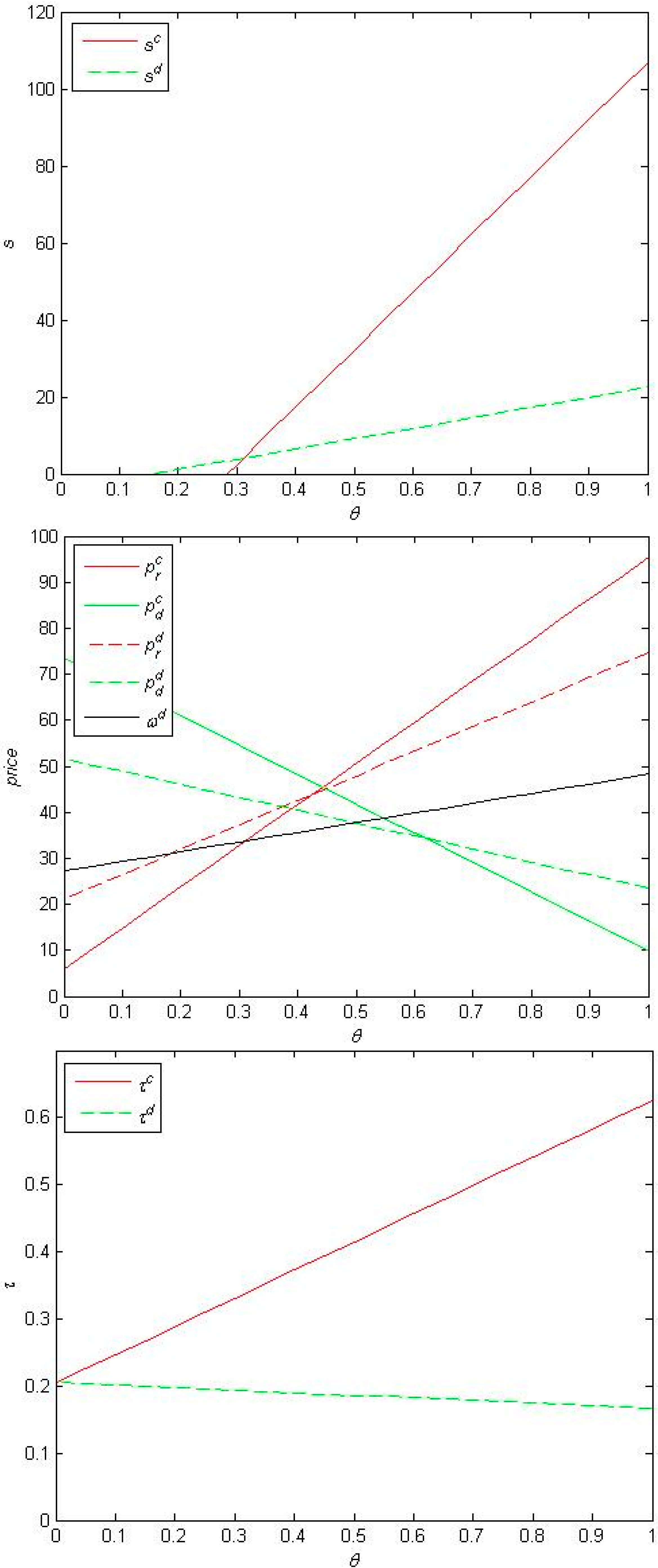
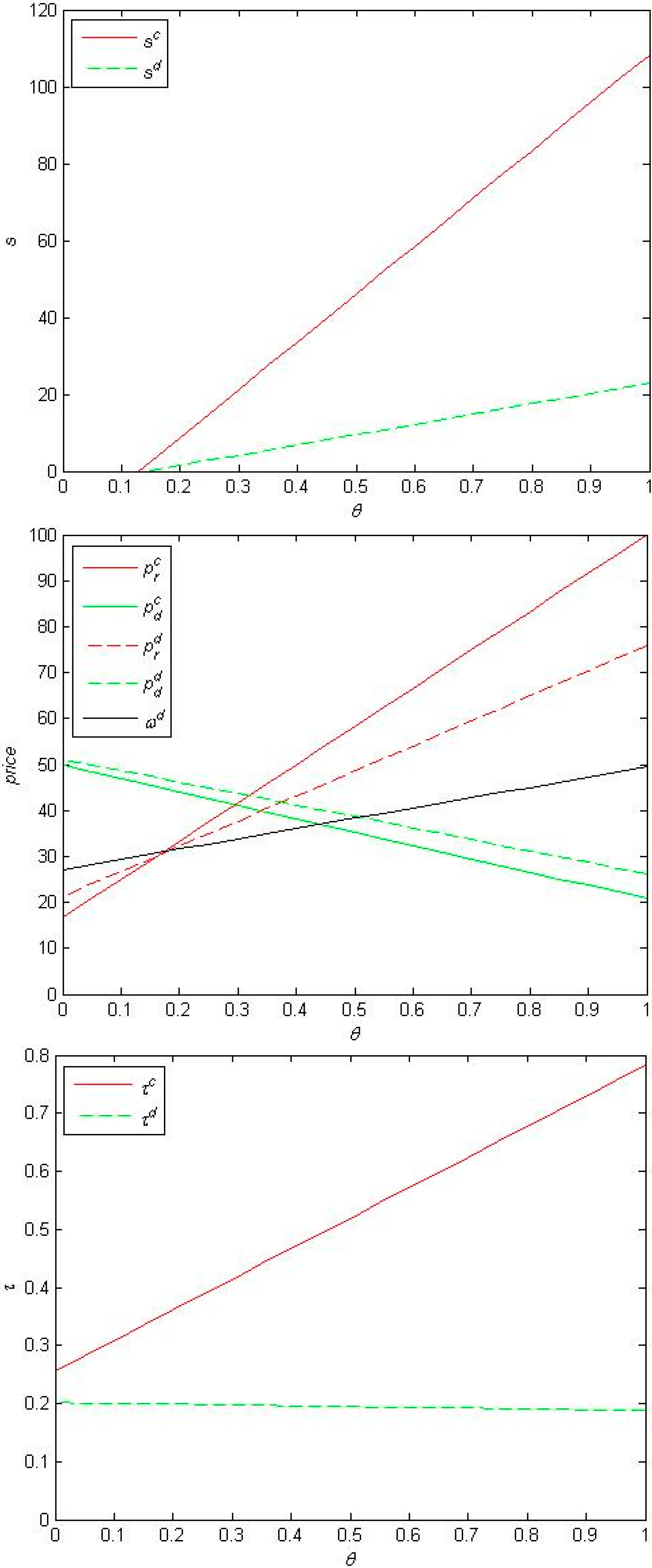
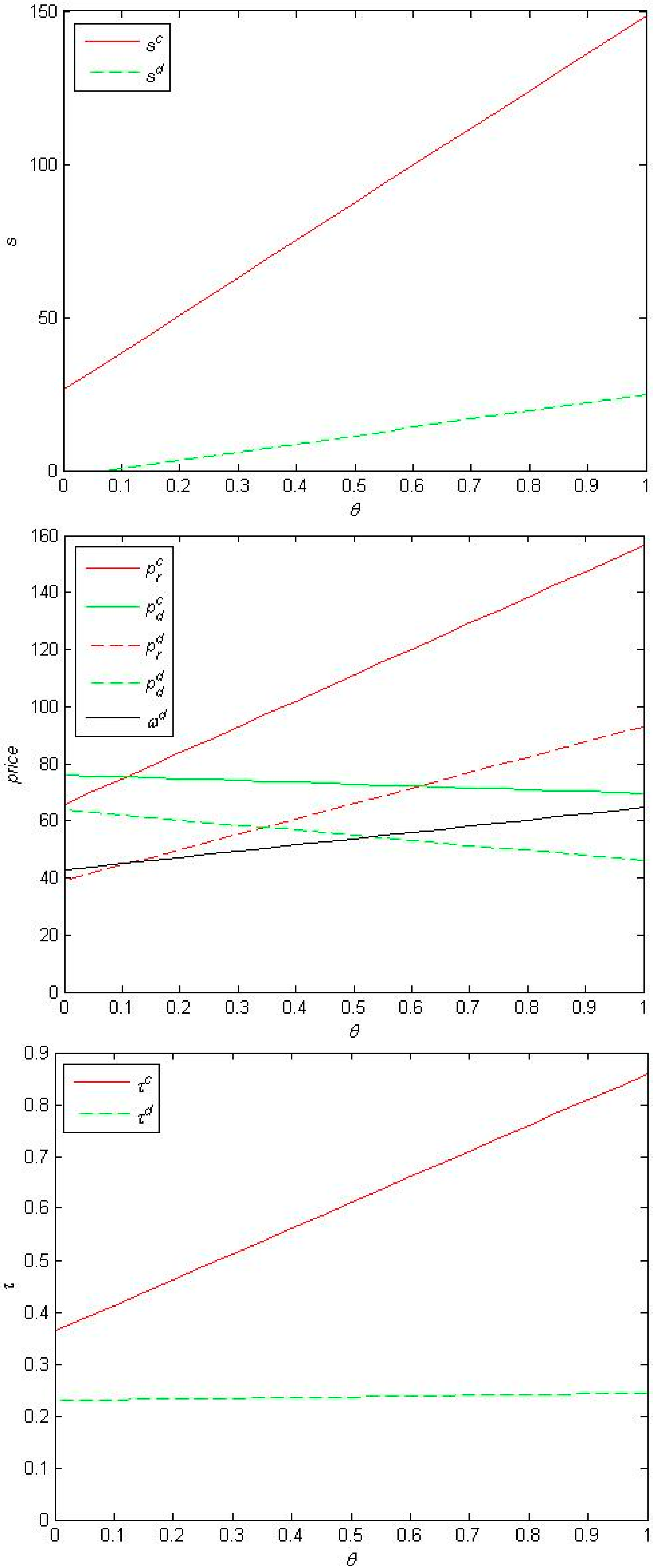
5. Numerical Examples

In this section, numerical examples are presented to verify our analytical results above and to analyze the differences between the centralized supply chain and the decentralized supply chain. The numerical examples are given in Table 1.
Table 1. Simulation settings in the numerical study.
ParameteracmcrCηβrβmb1b2bΔ
Value350205300045(2, 3)5(2, 3)1015

5.1. Centralized Case

In this subsection, we analyze the impacts of the ratio of relative increase of demand in the two channels and the degree of customer loyalty to the retail channel on the level of retail services, the retail price, the direct sale price and the return rate in the centralized dual-channel supply chain. From Figure 1, Figure 2 and Figure 3, for a fixed μ , the costs of retail services s c and the retail price p r c increase with the increase of the degree of customer loyalty to the retail channel θ . This means that the greater the base level of demand or the demand rate in the retail channel is, the higher the level of retail services and the retail price should be. However, the direct sale price p d c decreases with the increase of the degree of customer loyalty to the retail channel θ . We also obtain from Figure 1, Figure 2 and Figure 3 that the return rate τ c increases with the increase of the degree of customer loyalty to the retail channel θ .
Figure 1, Figure 2 and Figure 3 show that if the degree of customer loyalty to the retail channel is lower than a threshold, the cost of retail services will be very low. However, if the degree of customer loyalty to the retail channel is above a threshold, the direct sale price will be lower than the retail price. Therefore, we can conclude that when the degree of customer loyalty to the retail channel is relatively large, the retail price should be higher than the direct sale price.
Theoretically, the greater the demand in a single sale channel is, the larger the expected sale price should be. If the demand of products in one sale channel is relatively great, then the sale price in this sale channel should be set larger than that in the other sale channel. The above conclusions are also established in a dual-channel closed-loop supply chain.

5.2. Decentralized Case

In this subsection, we analyze the impacts of the ratio of the demand relative increase in the two channels and the degree of customer loyalty to the retail channel on the level of retail services, the retail price, the direct sale price, the whole sale price and the return rate in the decentralized dual-channel supply chain. From Figure 1, Figure 2 and Figure 3, for a fixed μ , the cost of retail services s d and the retail price p r d increase with the increase of the degree of customer loyalty to the retail channel θ , which means that the greater the base level of demand or demand rate in the retail channel is, the higher the level of retail services and the retail price should be. However, the direct sale price p d d decreases with the increase of the degree of customer loyalty to the retail channel θ . Figure 1, Figure 2 and Figure 3 also show that the degree of change of customer loyalty to the retail channel θ has little impact on the return rate τ d .
Figure 1, Figure 2 and Figure 3 also illustrate that when the degree of customer loyalty to the retail channel is relatively low, the direct sale price should be set higher than the retail price. However, if the degree of customer loyalty to the retail channel is above a threshold, the direct sale price should be set lower than the retail price. The degree of customer loyalty to the retail channel should be below a threshold in order to make the pricing strategy feasible.

5.3. Comparing the Two Settings

In this subsection, we compare the optimal retail services and the optimal pricing strategy in the two settings. From Figure 1, Figure 2 and Figure 3, when the ratio of the demand relative increase in the two channels is fixed, we obtain that the levels of retail services and the retail price increase with the increase of the degree of customer loyalty to the retail channel in both the centralized and decentralized systems. When the degree of customer loyalty to the retail channel is above a threshold, the levels of retail services and the retail price in the centralized system should be set higher than those in the decentralized system. We also find that the direct sale price decreases with the increase of the degree of customer loyalty to the retail channel in both the centralized and decentralized systems. When μ = 0 , the direct sale price in the decentralized system should be set higher than that in the centralized system; when μ < 0 , as the degree of customer loyalty to the retail channel is above a threshold, the direct sale price in the centralized system should be set lower than that in the decentralized system; when μ > 0 , as the degree of customer loyalty to the retail channel is above a threshold, the direct sale price in the decentralized system should be set lower than that in the centralized system. The changes in the degree of customer loyalty to the retail channel in the two settings have different impacts on the return rate.
Comparing the centralized and decentralized systems, we show that, in the decentralized setting, each player makes decisions based on the best profits for herself, but not for the whole system, so double marginalization exists in the decentralized dual-channel closed-loop supply chain. The results show that both the manufacturer and the retailer’s pricing decisions are strongly influenced by the retail services. We also find that the customer loyalty to the retail channel has impacts on their pricing decisions, but it has different impacts on the return rate.
Figure 1. Example 1 ( μ = 0.2 ).
Sustainability 07 02373 g001
Figure 2. Example 2 ( μ = 0 )
Sustainability 07 02373 g002
Figure 3. Example 3 ( μ = 0.2 ).
Sustainability 07 02373 g003

6. Conclusions

The retail services and pricing strategy are very important for the coordination of the dual sale channel. In this paper, we develop a dual-channel closed-loop supply chain model. We examine the impacts of the retail services and the degree of customer loyalty to the retail channel on the return rate and the pricing of players in a centralized and a decentralized dual-channel supply chain. We also make a comparison of the two settings. Then, we apply the two-stage optimization technique and Nash game theory to obtain the optimal retail services and the optimal pricing strategy.
We have some new findings that are different from earlier studies. Our results show that the retail services have a great impact on the pricing strategies of both manufacturers and retailers. At the same time, our numerical examples also show that retail services, retail price and direct sale price are all strongly influenced by the degree of customer loyalty to the retail channel and the ratio of the demand relative increase in the two channels with respect to the retail services, respectively. In a centralized supply chain, if the level of retail services is increased by the retailer, the retail price should be simultaneously increased. However, whether or not the manufacturer should simultaneously increase the direct sale price depends on the ratio of the demand relative increase in the two channels. When the ratio is negative, the direct sale price should decrease. When the ratio is zero, the direct sale price should stay constant. When the ratio is positive, the direct sale price should increase. However, in a decentralized dual-channel supply chain, if the level of retail services increases, the retail price should simultaneously increase, while the direct sale price should decrease. When the level of retail services is above a threshold, the wholesale price should simultaneously increase. When the level of retail services is below a threshold, whether or not the wholesale price should simultaneously increase depends on the ratio of the demand relative increase in the two channels. We also show that when the demand of products in one sale channel is relatively high, the sale price in this sale channel should be set greater than that in the other sale channel.
In future research, a number of assumptions in this paper can be relaxed. We assume that all of the players in the supply chain have access to the same information. Our results may not hold in practice because of the information asymmetry in the market. We also assume that all of the remanufactured products are of the same quality and price. However, many remanufactured products are sold at a lower price. For example, the Apple Store provides refurbished Apple products that are cheaper than the new ones. In reality, the demand for products in the market may not stay constant because of natural factors. Nonlinear sales response functions can also be investigated in future research.

Author Contributions

All authors contributed extensively to the work presented in this article. Zhen-Zheng Zhang wrote the paper with input from Zong-Jun Wang and Li-Wen Liu, discussing the results, implications and commenting on the manuscript at all stages.

Appendix

Proof of Proposition 1

Taking the second-order partial derivatives of c with respect to p r , p d , τ and s , we have the Hessian matrix: H c = ( c 2 s 2 c 2 s p r c 2 s p d c 2 s τ c 2 p r s c 2 p r 2 c 2 p r p d c 2 p r τ c 2 p d s c 2 p d p r c 2 p d 2 c 2 p d τ c 2 τ s c 2 τ p r c 2 τ p d c 2 τ 2 ) = ( η β r β m Δ ( β r β m ) β r 2 b 1 2 b 2 Δ ( b 1 b 2 ) β m 2 b 2 2 b 1 Δ ( b 1 b 2 ) Δ ( β r β m ) Δ ( b 1 b 2 ) Δ ( b 1 b 2 ) 2 C )
( 1 ) i D i , i = 1 , 2 , 3 , 4 .
When i = 1 , D 1 = ( η ) = η > 0 .
When i = 2 , D 2 = | η β r β r 2 b 1 | = 2 η b 1 β r 2 .
D 2 may be negative for large enough β r , so we cannot find that c is jointly concave in p r and s . We consider that H 1 is one of H c ’s submatrices, and we have:
H 1 = ( c 2 p r 2 c 2 p r p d c 2 p r τ c 2 p d p r c 2 p d 2 c 2 p d τ c 2 τ p r c 2 τ p d c 2 τ 2 ) = ( 2 b 1 2 b 2 Δ ( b 1 b 2 ) 2 b 2 2 b 1 Δ ( b 1 b 2 ) Δ ( b 1 b 2 ) Δ ( b 1 b 2 ) 2 C )
D 1 = ( 2 b 1 ) = 2 b 1 > 0
D 2 = | 2 b 1 2 b 2 2 b 2 2 b 1 | = 4 ( b 1 2 b 2 2 ) > 0
D 3 = | 2 b 1 2 b 2 Δ ( b 1 b 2 ) 2 b 2 2 b 1 Δ ( b 1 b 2 ) Δ ( b 1 b 2 ) Δ ( b 1 b 2 ) 2 C | = 8 C ( b 1 2 b 2 2 ) 4 Δ ( b 1 + b 2 ) ( b 1 b 2 ) 2 > 0
From the above results, we can conclude that c is strictly jointly concave in p r , p d and τ .
We differentiate c with respect to p r , p d and τ in Equation (8), respectively. Then, we have the following results:
c p r = 2 b 1 p r + 2 b 2 p d Δ τ ( b 1 b 2 ) + c m ( b 1 b 2 ) + β r s + θ a = 0
c p d = 2 b 2 p r 2 b 1 p d Δ τ ( b 1 b 2 ) + c m ( b 1 b 2 ) + β m s + ( 1 θ ) a = 0
c τ = Δ ( b 1 b 2 ) p r Δ ( b 1 b 2 ) p d 2 C τ + Δ s ( β r β m ) + Δ a = 0
From the above results, we have the optimal values of p r , p d and τ .
p r c * ( s ) = [ Δ 2 ( b 1 b 2 ) ( E F ) 4 C E + 2 Δ 2 ( β r β m ) ] s 2 c m [ 2 C + Δ 2 ( b 1 b 2 ) ] + Δ 2 ( b 1 b 2 ) ( A B ) 4 C A + 2 Δ 2 a 4 Δ 2 ( b 1 b 2 ) 8 C
p d c * ( s ) = [ Δ 2 ( b 1 b 2 ) ( F E ) 4 C F + 2 Δ 2 ( β r β m ) ] s 2 c m [ 2 C + Δ 2 ( b 1 b 2 ) ] + Δ 2 ( b 1 b 2 ) ( B A ) 4 C B + 2 Δ 2 a 4 Δ 2 ( b 1 b 2 ) 8 C
τ c * ( s ) = [ Δ ( b 1 b 2 ) ( E + F ) 2 Δ ( β r β m ) ] s + Δ ( b 1 b 2 ) [ 2 c m + ( A + B ) ] 2 Δ a 2 Δ 2 ( b 1 b 2 ) 4 C
Substituting p r c * ( s ) , p d c * ( s ) and τ c * ( s ) into Equation (8) and differentiating c with respect to s , we obtain the optimal s .
s c * = R Q
where:
R = 8 Δ 2 ( b 1 2 b 2 2 ) ( F E ) ( A B ) ( b 1 b 2 3 C ) + 32 C 2 ( b 2 A F b 1 A E + b 2 B E b 1 B F + β r A β m B ) + 16 a C Δ 2 ( b 1 b 2 ) ( E + F ) 8 C 2 Δ 2 ( b 1 b 2 ) ( A B ) + 4 Δ 4 ( b 1 b 2 ) 2 ( 3 A β m 3 B β r A β r B β m ) 16 C Δ 2 ( b 1 b 2 ) ( A β m B β r ) + 8 a Δ 4 ( b 1 b 2 ) ( β r β m ) 32 C 2 c m ( β r β m ) + 64 C c m Δ 2 ( b 1 b 2 ) ( β r β m ) 8 c m Δ 4 ( b 1 b 2 ) ( β r β m ) ( b 1 b 2 + 2 ) 8 Δ 4 ( β r β m ) [ ( b 1 b 2 ) ( A + B ) 2 a ] + [ 4 Δ 2 ( b 1 b 2 ) 8 C ] × [ ( 2 θ 3 ) a Δ 2 ( b 1 b 2 ) F ( 2 θ + 1 ) a Δ 2 ( b 1 b 2 ) E + 2 a Δ 2 ( β r β m ) + 4 a C ( θ E + F θ F ) ]
Q = 32 C 2 ( 2 β m F 2 β r E + E 2 + F 2 2 b 2 E F ) Δ 2 ( b 1 2 b 2 2 ) ( E F ) 2 ( 8 + 24 C ) + 16 C Δ 2 ( b 1 b 2 ) ( 3 β r E 3 β m F + β m E β r F ) 4 Δ 2 ( b 1 b 2 ) 2 ( β r + β m ) ( E F ) + 8 Δ 2 ( b 1 b 2 ) ( β r β m ) 2 8 C Δ 2 ( b 1 b 2 ) 2 ( E + F ) 2 4 Δ 4 ( b 1 b 2 ) 2 ( β m F β r E + 3 β m E β r F ) + 8 Δ 4 ( b 1 b 2 ) ( β r β m ) ( E + F 3 β r + 3 β m ) 16 Δ 4 ( β r β m ) 2 + η [ 4 Δ 2 ( b 1 b 2 ) 8 C ] 2

Proof of Proposition 2

Taking the first-order partial derivatives of p r c * ( s ) , p d c * ( s ) and τ c * ( s ) with respect to s , we have:
(1) p r c * ( s ) s = Δ 2 ( b 1 b 2 ) ( E F ) 4 C E + 2 Δ 2 ( β r β m ) 4 Δ 2 ( b 1 b 2 ) 8 C > 0
(2) p d c * ( s ) s = | Δ 2 ( b 1 b 2 ) ( F E ) 4 C F + 2 Δ 2 ( β r β m ) 4 Δ 2 ( b 1 b 2 ) 8 C |
When Δ 2 ( b 1 b 2 ) ( F E ) 4 C F + 2 Δ 2 ( β r β m ) 0 , E F 4 C F + 2 Δ 2 ( β r β m ) Δ 2 ( b 1 b 2 ) < 0 .
p r c * ( s ) s | p d c * ( s ) s | = Δ 2 ( b 1 b 2 ) ( E F ) 4 C E + 2 Δ 2 ( β r β m ) 4 Δ 2 ( b 1 b 2 ) 8 C ( Δ 2 ( b 1 b 2 ) ( F E ) 4 C F + 2 Δ 2 ( β r β m ) 4 Δ 2 ( b 1 b 2 ) 8 C > 0 ) = 8 C E + 4 Δ 2 ( E F ) 4 Δ 2 ( b 1 b 2 ) 8 C > 0
When Δ 2 ( b 1 b 2 ) ( F E ) 4 C F + 2 Δ 2 ( β r β m ) < 0 ,
p r c * ( s ) s | p d c * ( s ) s | = Δ 2 ( b 1 b 2 ) ( E F ) 4 C E + 2 Δ 2 ( β r β m ) 4 Δ 2 ( b 1 b 2 ) 8 C ( Δ 2 ( b 1 b 2 ) ( F E ) 4 C F + 2 Δ 2 ( β r β m ) 4 Δ 2 ( b 1 b 2 ) 8 C > 0 ) = 8 C E + 4 Δ 2 ( β r β m ) 4 Δ 2 ( b 1 b 2 ) 8 C > 0
(3) p d c * ( s ) s = | Δ 2 ( b 1 b 2 ) ( F E ) 4 C F + 2 Δ 2 ( β r β m ) 4 Δ 2 ( b 1 b 2 ) 8 C | = Δ 2 b 1 β r b 2 β m + 3 b 2 β r 4 b 1 β m b 1 + b 2 4 C β r b 2 β m b 1 b 1 2 b 2 2 4 Δ 2 ( b 1 b 2 ) 8 C
μ = ( β r β m β r ) ( b 1 b 2 b 1 ) = b 2 β r b 1 β m b 1 β r
When μ > 0 , p d c * ( s ) s > 0 ; when μ < 0 , p d c * ( s ) s < 0 ; when μ = 0 , p d c * ( s ) s = 0 .
(4) τ c * ( s ) s = Δ ( b 1 b 2 ) ( E + F ) 2 Δ ( β r β m ) 2 Δ 2 ( b 1 b 2 ) 4 C = Δ ( β r β m ) 2 Δ 2 ( b 1 b 2 ) 4 C > 0

Proof of Proposition 3

Taking the second-order partial derivatives of r with respect to p r , τ and s , we have the Hessian matrix:
H r = ( Π r 2 τ 2 Π r 2 τ p r Π r 2 τ s Π r 2 p r τ Π r 2 p r 2 Π r 2 p r s Π r 2 s τ Π r 2 s p r Π r 2 s 2 ) = ( 2 C b ( b 1 b 2 ) b ( β r β m ) b ( b 1 b 2 ) 2 b 1 β r b β m β r η )
Because 2 C > 0 , | 2 C b ( b 1 b 2 ) b ( b 1 b 2 ) 2 b 1 | = 4 b 1 C b 2 ( b 1 b 2 ) 2 > 0 . Obviously, the retailer’s profit Π r is strictly jointly concave in p r and τ . However, we still cannot confirm the sign of | 2 b 1 β r β r η | = β r 2 2 b 1 η , so Π r is not jointly concave in p r , τ and s . Similarly, we obtain that is Π m strictly jointly concave in w and p d , but not jointly concave in w , p d and s .
We differentiate Π r with respect to p r and τ in Equation (5), respectively. Then, we obtain the following results:
Π r p r = 2 b 1 p r b 2 p d + b ( b 1 b 2 ) τ b 1 w θ a β r s = 0
Π r τ = b ( b 1 b 2 ) p r + b ( b 1 b 2 ) p d + 2 C τ a b b ( β r β m ) s = 0
Substituting p r = w + m into Equation (6) and differentiating Π m with respect to w and p d , we obtain:
Π m w = b 1 p r 2 b 2 p d + ( Δ b ) ( b 1 b 2 ) τ + b 1 w θ a ( b 1 b 2 ) c m β r s = 0
Π m p d = b 2 p r 2 b 1 p d ( Δ b ) ( b 1 b 2 ) τ + b 2 w + ( 1 θ ) a + ( b 1 b 2 ) c m β m s = 0
From the above results, we have the optimal values of w , p r , p d and τ :
w d * = F s + 3 c m 7 B 2 3 b ( Δ b ) ( b 1 b 2 ) 4 C 2 b ( b 1 b 2 ) τ d * = b F G ( b 1 b 2 ) [ 3 b ( Δ b ) ( b 1 b 2 ) 4 C ] K 2 b ( b 1 b 2 ) G s + 3 b ( b 1 b 2 ) [ 3 b ( Δ b ) ( b 1 b 2 ) 4 C ] D 2 b ( b 1 b 2 ) G c m 7 b B G ( b 1 b 2 ) [ 3 b ( Δ b ) ( b 1 b 2 ) 4 C ] H 2 b ( b 1 b 2 ) G
p r d * = [ 2 ( β r β m ) F ( b 1 b 2 ) ] b s b ( b 1 b 2 ) c m + 2 a b b B ( b 1 b 2 ) + [ b ( Δ b ) ( b 1 b 2 ) 4 C ] τ d * 2 b ( b 1 b 2 ) = [ 2 ( β r β m ) F ( b 1 b 2 ) ] b G + [ b ( Δ b ) ( b 1 b 2 ) 4 C ] K 2 b ( b 1 b 2 ) G s b ( b 1 b 2 ) [ b ( Δ b ) ( b 1 b 2 ) 4 C ] D 2 b ( b 1 b 2 ) G c m + 2 a b b B ( b 1 b 2 ) + [ b ( Δ b ) ( b 1 b 2 ) 4 C ] H 2 b ( b 1 b 2 ) G
p d d * = F s + c m + B ( Δ b ) τ d * 2 = [ F 2 ( Δ b ) K 2 G ] s + [ 1 2 ( Δ b ) D 2 G ] c m + B 2 ( Δ b ) H 2 G
τ d * = K s + D c m + H G
where:
K = 3 ( b 1 β m 2 b 1 β r b 2 β r ) b
D = ( 5 b 1 + b 2 ) ( b 1 b 2 ) b
H = 3 a b ( θ b 1 θ b 2 b 1 )
G = 3 a b ( Δ b ) ( b 1 2 b 2 2 ) + 2 Δ b ( b 1 b 2 ) 2 12 b 1 C
Substituting w d * , p r d * , p d d * and τ d * into Equation (5) and differentiating Π r with respect to s , we obtain:
r s = { [ F 2 ( Δ b ) K 2 G ] b 2 + β r b ( b 1 b 2 ) K G + b b 1 F G ( b 1 b 2 ) b 1 [ 3 b ( Δ b ) ( b 1 b 2 ) 4 C ] K 2 b ( b 1 b 2 ) G } × { 2 ( β r β m ) F ( b 1 b 2 ) b G [ b ( Δ b ) ( b 1 b 2 ) 4 C ] K 2 b ( b 1 b 2 ) G s b ( b 1 b 2 ) [ b ( Δ b ) ( b 1 b 2 ) 4 C ] D 2 b ( b 1 b 2 ) G c m + 2 a b b B ( b 1 b 2 ) + [ b ( Δ b ) ( b 1 b 2 ) 4 C ] H 2 b ( b 1 b 2 ) G } + { 2 ( β r β m ) F ( b 1 b 2 ) b b 2 G + [ b ( Δ b ) ( b 1 b 2 ) 4 C ] b 2 K 2 b ( b 1 b 2 ) G b b 2 F G ( b 1 b 2 ) [ 3 b ( Δ b ) ( b 1 b 2 ) 4 C ] b 2 K 2 b ( b 1 b 2 ) G b ( b 1 b 2 ) K G } × { [ F 2 ( Δ b ) K 2 G ] s + [ 1 2 ( Δ b ) D 2 G ] c m + B 2 ( Δ b ) H 2 G } + { [ 2 ( β r β m ) F ( b 1 b 2 ) ] b b 1 G + [ b ( Δ b ) ( b 1 b 2 ) 4 C ] b 1 K 2 b ( b 1 b 2 ) G [ b 2 F 2 ( Δ B ) b 2 K 2 G ] } × { b F G ( b 1 b 2 ) [ 3 b ( Δ b ) ( b 1 b 2 ) 4 C ] K 2 b ( b 1 b 2 ) G s + 3 b ( b 1 b 2 ) G [ 3 b ( Δ b ) ( b 1 b 2 ) 4 C ] D 2 b ( b 1 b 2 ) G c m 7 b B G ( b 1 b 2 ) + [ 3 b ( Δ b ) ( b 1 b 2 ) 4 C ] H 2 b ( b 1 b 2 ) G } + { b ( β r β m ) b ( b 1 b 2 ) 2 ( β r β m ) F ( b 1 b 2 ) b G + [ b ( Δ b ) ( b 1 b 2 ) 4 C ] K 2 b ( b 1 b 2 ) G b ( b 1 b 2 ) [ F 2 ( Δ b ) K 2 G ] 2 C K G } × { K s + D c m + H G } + { 2 ( β r β m ) F ( b 1 b 2 ) b β r G + [ b ( Δ b ) ( b 1 b 2 ) 4 C ] β r K 2 b ( b 1 b 2 ) G + b ( β r β m ) K G η } s + ( θ a 2 b 1 ) [ 2 ( β r β m ) F ( b 1 b 2 ) ] b G + [ b ( Δ b ) ( b 1 b 2 ) 4 C ] K 2 b ( b 1 b 2 ) G + a b K G θ a b F G ( b 1 b 2 ) [ 3 b ( Δ b ) ( b 1 b 2 ) 4 C ] K 2 b ( b 1 b 2 ) G = 0
We can get the optimal
s :
s d * = N M
where:
M = { 2 β r b ( b 1 b 2 ) G b b 2 ( Δ b ) ( b 1 b 2 ) K + b b 1 F G ( b 1 2 b 2 2 ) b 1 [ 3 b ( Δ b ) ( b 1 b 2 ) 4 C ] K 2 b 2 ( b 1 b 2 ) 2 K } { [ 2 ( β r β m ) F ( b 1 b 2 ) ] b G + [ b ( Δ b ) ( b 1 b 2 ) 4 C ] K } + { [ 2 ( β r β m ) F ( b 1 b 2 ) ] b b 2 G + [ b ( Δ b ) ( b 1 b 2 ) 4 C ] b 2 K 2 b 2 ( b 1 b 2 ) 2 K b b 2 F G ( b 1 b 2 ) + [ 3 b ( Δ b ) ( b 1 b 2 ) 4 C ] b 2 K } { F b ( b 1 b 2 ) G b ( b 1 b 2 ) ( Δ b ) K } + { [ 2 ( β r β m ) F ( b 1 b 2 ) ] b b 1 G + [ b ( Δ b ) ( b 1 b 2 ) 4 C ] b 1 K b 2 b ( b 1 b 2 ) G F + ( Δ b ) b ( b 1 b 2 ) b 2 K } { b F G ( b 1 b 2 ) [ 3 b ( Δ b ) ( b 1 b 2 ) 4 C ] K } + 2 b ( b 1 b 2 ) K { 2 b 2 ( b 1 b 2 ) ( β r β m ) G [ 2 ( β r β m ) F ( b 1 b 2 ) ] b 2 ( b 1 b 2 ) G 4 C b ( b 1 b 2 ) K [ b ( Δ b ) ( b 1 b 2 ) 4 C ] b ( b 1 b 2 ) K + b 2 ( b 1 b 2 ) 2 ( Δ b ) K b 2 ( b 1 b 2 ) 2 G F } + [ 2 ( β r β m ) F ( b 1 b 2 ) ] b β r G + [ b ( Δ b ) ( b 1 b 2 ) 4 C ] β r K + 2 b 2 ( b 1 b 2 ) ( β r β m ) K 2 η b ( b 1 b 2 ) G
N = { b 1 [ 3 b ( Δ b ) ( b 1 b 2 ) 4 C ] K 2 β r b ( b 1 b 2 ) G + b b 2 ( Δ b ) ( b 1 b 2 ) K + 2 b 2 ( b 1 b 2 ) 2 K b b 1 F G ( b 1 2 b 2 2 ) } { [ b ( Δ b ) ( b 1 b 2 ) 4 C ] c m D b c m ( b 1 b 2 ) + 2 a b b B ( b 1 b 2 ) + [ b ( Δ b ) ( b 1 b 2 ) 4 C ] H } + { 2 b 2 ( b 1 b 2 ) 2 K b b 2 F G ( b 1 b 2 ) [ 2 ( β r β m ) F ( b 1 b 2 ) ] b b 2 G [ b ( Δ b ) ( b 1 b 2 ) 4 C ] b 2 K [ 3 b ( Δ b ) ( b 1 b 2 ) 4 C ] b 2 K } [ b ( b 1 b 2 ) c m G b c m ( Δ b ) ( b 1 b 2 ) D + b ( b 1 b 2 ) G B b ( b 1 b 2 ) ( Δ b ) H ] + { [ 2 ( β r β m ) F ( b 1 b 2 ) ] b b 1 G [ b ( Δ b ) ( b 1 b 2 ) 4 C ] b 1 K + b 2 b ( b 1 b 2 ) G F + ( Δ b ) b ( b 1 b 2 ) b 2 K } { 3 b c m ( b 1 b 2 ) G [ 3 b ( Δ b ) ( b 1 b 2 ) 4 C ] c m D 7 b B G ( b 1 b 2 ) [ 3 b ( Δ b ) ( b 1 b 2 ) 4 C ] H } + { 2 b 2 ( b 1 b 2 ) ( β r β m ) G 4 c b ( b 1 b 2 ) K + [ 2 ( β r β m ) F ( b 1 b 2 ) ] b 2 ( b 1 b 2 ) G + [ b ( Δ b ) ( b 1 b 2 ) 4 C ] b ( b 1 b 2 ) K b 2 ( b 1 b 2 ) 2 ( Δ B ) K b 2 ( b 1 b 2 ) 2 G F } [ 2 b ( b 1 b 2 ) D c m + 2 b ( b 1 b 2 ) H ] [ 2 ( β r β m ) F ( b 1 b 2 ) ] b ( θ a 2 b 1 ) G [ b ( Δ b ) ( b 1 b 2 ) 4 C ] ( θ a 2 b 1 ) K 2 a b 2 ( b 1 b 2 ) K + θ a b F G ( b 1 b 2 ) θ a [ 3 b ( Δ b ) ( b 1 b 2 ) 4 c ] K

Proof of Proposition 4

Taking the first-order partial derivatives of w d * ( s ) , p r d ( s ) , p d d ( s ) and τ d ( s ) with respect to s , we have:
(1) w d * s = F 2 [ 3 b ( Δ b ) ( b 1 b 2 ) 4 C ] K 2 b ( b 1 b 2 ) G > 0
(2) p r d s = [ 2 ( β r β m ) F ( b 1 b 2 ) ] b G + [ b ( Δ b ) ( b 1 b 2 ) 4 C ] K 2 b ( b 1 b 2 ) G > 0
(3) | p d d s | = | F 2 ( Δ b ) K 2 G | p r d s w d * s = [ 2 ( β r β m ) F ( b 1 b 2 ) ] b G + [ b ( Δ b ) ( b 1 b 2 ) 8 C ] K 2 b ( b 1 b 2 ) G F 2 > 0 w d * s | p d d s | = F 2 [ 3 b ( Δ b ) ( b 1 b 2 ) 4 C ] K | b ( b 1 b 2 ) F G b ( b 1 b 2 ) ( Δ b ) K | 2 b ( b 1 b 2 ) G > 0
(4) τ d s = K G = 3 ( b 1 β m 2 b 1 β r b 2 β r ) b 3 b ( Δ b ) ( b 1 2 b 2 2 ) + 2 Δ b ( b 1 b 2 ) 2 12 b 1 C < 0

Conflict of Interests

The authors declare no conflict of interest.

References

  1. Chen, R.J.C. From sustainability to customer loyalty: A case of full service hotels’ guests. J. Retail. Consum. Serv. 2014, 22, 261–265. [Google Scholar] [CrossRef]
  2. Devika, K.; Jafarian, A.; Nourbakhsh, V. Designing a sustainable closed-loop supply chain network based on triple bottom line approach: A comparison of metaheuristics hybridization techniques. Eur. J. Oper. Res. 2014, 235, 594–615. [Google Scholar] [CrossRef]
  3. Sasikumar, P. Issues in reverse supply chains, part II: Reverse distribution issues—An overview. Int. J. Sustain. Eng. 2008, 1, 234–249. [Google Scholar] [CrossRef]
  4. Tedeschi, B. Compressed data; big companies go slowly in devising net strategy. New York Times 2000. [Google Scholar]
  5. Chiang, W.Y.K.; Chhajed, D.; Hess, J.D. Direct-marketing, indirect profits: A strategic analysis of dual-channel supply-chain design. Manag. Sci. 2003, 49, 1–20. [Google Scholar] [CrossRef]
  6. Tsay, A.A.; Agrawal, N. Channel conflict and coordination in the E-commerce age. Prod. Oper. Manag. 2004, 13, 93–110. [Google Scholar] [CrossRef]
  7. Seifert, R.W.; Thonemann, U.W.; Hausman, W.H. Optimal procurement strategies for online spot markets. Eur. J. Oper. Res. 2004, 152, 781–799. [Google Scholar] [CrossRef]
  8. Cai, G.S. Channel Selection and Coordination in Dual-Channel Supply Chains. J. Retail. 2010, 86, 22–36. [Google Scholar] [CrossRef]
  9. Chen, K.Y.; Kaya, M.; Ozer, O. Dual Sales Channel Management with Service Competition. Manuf. Serv. Oper. Manag. 2008, 10, 654–675. [Google Scholar]
  10. Yan, R.; Pei, Z. Retail services and firm profit in a dual-channel market. J. Retail. Consum. Serv. 2009, 16, 306–314. [Google Scholar] [CrossRef]
  11. Dumrongsiri, A.; Fan, M.; Jain, A.; Moinzadeh, K. A supply chain model with direct and retail channels. Eur. J. Oper. Res. 2008, 187, 691–718. [Google Scholar] [CrossRef]
  12. Hu, W.; Li, Y.J. Retail service for mixed retail and E-tail channels. Ann. Oper. Res. 2012, 192, 151–171. [Google Scholar] [CrossRef]
  13. Yao, D.Q.; Liu, J.J. Competitive pricing of mixed retail and e-tail distribution channels. Omega-Int. J. Manag. Sci. 2005, 33, 235–247. [Google Scholar] [CrossRef]
  14. Hall, J.; Porteus, E. Customer service competition in capacitated systems. Manuf. Serv. Oper. Manag. 2000, 2, 144–165. [Google Scholar]
  15. Bernstein, F.; Federgruen, A. A general equilibrium model for industries with price and service competition. Oper. Res. 2004, 52, 868–886. [Google Scholar] [CrossRef]
  16. Boyaci, T.; Gallego, G. Supply chain coordination in a market with customer service competition. Prod. Oper. Manag. 2004, 13, 3–22. [Google Scholar] [CrossRef]
  17. Cai, G.; Zhang, Z.G.; Zhang, M. Game theoretical perspectives on dual-channel supply chain competition with price discounts and pricing schemes. Int. J. Prod. Econ. 2009, 117, 80–96. [Google Scholar] [CrossRef]
  18. Kurata, H.; Yao, D.Q.; Liu, J.J. Pricing policies under direct vs. indirect channel competition and national vs. store brand competition. Eur. J. Oper. Res. 2007, 180, 262–281. [Google Scholar] [CrossRef]
  19. Geng, Q.; Mallik, S. Inventory competition and allocation in a multi-channel distribution system. Eur. J. Oper. Res. 2007, 182, 704–729. [Google Scholar] [CrossRef]
  20. Chiang, W.Y.K. Product availability in competitive and cooperative dual-channel distribution with stock-out based substitution. Eur. J. Oper. Res. 2010, 200, 111–126. [Google Scholar] [CrossRef]
  21. Boyaci, T. Competitive stocking and coordination in a multiple-channel distribution system. IIE Trans. 2005, 37, 407–427. [Google Scholar] [CrossRef]
  22. Majumder, P.; Groenevelt, H. Competition in remanufacturing. Prod. Oper. Manag. 2001, 10, 125–141. [Google Scholar] [CrossRef]
  23. Teunter, R.H.; Flapper, S.D.P. Optimal core acquisition and remanufacturing policies under uncertain core quality fractions. Eur. J. Oper. Res. 2011, 210, 241–248. [Google Scholar] [CrossRef]
  24. Savaskan, R.C.; Bhattacharya, S.; van Wassenhove, L.N. Closed-loop supply chain models with product remanufacturing. Manag. Sci. 2004, 50, 239–252. [Google Scholar] [CrossRef]
  25. Gu, Q.L.; Ji, J.H.; Gao, T.G. Pricing management for a closed-loop supply chain. J. Revenue Pricing Manag. 2008, 7, 45–60. [Google Scholar] [CrossRef]
  26. Savaskan, R.C.; van Wassenhove, L.N. Reverse channel design: The case of competing retailers. Manag. Sci. 2006, 52, 1–14. [Google Scholar] [CrossRef]
  27. Qiang, Q.; Ke, K.; Anderson, T.; Dung, J. The closed-loop supply chain network with competition, distribution channel investment, and uncertainties. Omega-Int. J. Manag. Sci. 2013, 41, 186–194. [Google Scholar] [CrossRef]
  28. Ozkir, V.; Basligil, H. Modelling product-recovery processes in closed-loop supply-chain network design. Int. J. Prod. Res. 2012, 50, 2218–2233. [Google Scholar] [CrossRef]
  29. Neto, J.Q.F.; Walther, G.; Bloemhof, J.; van Nunen, J.; Spengler, T. From closed-loop to sustainable supply chains: The WEEE case. Int. J. Prod. Res. 2010, 48, 4463–4481. [Google Scholar] [CrossRef]
  30. Georgiadis, P.; Athanasiou, E. Flexible long-term capacity planning in closed-loop supply chains with remanufacturing. Eur. J. Oper. Res. 2013, 225, 44–58. [Google Scholar] [CrossRef]
  31. Chen, J.; Bell, P.C. Implementing market segmentation using full-refund and no-refund customer returns policies in a dual-channel supply chain structure. Int. J. Prod. Econ. 2012, 136, 56–66. [Google Scholar] [CrossRef]
  32. Hong, X.P.; Wang, Z.J.; Wang, D.Z.; Zhang, H.G. Decision models of closed-loop supply chain with remanufacturing under hybrid dual-channel collection. Int. J. Adv. Manuf. Technol. 2013, 68, 1851–1865. [Google Scholar] [CrossRef]
  33. Hua, G.W.; Wang, S.Y.; Cheng, T.C.E. Price and lead time decisions in dual-channel supply chains. Eur. J. Oper. Res. 2010, 205, 113–126. [Google Scholar] [CrossRef]
  34. Dan, B.; Xu, G.Y.; Liu, C. Pricing policies in a dual-channel supply chain with retail services. Int. J. Prod. Econ. 2012, 139, 312–320. [Google Scholar] [CrossRef]
  35. Corbett, C.J.; de Groote, X. A supplier’s optimal quantity discount policy under asymmetric information. Manag. Sci. 2000, 46, 444–450. [Google Scholar] [CrossRef]

