An Application of the Short-Term Forecasting with Limited Data in the Healthcare Traveling Industry

Abstract

In real practice, forecasting under the limited data has attracted more attention in business activities, especially in the healthcare traveling industry in its current stage. However, there are only a few research studies focusing on this issue. Thus, the purposes of this paper were to determine the forecasted performance of several current forecasting methods as well as to examine their applications. Taking advantage of the small data requirement for model construction, three models including the exponential smoothing model, the Grey model GM(1,1), and the modified Lotka-Volterra model (L.V.), were used to conduct forecasting analyses based on the data of foreign patients from 2001 to 2013 in six destinations. The results indicated that the L.V. model had higher prediction power than the other two models, and it obtained the best forecasting performance with an 89.7% precision rate. In conclusion, the L.V. model is the best model for estimating the market size of the healthcare traveling industry, followed by the GM(1,1) model. The contribution of this study is to offer a useful statistical tool for short-term planning, which can be applied to the healthcare traveling industry in particular, and for other business forecasting under the conditions of limited data in general.

1. Introduction

Healthcare traveling, also known as the medical tourism industry, is a type of service industry which is a combination of healthcare or medical treatments and tourism services. The development of the healthcare traveling industry is a product of the rise of private healthcare demand, the globalization of healthcare services, the rapid development of the Internet, and the increasing providers of low-cost traveling abroad. Therefore, sustainable development of the healthcare traveling industry has an important role for promoting and enhancing the level of social-economic performance of nations. Crucial factors that cause most foreign patients to look for access to therapeutic procedures across borders include the shortage of medical availability, lengthy waiting lists, or the affordability of treatments [1,2]. In addition, from the viewpoint of patients, seeking the advanced medical surgeries in foreign nations is also a main factor for healthcare traveling. As a result, there is a phenomenon of patient movement from developed countries to less developed countries, so that they can receive a high medical standard of healthcare, treatment, or beauty services through traveling [3]. In fact, the demand for out-of-pocket healthcare and medical services abroad is increasing around the world. According to [4], in 2019, the global medical tourism market will be have a market worth of 32.5 billion USD. The market size of this industry has been quickly expanding, which has created lucrative businesses on healthcare services, tourism services, and related businesses. In recognition of the potential contributions of healthcare traveling on economic development, several countries have been defined healthcare traveling as a core industry at the national level. Utilizing the advantages of medical technologies and tourism resources, governments have been investing more money in healthcare and medical infrastructure, as well as proposing promotion campaigns aimed at developing this industry. Some successful cases include Hungary, Belgium, Turkey, Poland, Mexico, Brazil, India, Thailand, Singapore, Malaysia, Korea, Taiwan, etc.

With the full effort and encouragement of the government, as well as the success of taking advantage of the competitive prices of medical services, advanced technologies in medical specialties, flexible treatment processes, and effective business strategies of the service providers, some countries in Asia including Thailand, Korea, Singapore, India, Malaysia, Thailand, and Taiwan have created their own accreditation system for exporting medical services to the global market. Although these countries joined the global market for healthcare traveling quite late compared to numerous destinations in Europe such as Hungary, Belgium, Spain, Czech Republic, Poland, etc., the performance of the countries in Asia has received close attention. Actually, the foreign patients from developed countries toward these countries for receiving healthcare and medical services, especially for healthcare screening, medical treatments, beauty or sex changes procedures, etc are increasing. Furthermore, along with the rise of China’s economy, the GDP and private income of people have been improving, and the medical tourism demand from Chinese patients has also made the Asian medical tourism market more lively in recent years. Within a decade, this area has become a popular destination of healthcare traveling with world class standards. This area continues to attract a large number of foreign medical tourists from around the world, compared to other areas. Among the Asian countries, Thailand and Singapore are far ahead with approximately 90% of the foreign patients in this area [5]. Statistical data of the number of medical tourists in six major destinations in Asia are presented in

Table 1. Number of medical tourists in the healthcare industry (persons).

Years	Destinations
	Malaysia	Singapore	Thailand	Korea	Taiwan	India
2001	75,210
2002	84,585
2003	102,946		730,000
2004	147,189	320,000	1,103,905
2005	232,161	370,000	1,249,984			153,000
2006	296,689	410,000	1,450,000			230,000
2007	341,228	571,000	1,540,000			450,000
2008	374,063	646,000	1,300,000	27,480	21,974	530,000
2009	336,225	665,000	1,500,000	60,201	83,496	609,000
2010	392,956	725,000	1,980,000	81,789	110,664	731,000
2011	583,296	359,590	2,240,000	122,297	109,133
2012	671,227	850,000	2,400,000	159,464	173,081
2013	770,134		2,530,000	211,218	100,083

Sources: [6,7,8,9,10,11,12,13].

.

As mentioned above, the growth of healthcare traveling in Asia has been booming, and it has been assessed as a lucrative industry. Moreover, promoting sustainable development of this industry will help maintain three major sections of the host countries, including the environment, the economy, and the local community [14]. Particularly, the development of the healthcare traveling industry has not only positively impacted the quality of the local medical systems directly but has also played a crucial role in promoting related businesses, especially for the tourism industry. Therefore, it is necessary to have a reliable tool to estimate the market size of this industry in order to understand the changes in future demands. A suitable forecasting approach can help policymakers and stakeholders propose the correct strategies for their business activities. However, obtaining full data is a big problem for the healthcare traveling industry as discussed previously. Therefore, the idea of this study was to find numerous high predictive models which can apply to predict the demand of the healthcare travelling industry under the condition of small data points for model construction.

Regarding the forecasting of tourism demand, research in [15] addressed that forecasting accuracy is especially important and acute for the tourism industry because of the perishability of tourism. Based on the output of forecasting models, information can be utilized by policymakers to make different policy decisions under particular circumstances as “tourism flows have consequences for a wide range of different policy-making situation” [16]. Most of the current studies focused on the application of quantitative forecasting techniques with time series, econometric models, and some new techniques such as artificial intelligence (AI), artificial neural networks (ANNs), genetic algorithms (GAs), etc. [17] in various destinations. However, the performance of the forecast model relies on data frequencies used in the model estimation, destination-origin country/region pairs under consideration, and the length of the forecasting horizons concerned [18].

Asia’s healthcare traveling industry is still in its early stages, and thus gaining reliable data on the volume of consumption of health services aboard is challenging. In addition, the limited data from this industry cannot support the traditional approaches for long-term forecasts. Therefore, short-term forecast techniques using limited historical data can be considered. Previous literature [19] applied the GM(1,1) alpha model to forecast the demand for healthcare tourism in some Asian countries. However, this model did not perform well (the mean absolute percent error or MAPE is 29.1%) with India’s healthcare service provider. Aside from the GM(1,1) model, the time series autoregressive integrated moving average (ARIMA )model was also implemented to predict the demand for medical tourism in India [20]. The scope of this study only focused on a number of medical tourist arrivals from different countries traveling to India to receive healthcare services. Despite the fact that existing studies on medical tourism indicate that the businesses relative to the healthcare travelling are the large market for exploration, the estimation for this demand is regarded at a particular destination. Thus, the application of prediction methods in this industry still need to be developed.

As mentions above, it is necessary to have a high accuracy model to forecast the demand of the healthcare traveling industry. An effective tool for predicting play a crucial role in the process of decision making, which helps the policy makers, healthcare service providers, tourism industry leaders, as well as related service managers clearly recognize the changing in the future. To address the forecasting process using limited past information, as well as to determine the application scope of the proposed models in real practice, three models including the exponential smoothing model of time series forecast, the grey model, and the Lotka-Votterra (L.V.) model [21], were applied with the data of tourist arrivals of the healthcare traveling industry in six major medical destinations in Asia, as shown in Table 1. Finally, the forecasting power of the three forecasting models was also computed based on evaluating the precision rate of the forecasting models.

Following this section, in the next section we present the theoretical foundations related to the short-term forecasting and literature reviews of the three proposed forecasting models. The methodology is described in Section 3. The empirical results and discussion are presented in Section 4. Section 5 outlines the conclusions of this paper.

2. Theoretical Foundation

In this section, we present the discussions on short-term forecasting and the literature reviews of some forecast models with small data sets.

Forecasting is a crucial procedure in business strategic planning. Organization managers use forecast information for most of their business decisions. Thus, a trustworthy forecast cannot only help companies clearly recognize the future opportunities, but it can also reduce potential risks as well as fully utilize company resources. According to different business planning techniques and characteristics of each industry, managers intend to employ different time horizon based forecast techniques to estimate future demand. Generally speaking, the time horizon forecast will be segmented into three types including short-term, medium-term, and long-term forecasts. However, along with the rapid development of the internet and economic exchanges, business environments around the world are also rapidly changing, and therefore forecasting accuracy has been impacted by more uncertainty factors. As a result, many strategists have adopted short-term forecasting methods in order to respond to the change of business environments in real-time. Short-term forecasts have been popularly utilized in demand estimation, inventory control, finance, etc. A good short-term forecast will not only expand enterprise’s profits based on reduced inventory level and enhanced customer service levels, but it will also increase the prediction credibility of the organization [22].

Worthwhile information for business decisions is achieved by the output of a reliable forecast model, and thus choosing the right model for forecasting is crucial for the entire forecasting process. The right model is utilized as an effective tool to help forecasters realize the changing future trends. There are a few criteria used to help select a suitable forecast model. However, the data that is available and the data characteristics are the crucial criteria that impact the model selection. Some guides to determine suitable forecasting models based on the data requirements for several common forecasting models are summarized in

Table 2. Historical data requirement for several forecast models.

Forecast Models	Data Requirement	Time Horizon for Forecasting
Moving average	2 to 30	Short
Simple exponential smoothing	5 to 10	Short
Trend models	10 to 20	Short, medium
Casual regression models	10 observations per independent variable	Short, medium, or long
Box–Jenkins	50	Long
Neural network	Large number	Short
Grey models	4	Short, medium, or long

Source: [23,24].

. According to that, when the data sample size is small, only a few models can be used. Notice that, in this study “short-term forecasting” means forecasting for one or two following periods, and the forecasting process has been assumed slow incremental change. Therefore, between one or two periods and the next one, the time series can be rendered approximately stationary. Thus, we can predict that its statistical properties will be the same in the future as they have been in the past.

Even though forecasts are a vital part of an organization’s activities, its process still relies on historical information. However, full data is not always easy to obtain in real situations, such as the estimation of the demand of a new product, new services businesses, etc. Therefore, accurate forecasts with limited historical data have garnered the attention of researchers and company managers [23].

2.1. The Time Series Forecasting Using Exponential Smoothing

Presently, the traditional statistical approach offers some time series forecasting models which are commonly used in business forecasting. Time series forecasting models mainly predict the future change based on understanding the past data, that may contain one or more component: trend, seasonal, cyclical, autocorrelation, and random. Several popular time series models are ARIMA models, structural models, the generalized autoregressive conditional heteroskedasticity (GARCH) models, neural networks, etc. However, most of the models require the use of large amounts of historical data in order to ensure the stationary of the forecast model.

Exponential smoothing forecasting is one model of time series which is popularly applied in business forecasting. According to the information in Table 2, this model takes advantage of the small data requirement, simple computation, and emphasizes the most up-to-date information compared to the rest of the models. As a result, the exponential smoothing has been determined to be an extremely valuable tool for short-term planning and inventory control with high forecast accuracy [25,26,27,28].

2.2. The Grey Forecasting

Besides the traditional forecasting approach mentioned above, the grey prediction is also used as a popular forecasting tool under the conditions of limited observations and uncertainty circumstances. As part of the grey system theory which was developed in 1989 by Deng [29], grey prediction models mainly focus on sequence prediction, disaster prediction, seasonal prediction, topology prediction, and composite prediction. Several common grey prediction models include the GM(1,1), the grey Verhulst, the DGM(1,1) [29], etc. Compared with traditional statistical forecast models, the historical data requirement for model construction of grey predictions can be minimized to at least four data points, the mathematical background for modeling is quite simple, and the forecast performance has high accuracy. For these reasons, grey prediction models have been widely utilized in the different fields of business forecasting, in both previous and current studies [23,30,31,32,33]. Therefore, grey predictions have become a favorite short-term forecasting technique for understanding the statements with limited past information or difficult to obtain data in the recent three decades. Until now, the application, exploration, and improvement of grey forecasts has been proposed in scholarly research and real applications.

2.3. The Lotka-Vottera System

The original Lotka-Vottera model was constructed based on the different equations of the predator and the prey, which was proposed by Alfred Lotka and Vito Volterra for determining the ecological law of nature around 1950 [34]. It mainly addressed the interactive relationship which was generated in an environment between two or more diversified competitors. Recently, research that analyzes the dynamic competition related to issues of society, economy, business, marketing, etc., by L.V. systems have been found in the literature. Lee et al. [35] employed the L.V. model to analyze the dynamic relationship between two competing markets in the Korean stock market. Wijeratne et al. in [36,37] used the L.V. model to analyze the competitive dynamics in the telecommunications sector of Sri Lanka and the market economics, respectively. Marasco et al. [38] also applied this model to analyze the market share dynamic. Furthermore, L.V. models which have been modified from the original competitive L.V. model have also been used for forecasting in recent studies. For instance, a modified L.V. model for Taiwan’s retail industry in [31] has proved better than the Bass model and was suggested as an effective method to forecast the level of competition. For the other case, an L.V. model was used as a decision making tool in the Taiwan IC assembly industry by estimating the parameters of this prediction model, and the results also indicated that the L.V. model was more accurate than the grey model, and that it could also utilize limited or incomplete data for its forecast. According to the empirical results, the L.V. model also proved better at short-term forecasting [39].

3. Methodology

According to the literature reviews on short-term forecasting as discussed in the previous section, in this section the mathematical functions of three forecasting models, namely the exponential smoothing, the grey model GM(1,1), and the Lotka-Votterra model (L.V.) are presented as follows.

3.1. The Exponential Smoothing Model

Exponential smoothing is one of the most common models of traditional time series forecasting. It has widespread use in business management because of its ease of understanding and application. Exponential smoothing forecasting is known as a sophisticated weighted averaging method. Accordingly, the new forecasted value is estimated by the previous forecast plus a percentage of the forecast error. Currently, there are two kinds of common exponential smoothing models; one is the simple exponential smoothing model, and the other is the exponential smoothing model with trend justified. Generally, when a time series presents no strong or discernable seasonality or trend, the single exponential smoothing will be used. As a result, the simple exponential smoothing model is applied in this work, and the mathematical formula of this model is cited from the research of Makridakis [40], and is described as follows.

$${\widehat{Y}}_{i+1}=\alpha Y_i+(1-\alpha ){\widehat{Y}}_i$$

(1)

where,

• ${\widehat{Y}}_{i+1}$: Predicted value for the time period i + 1
• ${\widehat{Y}}_i$: Predicted value for the time period i
• α: Smoothing constant

In this model, the value of α ranges from 0 to 1. The smoothing constant is a key factor which decides the success of forecasting. When α is close to 1, the new forecast will include a substantial adjustment for the error in the previous forecast. Conversely, when α is close to 0, the new forecast will include very little adjustment. According to discussions in [41], there are several recommendations for choosing the value of the smoothing constant. Among them, the trial and error approach in [42] is utilized to determine the best smoothing weight. Thus, the minimum value of the statistical measures such as the mean absolute deviation (MAD), the mean squared error (MSE), and the mean absolute percent error (MAPE) have been used as the criteria for selecting the best α value for the forecasting model. Therefore, in this paper, different α values from 0 to 1 were adopted continuously to try to determine the best forecasting model with the minimum error. Finally, the exponential smoothing model with the best smoothing weight is presented.

3.2. Traditional Grey Forecasting Model GM(1,1)

GM(1,1) is a very popular model of grey prediction, that is known as a first order model with one variable. Presently, GM(1,1) has been widely applied in forecasting in different fields. In accordance with the Grey system theory [21], the formula of GM(1,1) is shown below:

Step 1: Given an original sequence as follows:

$$x^{(0)}=\left\{x^{(0)}(1),x^{(0)}(2),x^{(0)}(3),\dots ,x^{(0)}(i),\dots x^{(0)}(n)\right\}$$

(2)

where, $x^{(0)}(i)$ is the value for the time period $i(i=1,2,\mathrm{...},n)$.

Step 2: A new sequence $x^{(1)}$ can be generated by a one time accumulated generating operation (1-AGO) based on the original sequence $x^{(0)}$, which is:

$$x^{(1)}=\left\{x^{(1)}(1),x^{(1)}(2),x^{(1)}(3),\dots ,x^{(1)}(i),\dots ,x^{(1)}(n)\right\}$$

(3)

where, $x^{(1)}(i)={\displaystyle \sum _{j=1}^i{x}^{(0)}(j)}$

Step 3: A first-order differential equation with one variable is expressed as follows:

$$\frac{d{x}^{(1)}}{dt}+u{x}^{(1)}=v$$

(4)

where, $u$, $v$ are the developing coefficient and the grey input coefficient, respectively. These two coefficients can be determined by the least square method as follows:

$${\left[u,v\right]}^T={\left(P^{T}P\right)}^{-1}{P}^{T}Q$$

(5)

where,

$$P=\left[\begin{array}{ccc}-\left(x^{(1)}(1)+x^{(1)}(2)\right)/2& & 1\\ -\left(x^{(1)}(2)+x^{(1)}(3)\right)/2& & 1\\ ⋮& & ⋮\\ -\left(x^{(1)}(n-1)+x^{(1)}(n)\right)/2& & 1\end{array}\right]\mathrm{and}Q={\left[x^{(0)}(2),x^{(0)}(3),\dots ,x^{(0)}(n)\right]}^T$$

Solving Equation (5), the time response function of the GM(1,1) is given by:

$${\widehat{x}}^{(1)}\left(i\right)=\left[x^{(0)}\left(1\right)-\frac{v}{u}\right]e^{-u\left(i-1\right)}+\frac{v}{u}\left(i=2,3,\dots ,n\right)$$

(6)

The forecasted series ${\widehat{x}}^{(0)}$ can be calculated by the operation of a one time inverse accumulated generating operation (1-IAGO) as follows:

$${\widehat{x}}^{(0)}\left(i\right)={\widehat{x}}^{(1)}\left(i\right)-{\widehat{x}}^{(1)}\left(i-1\right)\left(i=2,3,\dots ,n\right)$$

(7)

Among which, ${\widehat{x}}^{(0)}(1)={\widehat{x}}^{(1)}(1)$.

3.3. The Lotka-Votterra Forecasting Model

The Lotka-Vottera model was used to determine the competitive relationship of two species or two products or two companies. Presently, there are a few revised diffusion L.V. models used for forecasting in various industries [21,23,39]. However, in this study we applied the modified L.V. model described in [21] for forecasting based on the estimation of the main parameters of the prime equation, and the mathematical function of the L.V. trend forecast model is expressed as follows:

Step 1: Estimating parameters

Suppose the original function of the random L.V. model is as follows:

$$dx(t)=x(t)([\beta -\alpha x(t)]+\sigma dw(t))t>0$$

(8)

where,

• $dw(t)$ is the variation in the random process,
• $x(t)$ is the time steps
• $dx(t)$ is the dynamic change of $x(t)$.

Set $y(t)=\log (x(t))$, $t>0$ and substitute the result into Equation (8). The initial statistic is presented as follows:

$$dy(t)=[\beta -0.5{\sigma }^2-\alpha e^{y(t)}]dt+\sigma dw(t)t>0$$

(9)

Hypothesize $\mu =\beta -0.5{\sigma }^2$ to obtain

$$dy(t)=[\mu -\alpha e^{y(t)}]dt+\sigma dw(t),t\ge 0$$

(10)

Set $\Delta \ge 0$, $Y_0=\log (x_0)$, Equation (10) can be expressed as following:

$$Y_i-Y_{i-1}=\mu -\alpha e^{Y_i}\Delta +\sigma w_{i}i=1,2...,n$$

(11)

where $w_i$ is the difference of change for two different time points, and

$$w_i=w((i)\Delta )-w((i-1)\Delta )i=1,\mathrm{2...},n$$

(12)

Setting the step size $\Delta =1$ allow us to obtain

$$Y_i-Y_i=\mu -\alpha e^{Y_i}+\sigma w_{i}i=1,2...,n$$

(13)

To hypothesize numerous pieces of discrete series data, calculate $Y_i=\log (X_i)$, let $Z_i=Y_i-Y_{i-1}$, and then set time gap $U_i=X_{i-1}$, using Equation (13) as follows:

$$Z_i=\mu -\alpha e^{Y_{i-1}}+\sigma w_{i}1\le i\le n$$

(14)

Substitute the time gap to obtain:

$$Z_i=\mu -\alpha U_i+\sigma w_{i}1\le i\le n$$

(15)

Equation (14) is a standard linear regression model. Thus, the parameters $\widehat{\mu },\widehat{\alpha },\widehat{\sigma }$ can be computed by least squares regression as follows:

$$\widehat{\mu }=\overline{Z}+\widehat{\alpha }\overline{U},\widehat{\alpha }=-\frac{S_{UZ}}{S_{UU}}\mathrm{and}\widehat{\sigma }=\sqrt{\frac{SSE}{n-2}}$$

(16)

where

$$\overline{Z}=\frac{1}{n}{\displaystyle \sum _{i=1}^n{Z}_i}\mathrm{and}\overline{U}=\frac{1}{n}{\displaystyle \sum _{i=1}^n{U}_i}$$

(17)

$$S_{UU}={\displaystyle \sum _{i=1}^n{U}_i^2}-n{\overline{U}}^2;S_{UZ}={\displaystyle \sum _{i=1}^n{U}_i{Z}_i-n\overline{U}\overline{Z}}\mathrm{and}{S}_{ZZ}={\displaystyle \sum _{i=1}^n{Z}_i^2-n{\overline{Z}}^2}$$

(18)

$$SSE=S_{ZZ}+\widehat{\alpha }{S}_{UZ};\mathrm{and}\widehat{\beta }=\widehat{\mu }+0.5{\widehat{\sigma }}^2$$

(19)

Step 2: Forecasting

The above estimate parameters can obtain:

$$d\widehat{x}(t)=\widehat{x}(t)\left(\left[\widehat{\beta }-\widehat{\alpha }\widehat{x}(t)\right]dt+\widehat{\sigma }dw(t)\right)t\ge 0$$

(20)

Substituting $x(t)$ into Equation (20) to obtain $dx(t)$, the right-tailed interval estimate is used to forecast the next step $x(t)$.

The sample population can be large or small, and the normal distribution interval estimate serves as the basis of forecasting. The interval estimate equation is:

$$\overline{x}\pm z_{\frac{\alpha }{2}}\frac{\sigma }{\sqrt{n}}\mathrm{The}\mathrm{right-tailed}\mathrm{interval}\mathrm{is}\overline{x}+z_{\frac{\alpha }{2}}\frac{\sigma }{\sqrt{n}}$$

(21)

According to the data from steps one through step n, Equation (20) is used to forecast the $dx(t)$ scope of step $n+1$. Research indicates that the difference between $dx(t)$ and $dx(t-1)$ can be employed to estimate the gap between initial $x(t)$ and $x(t-1)$, as follows:

$$\frac{dx(t)-dx(t-1)}{dx(t-1)}\approx \frac{x(t)-x(t-1)}{x(t-1)}$$

(22)

Setting $d\widehat{x}(t)=\widehat{x}(t)\left(\left[\widehat{\beta }-\widehat{\alpha }\widehat{x}(t)\right]dt+\widehat{\sigma }dw(t)\right)$, $t\ge 0$ is used to estimate $x(t)$, as follows:

$$\widehat{x}(t)=\frac{d\widehat{x}(t)}{[\widehat{\beta }-\widehat{\alpha }\widehat{x}(t)]dt}-\widehat{\sigma }dw(t)t\ge 0$$

(23)

And then, $\widehat{x}(t+1)$ is estimated using $\widehat{x}(t+1)=\frac{dx(t+1)}{dx(t)}x(t)$.

3.4. Assessing Forecast Performance

The forecast errors will impact decisions in two somewhat different ways. The first is in making a choice between various forecasting alternatives, and the other is evaluating the success or failure of a technique in use [22]. Hence, when deciding on a forecast model to use, error measurements are usually employed based on the forecasted values and actual values. In this study, we adopted various error measurements to assess the forecast performance of the proposed models, including relative percentage errors (RPE), mean absolute deviation (MAD), mean absolute percent error (MAPE), root mean squared error (RMSE), and the accuracy rate or precision rate (p). These measurements were commonly applied in the previous literature when deciding among forecast alternatives [31,32,33]. Its functions are expressed as follows:

$$\mathrm{RPE}=\frac{\left|x^{(0)}(i)-{\widehat{x}}^{(0)}(i)\right|}{x^{(0)}(i)}\times 100\%$$

(24)

$$\mathrm{MAD}=\frac{{\displaystyle \sum \left|x^{(0)}(i)-{\widehat{x}}^{(0)}(i)\right|}}{n}$$

(25)

$$\mathrm{RMSE}=\sqrt{\frac{{\displaystyle \sum _{i=1}^n{\left(x^{(0)}(i)-{\widehat{x}}^{(0)}(i)\right)}^2}}{n}}$$

(26)

$$\mathrm{MAPE}=\left(\frac{1}{n}{\displaystyle \sum }_{i=1}^n\frac{x^{\left(0\right)}\left(i\right)-{\widehat{x}}^{\left(0\right)}\left(i\right)}{x^{\left(0\right)}\left(i\right)}\right)\times 100\%$$

(27)

In addition, the precision rate (p) which measures the level of the closeness of the statement of the forecast quantity and the actual value was also applied to confirm the forecasted performance. It was calculated based on the value of MAPE, and the formula is defined as follows:

$$p=1-\mathrm{MAPE}$$

(28)

Moreover, to clearly evaluate the performance of the forecasted model, several papers proposed the grades of forecast capability based on the value of MAPE [28,43,44]. In this work, we used the forecast grades of Ma and Zhang in [44]; four levels of the precision rate include excellent (>0.95), good (>0.90), qualified (0.85), and unqualified (≤0.85), respectively.

4. Results and Discussion

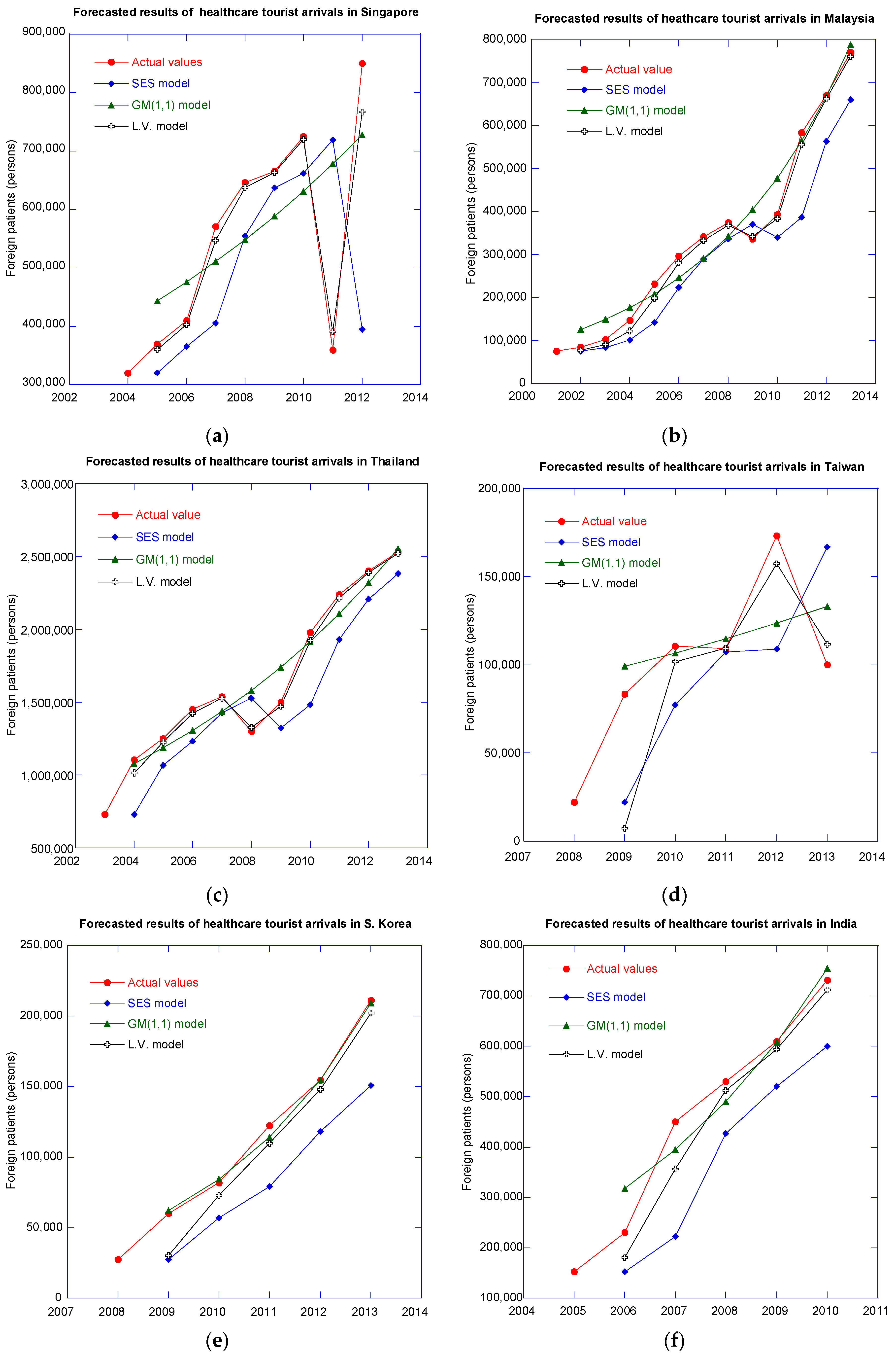
As shown in Table 1, the annual data of medical tourist arrivals for six destinations in Asia (Thailand, Singapore, Malaysia, Korea, Taiwan and India) were collected to conduct the forecast process. First, the total number of data points for individual destinations were utilized to build the forecast models. Then, to determine the forecast performance of different models in the healthcare traveling industry, model construction was conducted by the simple exponential smoothing model, the GM(1,1) model, and the L.V. model, respectively, for each destination. Finally, several statistical measurements of model errors and forecast precision (described in Section 3.4) have been used to analyze the performance of the proposed models.

The forecasted results have been calculated by the simple exponential smoothing model, the GM(1,1) model, and the L.V. model, and are reported in Figure 1. Forecasted curves and actual curves of medical tourist arrivals in individual destinations have been drawn. The forecasted performance of each forecast model was also evaluated and is shown in

Table 3. Performance of the proposed models for predicting the medical tourist arrivals in six destinations.

	Evaluative items	Maylaysia	Singapore	Thailand	Korea	Taiwan	India
Exponential Smoothing	MAD	191,682.06	157,220.89	669,091.67	32,907.03	45,471.7	125,534.9
	RMSE	293,201.8	218,369.8	1,058,751	37,672.3	51,854.5	136,711.7
	MAPE (%)	39.73	29.28	31.9	34.42	41.8	27.21
	Precision rate (%)	60.27	70.72	68.1	65.58	58.2	72.79
	Forecasting grade	Unqualified	Unqualified	Unqualified	Unqualified	Unqualified	Unqualified
GM(1,1) Model	MAD	39,040.55	113,545.53	115,834.49	2993.99	21,540.44	41,644.10
	RMSE	44,825.44	138,653.14	142,023.39	4068.66	27,664.76	50,930.88
	MAPE (%)	17.74	23.62	7.51	2.84	17.80	12.31
	Precision rate (%)	82.26	76.38	92.49	97.16	82.20	87.69
	Forecasting grade	Unqualified	Unqualified	Good	Excellent	Unqualified	Qualified
Lotka-Votterra Model	MAD	13,995.98	21,074.99	30,303.99	13,415.29	22,615.54	38,838.85
	RMSE	16,634.61	32,782.83	38,064.03	15,842.45	35,483.61	49,104.61
	MAPE (%)	6.03	3.61	2.10	15.87	24.10	10.10
	Precision rate (%)	93.97	96.39	97.90	84.13	75.90	89.90
	Forecasting grade	Good	Excellent	Excellent	Unqualified	Unqualified	Qualified

.

According to the results of the forecast performance of the three proposed models shown in Table 3, the error values of some measurements including the MAD, RMSE, and MAPE of the exponential smoothing model were clearly larger than the GM(1,1) model and the L.V. model, while these values of the GM(1,1) model were larger than the L.V. model. Particularly, the values of the error measurements of the exponential smoothing model fell from 669,091.67 to 32,907.03 for MAD value, from 1,058,751 to 37,672.3 for RMSE value and 41.8% to 27.21% for MAPE. Moreover, the precision rate of exponential smoothing ranged from 58.2% to 72.79%, and it did not reach the standard for reliable forecast as set by the classification grade of Ma and Zhang [44].

Similarly, the forecast performance of the GM(1,1) models were not better in this case. The values of MAD, RMSE, and MAPE of the GM(1,1) models were quite large, compared with the L.V. model. Thus, the forecast accuracy was much smaller, and the precision rate ranged from 82.2% to 97.17%. It was the only model to reach excellent forecast levels; one model achieved good forecast performance, and the other four GM(1,1) models had unqualified forecast performance.

In comparison with the previous two models, and based on the statistics of the error measures and the precision rate of the L.V. model as presented in Table 3, we realized that the L.V. models presented good forecast capability, with two models obtaining excellent forecast levels (96.39% and 97.9%), one model obtained good forecast levels (93.97%), one model presented a qualified forecast level (89.9%), and only two models (Korea and Taiwan) had unqualified forecast performances (75.9% and 84.69%). However, the forecast performance of these two cases by the GM(1,1) model was better than that of the L.V. model.

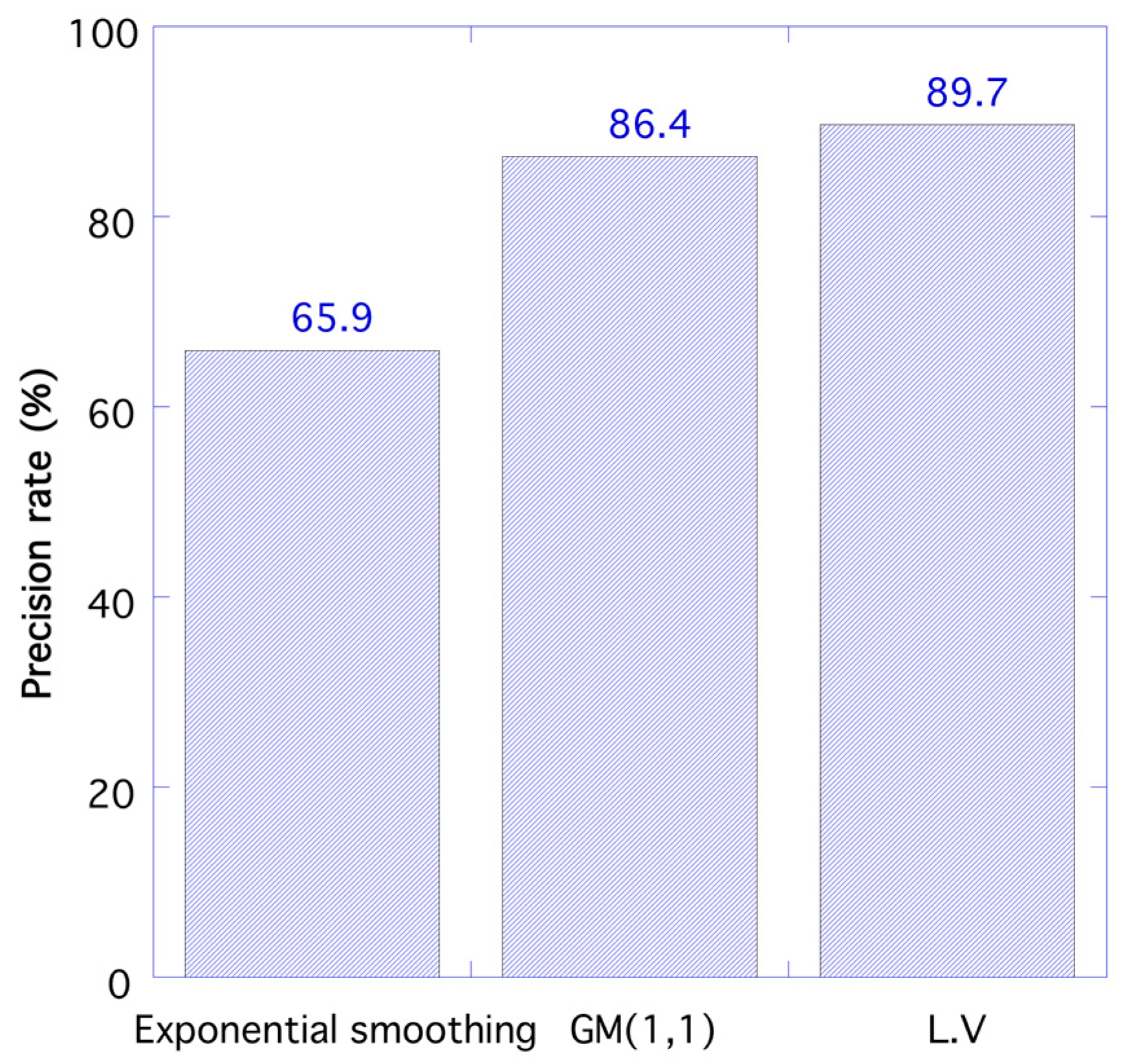
For making a clear and convenient comparison, we used the mean values of the precision rate in the six destinations to present the forecast performance of the three proposed models, shown in Figure 2.

Forecasted results from the 18 models indicated that the L.V. model had the best forecasted performance over the GM(1,1) model and the simple exponential smoothing model. According to Table 3, the values of some error measurements of the exponential smoothing model and the GM(1,1) were larger than the L.V. model. This means that the accuracy of the L.V. model was higher than the other two models. Generally, the mean precision rate of the L.V models was 89.7%, while that of the GM(1,1) models and exponential smoothing models was 86.36% and 65.94%, respectively.

The results proved that the L.V. models had higher prediction power than the traditional grey models and the exponential smoothing of traditional time series models under the same numerical data, and achieved the best forecasted performance among the three proposed models. Based on the empirical results, we suggest that the L.V. model can be used as an effective tool to estimate the future trend of medical tourist arrivals in the healthcare traveling industry. In contrast, the exponential smoothing model presented with inaccuracy for short-term forecasting with a small data size, so it is not suitable for use in this case. The forecasted performance of the GM(1,1) model was lower than the L.V. model, however its forecast level was still of a qualified grade. Therefore, besides the L.V. model, the GM(1,1) could be an alternative model for short-term forecasting with limited historical data.

5. Conclusions

Our research strengthens the prediction capability of forecasting models when using limited historical data. Based on the data of medical tourist arrivals, we applied three forecast models which did not require many historical data points for model construction, and these included the simple exponential smoothing model, the GM(1,1) model, and the L.V. model, to determine the forecast performance. The performance of proposed models was analyzed using the annual data of medical tourists in the healthcare traveling industry from 2001 to 2013 in six destinations (Thailand, Singapore, Malaysia, Korea, Taiwan and India) in Asia.

The results proved that the L.V. model had higher prediction power than the traditional grey model and the exponential smoothing model. It also presented the best forecasted performance among the three proposed models (89.7% precision rate). Based on the empirical results, we suggest that the L.V. model can be utilized as an effective tool to estimate the market size and identify the future trend of medical tourist arrivals in the healthcare traveling industry. Furthermore, although the forecasted performance of the GM(1,1) model was not better than the L.V. model, its accuracy level was still of a qualified grade (86.36% precision rate). Therefore, besides as the L.V. model, the GM(1,1) model can be an alternative for short-term forecasting with limited historical data. The exponential smoothing model was not appropriate for use in this case. The contribution of this study offers a useful statistical tool, which can be applied to the healthcare traveling industry in particular, and for other business forecasting as well, under the conditions of limited data in general. A good forecast can be obtained by using limited past data when using the right model.