Article

Feasibility Study on Parametric Optimization of Daylighting in Building Shading Design

1
School of Architecture, Hongik University, 94 Wausan-ro, Mapo-gu, Seoul 02481, Korea
2
Digit, 12, Dongmak-ro 2-gil, Mapo-gu, Seoul 04071, Korea
3
School of Architecture, University of Illinois at Urbana-Champaign, Champaign, IL 61820, USA
*
Authors to whom correspondence should be addressed.
Sustainability 2016, 8(12), 1220; https://doi.org/10.3390/su8121220
Submission received: 1 August 2016 / Revised: 20 October 2016 / Accepted: 18 November 2016 / Published: 24 November 2016
(This article belongs to the Section Sustainable Education and Approaches)

Abstract

:
Shading design to optimize daylighting is in many cases achieved through a designer’s sense based on prior knowledge and experience. However, computer-assisted parametric techniques can be utilized for daylighting design in an easy and much more accurate way. If such tools are utilized in the early stages of a project, this can be more effective for sustainable design. This study compares the conventional approach, which depends on a designer’s sense of judgment to create optimal indoor lighting conditions by adjusting louver shapes and window patterns, with the approach of making use of genetic algorithms. Ultimately, this study discusses the advantages and disadvantages of those two approaches. As a starting point, 30 designers were instructed to design a facade by manually adjusting several input parameters of shading. The parameters govern six kinds of louver and window types, with the ratio of analysis grid surface area achieving a daylight factor of 2%–5%. Secondly, input parameters were automatically created by using genetic algorithm optimization methods to find optimal fitness data. As a conclusion, conventional approaches result in a strong disposition toward designing certain shading types represented by linear relationships. Computer-assisted daylight simulation can help influence this, being effective when dealing with a large amount of data and non-linear relationships.

1. Introduction

The importance of sustainability in green building design is increasing. About 70% of all energy usage is consumed in urban areas, and lighting alone takes up around 15% of total building energy consumption [1,2,3]. Therefore, architects and engineers are actively looking for solutions to reduce lighting energy. Beside energy issues, lighting plays a significant role in buildings and urban areas more generally. Lighting, which can be divided into natural and artificial sources, can affect occupants’ comfort and satisfaction levels [4].
Inside a building, access to daylight makes the indoor environment healthier and more comfortable for occupants; natural lighting is also linked with greater productivity [5]. When designed with proper glare control and minimized solar heat gain, daylighting provides high-quality light while significantly reducing energy consumption for lighting and cooling. An effective facade shading design should contribute to the creation of such an environment that will reduce building energy expenditure and optimize daylight distribution [6,7,8].
There are several factors involved in the control of lighting energy, but the impact of the building skin on lighting is considerable. Formerly, architects typically designed the building skin based on previous experience and intuition. In order to achieve low-energy design, environmental engineers sometimes support the design by mathematical analysis. However, their involvement is often requested later in the design process. In the early design stages, passive design strategies can be optimized by considering an active design, which potentially improves the energy efficiency of buildings much more effectively [9,10,11,12]. Therefore, there is a need to integrate scientific methods with design to help a designer achieve low-energy design easily and effectively.
With the development of a design-integrated energy simulation, architects and designers can now more easily construct and design a building. Simulation programs which are combined with architectural daylighting design tools, such as DIVA-for-Grasshopper/Rhino were tested and used to design a building envelope [13]. With daylighting design, research-related building energy simulations such as Esp-r [14] or EnergyPlus [15] for energy-efficient buildings were also implemented in various areas. Furthermore, some simulation programs provide parametric methods or algorithms for optimization, which can help to find optimal solutions in a faster and easier way. Several pieces of research-related optimization techniques for transparent building facades [16] and genetic algorithms for design variables [17] show that those techniques can be an effective way to harmonize design and energy fields. Recently, utilizing digital technology based on computer hardware and software has been implemented in design projects, and this is known as parametric design [18,19]. Such technology can be actively and positively used in the early design stage for design optimization. For example, parametric modeling is related to geometric information which includes several parameters [20,21], and it can automatically modify parameters such as elevation proportion, louver size, and angle without reorganizing the whole model. Furthermore, other related research on energy performance of a building envelope and optimization of an engine or heat exchanger’s performance successfully adopts an optimization genetic algorithm [22,23,24], demonstrating how the application of a computer-aided algorithm has very important potential in architectural design.
In this study, other viewpoints and methods are introduced to clarify the distinction and importance compared to previous research. Above all, differences in daylighting between two design approaches will be tested: (A) design alternatives performed by an architectural designer’s experience and intuition; (B) design optimization by computer simulation will be tested. By comparing the architectural designer and the computer simulation, it can help to identify: (1) how much more daylighting performance a designer can achieve with a simulation program; (2) which louver and window types (defined as horizontal, vertical, random horizontal, random vertical louver types, and Delaunay and Voronoi screen types) can affect daylighting performance.
Secondly, this study explains how parametric optimization methods can be applied in daylighting design simulation. As a result, it can help to identify the advantages and disadvantages of daylighting optimization between designers and computer simulations. Also, this paper suggests how a designer’s manual and simulation methods can harmonize daylighting performance and facade design.
Architects design buildings through an iterative process using light simulation feedback. Light analysis can be simulated for either a simple or complex building facade. In other words, design processes are inseparable from simulations, to the extent that design can be controlled by the results of simulations. Thus, the main purpose of this research is to analyze and compare the uses of simulation results in buildings, specifically regarding the aspect of daylighting design. As a result, the processes of finding optimal solutions for daylighting design can be compared using a computer algorithm. Also, the proposed solutions can be tested on both a conventional envelope design as well as a computer-aided one, such as with Delaunay and Voronoi screens.

2. Methodology

2.1. Research Procedures and Methods

The main goal of this research is to find input parameters which can maximize fitness, i.e., the ratio of analysis grid surface area achieving a daylight factor (DF) of 2%–5% with variation of shape and combination of shading and window size in given conditions. This DF metric is a rather simplistic measure of daylighting performance, thus it is relatively easy to understand and be applied by an architectural designer in terms of simulation and analysis. The research was performed in the following three steps:
  • To find optimal fitness with manually input parameters adjusted by 30 persons,
  • To find optimal fitness data with Galapagos, a component inside Grasshopper that can optimize shape,
  • To find efficiency and improvement of optimization in green building facade design through a comparative analysis of manually adjusting input parameters and genetic algorithms.

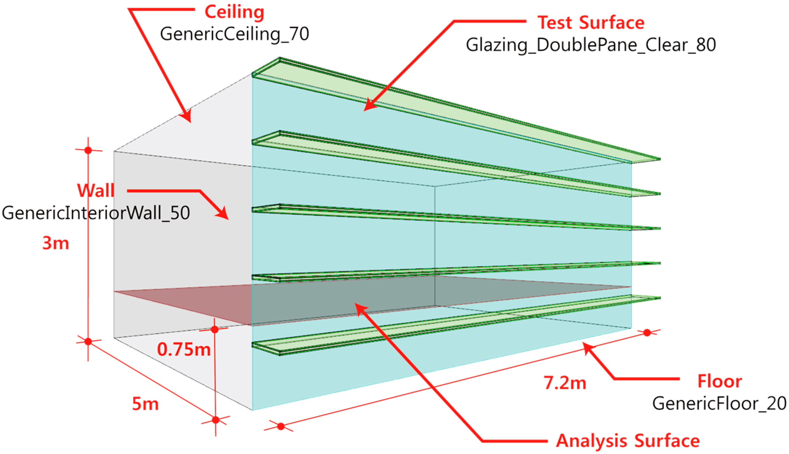
2.1.1. Base Simulation Model and Input Data

For simulation, a typical office space facing south is used as a base model, which measures 5 m (16.4 ft) depth by 7.2 m (23.6 ft) width, with a floor-to-floor height of 3 m (9.8 ft), as shown in Figure 1. South orientation was selected, which is most favorable, since there are no significant differences in DF by changes in orientation. Input materials for floor, wall, and ceiling were implemented as default values which are supported by DIVA in Table 1, and the selected glazing type is 8 mm double-pane clear glass.

2.1.2. Simulation Program and Basic Concept

As tools for parametric design and indoor lighting analysis, Grasshopper and DIVA are used [26]. Grasshopper is a graphical algorithm editor, a plug-in for Rhinoceros, a NURBS (Non-uniform rational B-spline curve) modeling software. It does not require knowledge of programming or scripting, and it allows designers to create simple to complex shapes. Once a definition for the Grasshopper is created, designers can easily adjust input parameter values and generate a variety of outputs for deformation and modification. Grasshopper is used for this experiment in order to easily adjust input parameters to find optimal fitness (output) manually. Using the Galapagos component, which is linked to those programs, an optimization method based on genetic algorithms in daylight fields can be applied using a personal computer.
DIVA-for-Grasshopper is a daylighting and energy modeling add-on for Grasshopper and an environmental simulation tool which can calculate data such as DF or solar irradiation parametrically. If it is done manually, people should adjust the value of the input parameters to find optimal fitness. When using Galapagos, associated input parameters execute an algorithm to automatically calculate the optimized output.

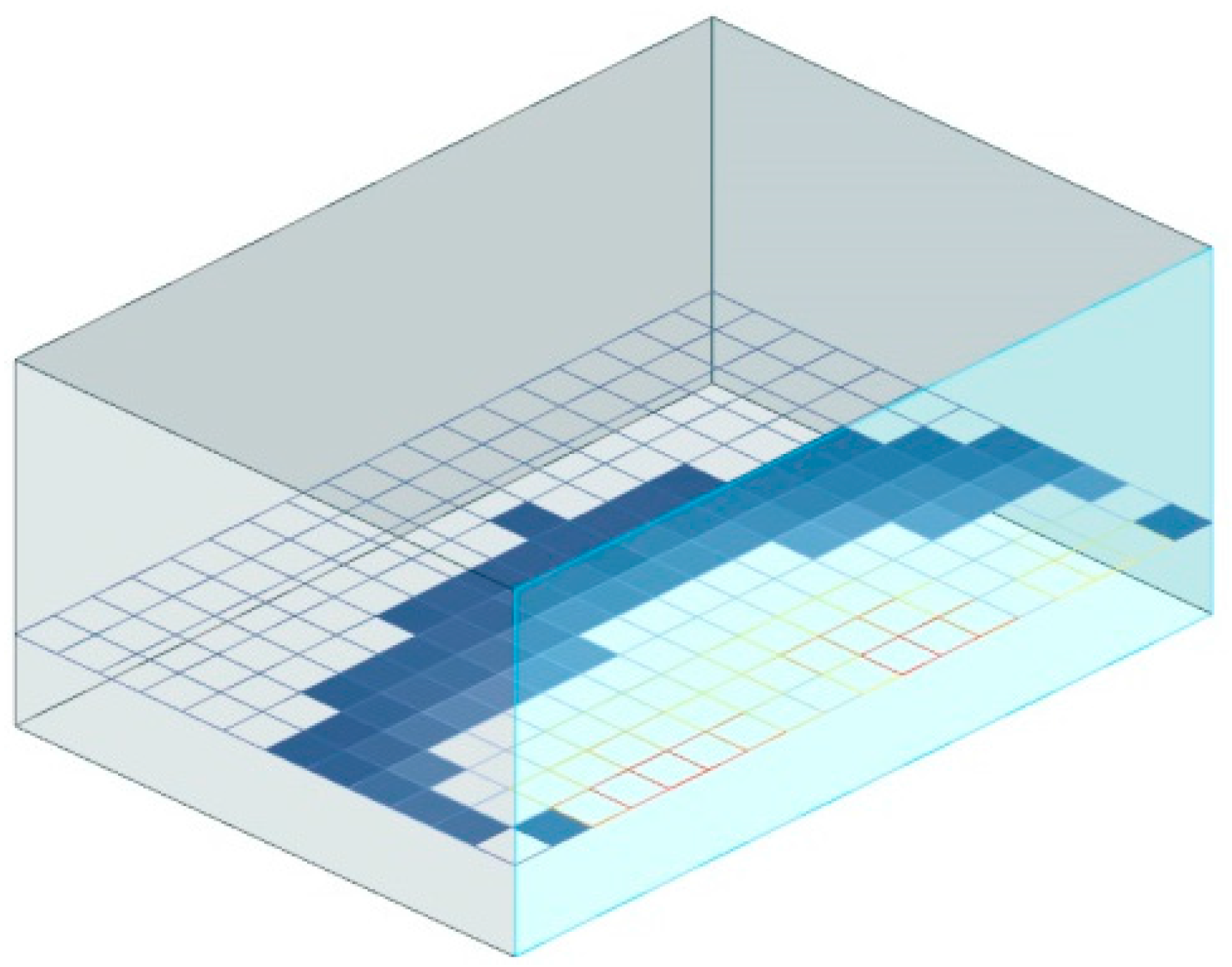
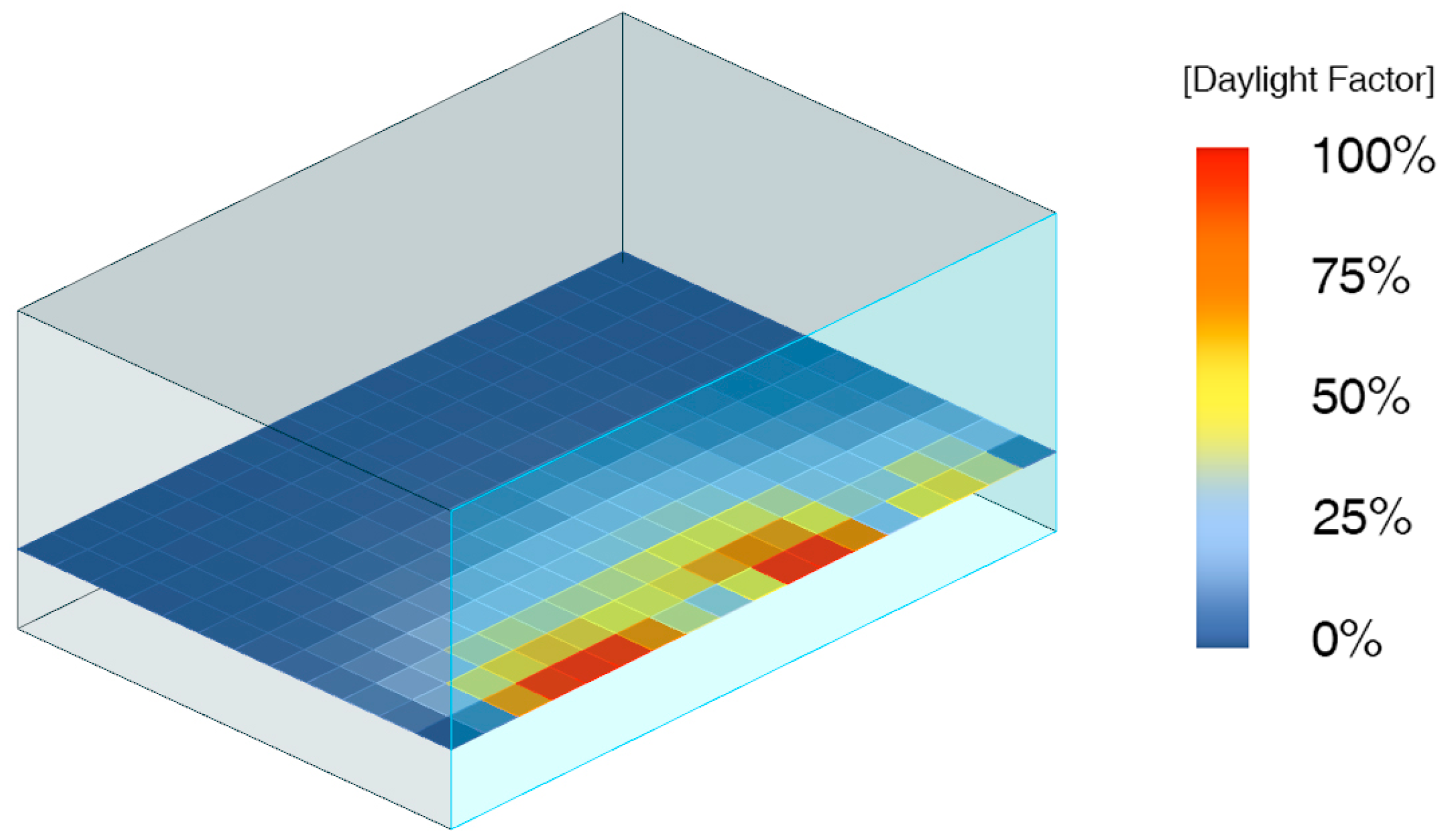
2.1.3. Daylight Factor (DF)

There are different types of metrics for daylighting. For instance, DF, daylight autonomy, and useful daylight illuminance are well-known metrics [7]. However, each metric comes with disadvantages as well as unique advantages. Daylight autonomy counts all the values over 300 lux, which is regarded as excessive light level. Also, useful daylight illuminance does not count any value over 2000 lux or below 100 lux. We have acknowledged those contradictory phenomena and have chosen DF for the research. Although it is not perfect, it is widely known and easy to understand. Even though the metrics are measured for either static or dynamic conditions, they are commonly considered static at a single point in time. In fact, the stability of DF is itself one of the benefits, regardless of the time of day or year, even assuming an overcast sky [27,28]. Also, DF is easy to calculate for buildings in the real world or models in the lab with illumination meters. Most European and Asian countries, such as the UK (BREEAM), France (HQE), Japan (CASBEE), and South Korea (G-SEED), use DF for green building assessment as part of their guidelines [29,30,31,32].
DF is a metric used to quantify the amount of diffuse daylight in a space. Diffuse daylight is light that has been scattered in the atmosphere before reaching the Earth’s surface. It is a ratio that represents the amount of illumination available indoors relative to the illumination present outdoors at the same time under an overcast sky. The design day for DF calculations is based on the standard International Commission on Illumination (CIE) overcast sky for 21 September at 12:00 p.m. [27,28]. It is usually measured at the height of the work plane (i.e., a desktop) under a standardized CIE overcast sky [33].
DF = (Ein/Eext) × 100
Ein: Interior illuminance at a fixed point on the work plane. Eext: Exterior illuminance under an overcast sky.
In the UK (CIBSE Lighting Guide 10), DF is categorized into three levels [34]:
(1)
DF under 2 is not adequately lit and artificial lighting will be required,
(2)
DF between 2 and 5 is adequately lit but artificial lighting may be in use for part of the time,
(3)
DF over 5 is well-lit and artificial lighting is generally not required except at dawn and dusk, although glare and solar gain may cause problems.
According to the British Standards Institution (BS 8206 part 2 CIBSE), a space with a mean DF between 2% and 5% is considered well-lit and requires little or no additional lighting during the day [35].
Also, the Indoor Environmental Quality in the LEED rating system recommends a 2% DF in at least 75% of all spaces occupied for critical visual tasks (LEED NC-v2.2 EQc8.1: Daylight and Views) [36].

2.1.4. Louver/Window Type and Input Parameters

In this experiment, louver and window types are formed from a combination of eight kinds of input parameters: (1). Angle: horizontal/vertical angle of the louver, from −60 to 60 degrees; (2). Num: number of louvers; (3). Depth: louver depth; (4). U Num.: number of window panel divisions in the horizontal direction; (5). V Num.: number of window panel divisions in the vertical direction; (6). WWR: window to wall ratio; (7). Pattern: Delaunay, Voronoi division pattern number (number of seed points of patterns); (8). Random: Delaunay, a random variable to be added to the Voronoi type. Each louver and window type has 125 variations with a combination of the three types of input parameters out of eight input parameters (Table 2). The parameters govern six kinds of louver and window types (horizontal, vertical, random horizontal, random vertical louver types, and Delaunay and Voronoi screen types) (Table 3 and Table 4).

2.2. Methods and Procedures of the Experiment

2.2.1. Manual Approach of Adjusting Input Parameters

Thirty students with at least four years of architectural design education participated in this experiment. They have fair understanding of Grasshopper and DIVA. They are also familiar with the concept of DF and indoor lighting environments through their sustainable architecture classes. The guidelines for the experiment are given as:
  • Adjust three parameters, and proceed with DIVA simulations. Check visual information of DF range being 2%–5% of the analysis grid surface area in the color index (Figure 2 and Figure 3).
  • Calculate the output (fitness: the ratio of analysis grid surface area having a DF value of 2% to 5%) as operation result.
  • Adjust the input parameters appropriately and choose the form of louvers which create a high fitness.
  • Check if three kinds of parameters are set properly using visual information of DF in the color index (Figure 2 and Figure 3). This assists participants in determining which parameter combination needs to be used for the next run and if the space needs more or less light.
  • Repeat at least 10 times for each window/louver type and adjust the input parameters in order to get to the highest possible optimal value.

2.2.2. Genetic Algorithm Optimization Methods Using Galapagos

Galapagos is used as the other experiment method to find optimum fitness values and three parameter values for each louver/window type using genetic algorithm optimization methods. The main reason why the genetic algorithm was selected is that it is the only algorithm to find optimal solutions with Rhino and Grasshopper software. In addition, this software is very widely used for architectural drawings [37]. In order to have equal conditions to those of manual methods, Galapagos is set with three parameter values with four variables: Max. Stagnant: 50, Population: 20, Maintain: 20%, Inbreeding: 50%. The Population, set as 20, means that evolution for each generation DIVA simulates 20 times. In this case, Max. Stagnant, set as 50, calculates up to 50 generations. The total number of simulations should be 1000, and the skip and filtering-method algorithm was programmed to avoid duplications. Stagnant by 20 of population. However, each louver/window type is composed with 125 cases in this research, and the maximum value of fitness could be found within ten generations.

3. Result

Table 5 shows the results of fitness (the ratio of analysis grid surface area having a DF value of 2% to 5%) by manual judgment against optimal fitness data from Galapagos. A total of 30 people ran the simulation, ten times for each louver or window type, to reach the highest fitness values. The average person’s data for each trial were compared, and the result (Table 5) includes the maximum and minimum of average, range, and standard deviation value from the average of the ten simulations. In order to compare the ratios to approach the maximum value for each type of louver or window under the same conditions, the original data need to be adjusted. The maximum fitness value for each type results from using Galapagos. Therefore, each type’s fitness is adjusted to 100 based on the Galapagos result for the comparison. Similarly, the other type’s fitness was also readjusted by applying the same ratio. The maximum of the average values for manual input ranges from 65% to 94%, and the minimum values of the average ranges from 32% to 87% compared to the optimization value by Galapagos. Among the six types, the vertical louver type reached the highest value (94%) by manual input, and the Voronoi screen type reached the lowest value (65%). The horizontal louver type has the highest average range (51%), and the random vertical and random horizontal louver type have the lowest average (3%). The average of the SD (standard deviation) of each trial ranges from 6 to 27. The horizontal louver type has the highest average of SD (27%) and the random vertical louver type has the lowest average of SD (6%). The maximum fitness value from the Galapagos optimization method ranges from 44% to 86%. The horizontal louver type has the highest value (86%), and the Voronoi screen type has the lowest value (44%). The minimum original fitness value from the Galapagos optimization method ranges from 0% to 36%.

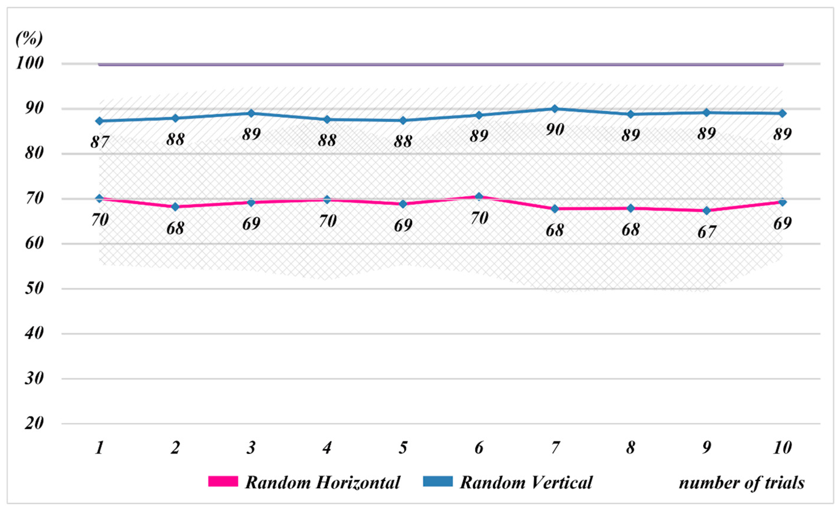
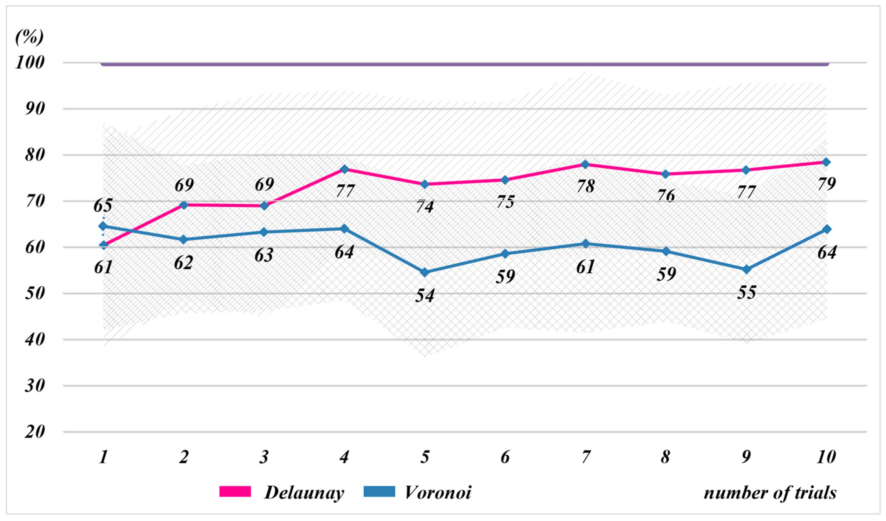
3.1. Manual Approach of Adjusting Input Parameters

The result of the experiment in which participants find optimal values by adjusting input parameters manually is illustrated in Figure 4, Figure 5 and Figure 6. Each graph shows the optimal value from 125 combinations of variables and the average value of ten tries by 30 participants. In the case of horizontal and vertical louver types, the more tries that are undertaken, the more optimal values are obtained (Figure 4). As an example, in the horizontal louver, the value of the first try was 36. This rose to 83 at the tenth try, which is an improvement of 2.3 times the original value. After ten repeated experiments, 83 was reached, which is 83% of the maximum value 86 from 125 combinations. In the vertical louver, the value of the first try was 76, which rose to 94 at the tenth try, which is an improvement of 1.2 times. After ten repeated experiments, 94 was reached, which is 94% of the maximum value 46 from 125 combinations. Participants learned the linear relationship between optimized output values and input parameters after repeated efforts. This test confirms that two types of louvers and windows are composed of linear input parameters, and the average value of 30 participants approaches the maximum value gradually. In other words, as the number of tries increases, participants become able to predict the results, and the most optimized facade design becomes possible. The minimum to maximum value of fitness spectrum of the horizontal louver type is larger than the vertical louver’s spectrum. It is interpreted that the combination of three input parameters influences the fitness values more critically in the horizontal louver type. The average values show that vertical is nearer the maximum value than horizontal. The basic fitness values are high regardless of input parameters. In addition, the variances of the horizontal louver are larger than those of the vertical louver, which is the unique characteristic of those louver types. As the louver is facing south in the base model of the experiment, daylight control of the horizontal louver is excellent compared to the vertical louver. Therefore, the weight of the horizontal louver is larger than the vertical louver for the input parameters.
However, the results of the random horizontal and random vertical with non-linear components remain steady regardless of the number of calculations (Figure 5). In the case of the random horizontal and random vertical, as the relationship between fitness and input parameters is non-linear, unlike the horizontal and vertical, the graph runs parallel to the x-axis. The random horizontal louver shows that the values of the first and tenth try are 70 and 69, respectively. The variance ranges from 67 minimum to 70 maximum overall. It only reaches 70% of 75, the maximum of 125 combinations. The random vertical louver shows that the difference between the first and tenth try is negligible, 87 for the first, and 89 for the tenth, respectively. Overall, the minimum value is 87 and the maximum is 90. However, it reaches 90% of 47, the maximum of 125 combinations. The reason is that the relationship between optimized output values and input parameters is unclear. Therefore, this unpredictability makes it difficult to improve fitness value toward the optimization. Due to irrelevancy, it is not useful when input parameters are adjusted manually.
Lastly, in the cases of the Delaunay and Voronoi screen types, which include non-linear components, the optimized values are not achievable since the relationship between optimized output values and input parameters are neither concrete nor predictable (Figure 6). The Delaunay screen type shows that the first try results in 61, and 79 occurs at the tenth try, which is an improvement of 1.3 times. After the tenth try, it reaches 79% of 47, the maximum value of 125 combinations. The Voronoi screen type indicates that the first try results in 65, while the tenth try gives a lower value of 64. When the unit sizes are compared between the Delaunay and Voronoi screen types, the Delaunay pattern has lower average values than the Voronoi pattern (Figure 7). The Delaunay pattern is more advantageous over the Voronoi pattern for the fact that subtle facade adjustment is possible and light is diffused evenly over the facade. Therefore, fitness values of the Delaunay screen type are larger than those of the Voronoi screen type.
As seen in Table 6, the statistical results of the previous six louver types were plotted. The horizontal and vertical louver types have relatively high R-squared value, 0.585 and 0.301, which indicates that those two types are on the regression line. The coefficient values of those two types seem to be significant by the p-value test, showing they have a much more linear relationship.

3.2. Genetic Algorithm Optimization Methods Using Galapagos

The results of using Galapagos for the six types of facades are as follows: The row on the left shows the input parameters’ combination of 125 cases (genome combination). The row on the right indicates the input parameters’ combination of the upper 10% fitness values (Figure 8).
The area with black dots on the left is a genome map (combination map). Each point refers to a gene (a parameter), and the distance between genes refers to a relationship. A genome (parameter combination) is made up of numerous genes. If a genome is decomposed into N genes, the distance count of two genes is N-dimensional, which means that all the cases are a count of “N raised to the power of N” [38].
It is impossible to render N-dimensional values with a two-dimensional plane. Therefore, this genome map only shows approximate relationships between genes. The definitive information on this map is how similar genes are, and how different they are. The relationship of genes is shown as the distance. If each point is grouped in a single point, it means that the number of combinations of parameters that make up the louver is less. However, if each point is distributed across multiple points, it means that there are fewer parameters of the combination of parameters to achieve the optimal illumination of the parameters, i.e., the optimized illumination environment.
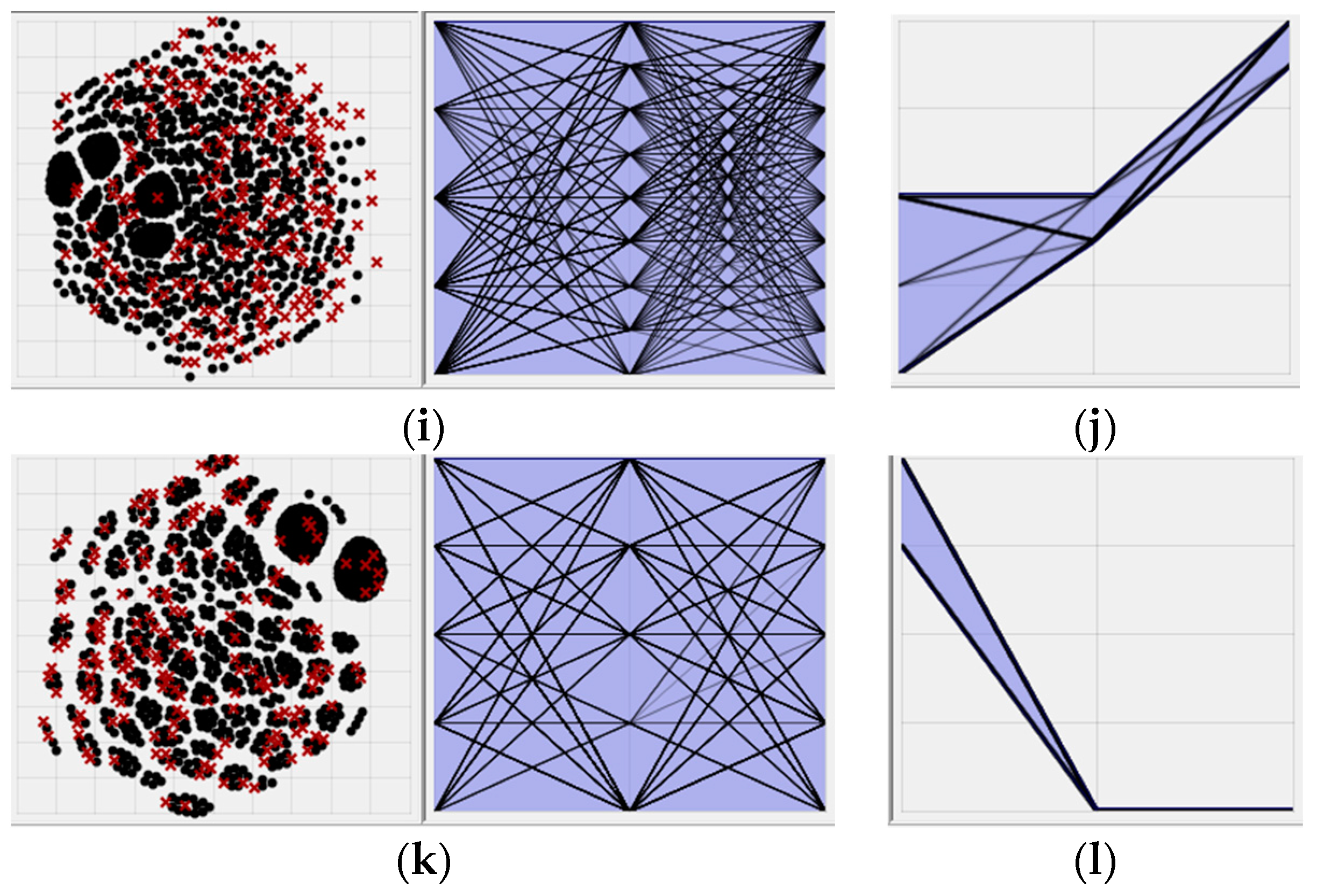
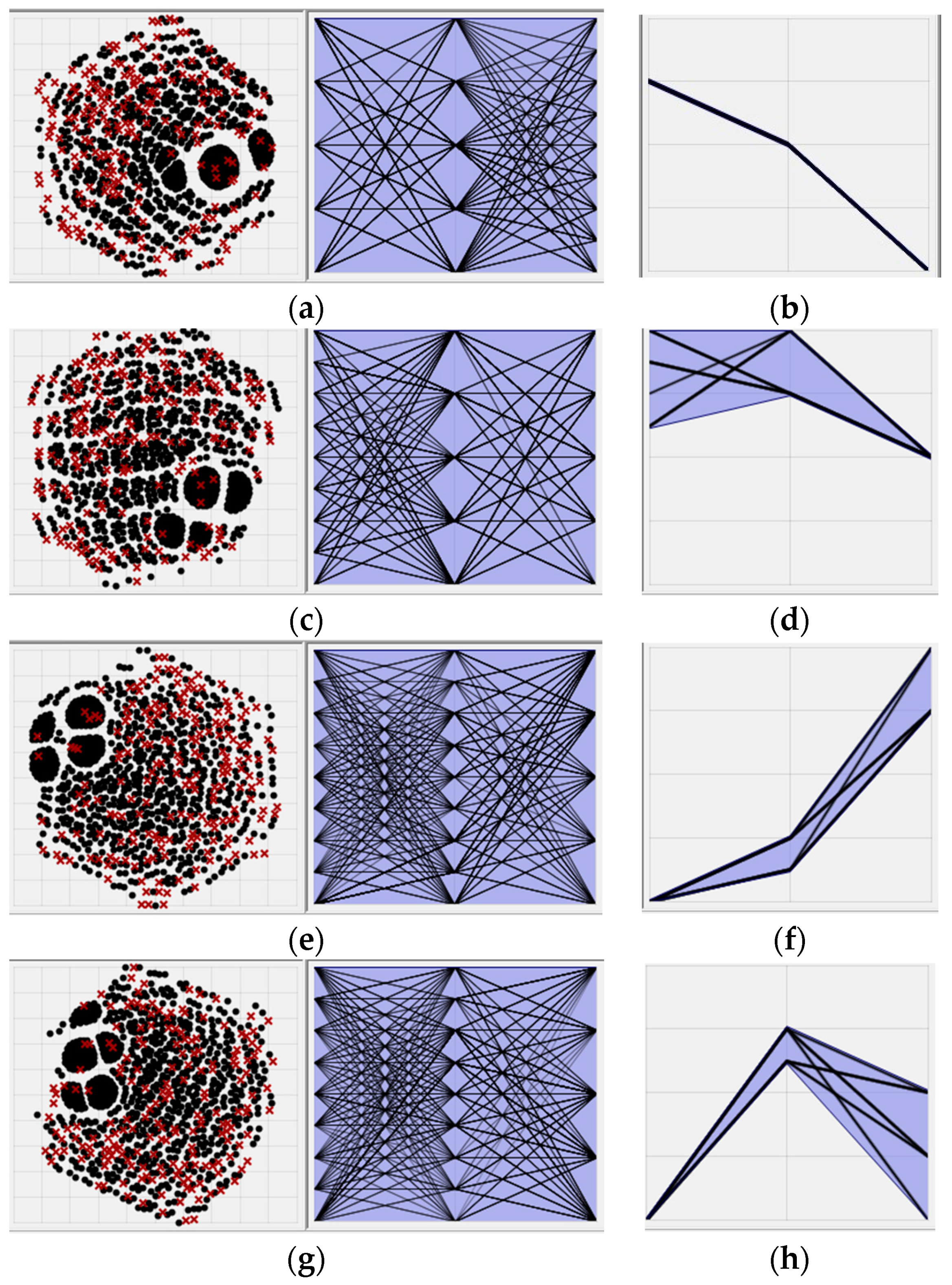
According to Figure 8, the horizontal axis is each parameter, i.e., count, angle, depth. The vertical axis is the number of cases (5 × 5 × 5) for each parameter. The upper 10% results for each type confirm the aggregation parts. It is apparent that the upper 10% fitness parameter combination gives only one kind in the case of the horizontal louver (Type 1) (Figure 8a). On the contrary, the different vertical louver types have diverse upper 10% fitness parameters. The random vertical louver (Figure 8h) provides six kinds of parameter combinations. In summary, the Galapagos results show that the random vertical louver has more design alternatives than the horizontal louver when it is set to find the upper 10% fitness values.

4. Conclusions

A feasibility study on parametric optimization of daylighting was performed, and the main findings can be summarized as follows:
  • Parametric design technology to create optimal indoor lighting conditions by adjusting shading shapes can help to improve daylighting quality in early design stages.
  • Conventional methods which depend on designers’ experience and knowledge can sufficiently be applied with computer simulation techniques in several design types, notably horizontal and vertical louver types, which represent linear relationships in daylight simulation.
  • Computer-assisted daylight simulation can help and assist the conventional approach, which can be maximized when dealing with large amounts of data and non-liner algorithms such as in the case of random, Delaunay, and Voronoi.
When the experiment is executed manually, it is possible to find the relationship between parameters and fitness. However, when the cases of parameter combination are large and complex, it takes considerable time to obtain the results, or sometimes it is difficult to reach optimal values. While the relationship between parameters and fitness is unobtainable using the genetic algorithms of Galapagos, it is effective to find the combination of parameters to reach a certain fitness value. In particular, it is useful when the number of parameters is large and the combination or algorithm is complex. Moreover, the optimization method using Galapagos provides various design alternatives in a scientific manner, which is executable on a personal computer. However, the downside is that the optimization method using Galapagos still needs the same amount of time even if the number of combinations is small. In that case, it is necessary to set population and generation values in Galapagos. The calculation continues until a certain number of calculations, i.e., population and generation, are reached. In other words, even if the combinations of parameters are found to produce the upper 10% or above of fitness, the calculation continues. Therefore, as seen in this experiment, when the total number of cases is only 125, it might be inefficient to use Galapagos. Nevertheless, the optimization method is useful for the fact that it is accessible without special skills or experience in daylighting design. A designer with insufficient knowledge of computer programming can apply facade design in a logical procedure. Instant views of results enable designers to develop their initial designs further, making Grasshopper a useful resource.
Currently, buildings are designed using computers and various software, as for daylighting. NURBS or randomized patterns which might have been hard to implement previously, can now be applied. Therefore, this research has revealed how those shading design methods are evaluated by comparing computer-aided simulations with conventional ones.

Acknowledgments

This research was supported by the Basic Science Research Program through the National Research Foundation of Korea (NRF) funded by the Ministry of Science, ICT & Future Planning (NRF-2014R1A1A1002268). Il Hyun Whang, a student of Hongik University, assisted in the collection of materials.

Author Contributions

Kyung Sun Lee and Jae Wook Lee conceived and designed the experiments; Ki Jun Han performed the experiments; Kyung Sun Lee and Jae Wook Lee analyzed the data; Ki Jun Han contributed analysis tools; Kyung Sun Lee and Jae Wook Lee wrote the paper.

Conflicts of Interest

The authors declare no conflict of interest.

Appendix A

Figure A1. The procedure for making the Delaunay pattern. (a) Selecting surface for analysis; (b) Selecting seed points (Pattern parameter, Random parameter); (c) Creating Delaunay pattern division; (d) Removing Delaunay cells by WWR parameter; (e) Application material: glass (80% visible transmittance)/wall (50% reflectance).
Sustainability 08 01220 g009aSustainability 08 01220 g009b
Figure A2. The procedure for making the Voronoi pattern. (a) Selecting surface for analysis; (b) Selecting seed points (Pattern parameter, Random parameter); (c) Creating Voronoi pattern division; (d) Removing Voronoi cells by WWR parameter; (e) Application material: glass (80% visible transmittance)/wall (50% reflectance).
Sustainability 08 01220 g010

References

  1. Lo, K. A critical review of China’s rapidly developing renewable energy and energy efficiency policies. Renew. Sustain. Energy Rev. 2014, 29, 508–516. [Google Scholar] [CrossRef]
  2. Deal, B.; Schunk, D. Spatial dynamic modeling and urban land use transformation: A simulation approach to assessing the costs of urban sprawl. Ecol. Econ. 2004, 51, 79–95. [Google Scholar] [CrossRef]
  3. Pérez-Lombard, L.; Ortiz, J.; Pout, C. A review on buildings energy consumption information. Energy Build. 2008, 40, 394–398. [Google Scholar] [CrossRef]
  4. Boubekri, M.; Hull, R.B.; Boyer, L.L. Impact of window size and sunlight penetration on office workers’ mood and satisfaction a novel way of assessing sunlight. Environ. Behav. 1991, 23, 474–493. [Google Scholar] [CrossRef]
  5. Boubekri, M. Daylighting, Architecture and Health; Routledge: Abingdon, UK, 2008. [Google Scholar]
  6. Boyce, P.; Hunter, C.; Howlett, O. The Benefits of Daylight through Windows; Rensselaer Polytechnic Institute: Troy, NY, USA, 2003. [Google Scholar]
  7. Reinhart, C.F.; Mardaljevic, J.; Rogers, Z. Dynamic daylight performance metrics for sustainable building design. Leukos 2006, 3, 7–31. [Google Scholar]
  8. Munaaim, M.A.C.; Al-Obaidi, K.M.; Ismail, M.R.; Rahman, A.M.A. Empirical evaluation of the effect of heat gain from fiber optic daylighting system on tropical building interiors. Sustainability 2014, 6, 9231–9243. [Google Scholar] [CrossRef]
  9. Lee, K.S.; Lee, J.; Lee, J.S. Low-energy design methods and its implementation in architectural practice: Strategies for energy-efficient housing of various densities in temperate climates. J. Green Build. 2013, 8, 164–183. [Google Scholar] [CrossRef]
  10. Augenbroe, G. Integrated building performance evaluation in the early design stages. Build. Environ. 1992, 27, 149–161. [Google Scholar] [CrossRef]
  11. Cheong, C.H.; Kim, T.; Leigh, S.B. Thermal and daylighting performance of energy-efficient windows in highly glazed residential buildings: Case study in Korea. Sustainability 2014, 6, 7311–7333. [Google Scholar] [CrossRef]
  12. Piderit Moreno, M.B.; Labarca, C.Y. Methodology for Assessing Daylighting Design Strategies in Classroom with a Climate-Based Method. Sustainability 2015, 7, 880–897. [Google Scholar] [CrossRef]
  13. Jakubiec, J.A.; Reinhart, C.F. DIVA 2.0: Integrating daylight and thermal simulations using Rhinoceros 3D, Daysim and EnergyPlus. In Proceedings of Building Simulation 2011: 12th Conference of International Building Performance Simulation Association, Sydney, Australia, 14–16 November 2011; Volume 20, pp. 2202–2209.
  14. Bourgeois, D.; Reinhart, C.; Macdonald, I. Adding advanced behavioural models in whole building energy simulation: A study on the total energy impact of manual and automated lighting control. Energy Build. 2006, 38, 814–823. [Google Scholar] [CrossRef]
  15. Crawley, D.B.; Lawrie, L.K.; Winkelmann, F.C.; Buhl, W.F.; Huang, Y.J.; Pedersen, C.O.; Glazer, J. EnergyPlus: Creating a new-generation building energy simulation program. Energy Build. 2001, 33, 319–331. [Google Scholar] [CrossRef]
  16. Lee, J.W.; Jung, H.J.; Park, J.Y.; Lee, J.B.; Yoon, Y. Optimization of building window system in Asian regions by analyzing solar heat gain and daylighting elements. Renew. Energy 2013, 50, 522–531. [Google Scholar] [CrossRef]
  17. Caldas, L.G.; Norford, L.K. A design optimization tool based on a genetic algorithm. Autom. Constr. 2002, 11, 173–184. [Google Scholar] [CrossRef]
  18. Iqbal, I.; Al-Homoud, M.S. Parametric analysis of alternative energy conservation measures in an office building in hot and humid climate. Build. Environ. 2007, 42, 2166–2177. [Google Scholar] [CrossRef]
  19. Attia, S.; Gratia, E.; De Herde, A.; Hensen, J.L. Simulation-based decision support tool for early stages of zero-energy building design. Energy Build. 2012, 49, 2–15. [Google Scholar] [CrossRef]
  20. Ward, G.; Shakespeare, R. Rendering with Radiance: The Art and Science of Lighting Visualization; Morgan Kaufmann Publishers: Burlington, MA, USA, 1998. [Google Scholar]
  21. Blackwell, O.M.; Blackwell, H.R. Individual responses to lighting parameters for a population of 235 observers of varying ages. J. Illum. Eng. Soc. 1980, 9, 205–232. [Google Scholar] [CrossRef]
  22. Ascione, F.; Bianco, N.; de Masi, R.F.; Mauro, G.M.; Vanoli, G.P. Design of the building envelope: A novel multi-objective approach for the optimization of energy performance and thermal comfort. Sustainability 2015, 7, 10809–10836. [Google Scholar] [CrossRef]
  23. Sadeghzadeh, H.; Aliehyaei, M.; Rosen, M.A. Optimization of a Finned Shell and Tube Heat Exchanger Using a Multi-Objective Optimization Genetic Algorithm. Sustainability 2015, 7, 11679–11695. [Google Scholar] [CrossRef]
  24. Turkson, R.F.; Yan, F.; Ali, M.K.A.; Liu, B.; Hu, J. Modeling and multi-objective optimization of engine performance and hydrocarbon emissions via the use of a computer aided engineering code and the NSGA-II genetic algorithm. Sustainability 2016, 8, 72. [Google Scholar] [CrossRef]
  25. IES Daylight Metrics Committee. IES Spatial Daylight Autonomy (sDA) and Annual Sunlight Exposure (ASE), Daylight Metrics Committee. Approved Method IES LM-83-12; Illuminating Engineering Society of North America: New York, NY, USA, 2012. [Google Scholar]
  26. Website of Solemma. Available online: http://www.solemma.net/DIVA-for-Rhino/DIVA-for-Rhino.html (accessed on 14 October 2016).
  27. Ismail, E.D.; Ibrahim, N.; Hajar, N.H. Daylight Factor on Natural Lighting Analysis Simulation of an Adaptive Reuse Building: Penaga Hotel, Penang. Adv. Sci. Lett. 2016, 22, 1120–1124. [Google Scholar] [CrossRef]
  28. Galatioto, A.; Beccali, M. Aspects and issues of daylighting assessment: A review study. Renew. Sustain. Energy Rev. 2016, 66, 852–860. [Google Scholar] [CrossRef]
  29. Building Research Establishment. BREEAM—The BRE Environmental Assessment Method. Available online: http://www.breeam.org (accessed on 12 October 2016).
  30. Kudryashova, A. Certification Schemes for Sustainable Buildings: Assessment of BREEAM, LEED and LBC from a Strategic Sustainable Development Perspective. Ph.D. Thesis, Blekinge Institute of Technology, Blekinge, Sweden, 2015. [Google Scholar]
  31. Lim, Y.W. Building Information Modeling for Indoor Environmental Performance Analysis. Am. J. Environ. Sci. 2015, 11, 55–61. [Google Scholar] [CrossRef]
  32. CASBEE for Building (New Construction). 2014 Edition. Available online: http://www.ibec.or.jp/CASBEE/english/ (accessed on 12 October 2016).
  33. Day Lighting Rules of Thumb. Available online: http://www.gsd.harvard.edu/research/gsdsquare/Publications/DiffuseDaylightingDesignSequenceTutorial.pdf (accessed on 12 December 2015).
  34. CIBSE Lighting Guide. 10: Daylighting and Window Design; The Chartered Institution of Building Services Engineers: London, UK, 1999. [Google Scholar]
  35. British Standards Institution. Available online: http://www.cibse.org/pdfs/GPG245.pdf (accessed on 5 January 2016).
  36. LEED for New Construction & Major Renovations. Available online: http://www.usgbc.org/Docs/Archive/General/Docs1095.pdf (accessed on 8 February 2016).
  37. Yi, Y.K.; Kim, H. Agent-based geometry optimization with Genetic Algorithm (GA) for tall apartment’s solar right. Sol. Energy 2015, 113, 236–250. [Google Scholar] [CrossRef]
  38. Rutten, D. Galapagos: On the logic and limitations of generic solvers. Arch. Des. 2013, 83, 132–135. [Google Scholar] [CrossRef]
Figure 1. Base model.
Sustainability 08 01220 g001
Figure 2. Analysis grid surface of DF range between 2% to 5%.
Sustainability 08 01220 g002
Figure 3. Analysis grid surface of DF.
Sustainability 08 01220 g003
Figure 4. Horizontal louver vs. Vertical louver.
Sustainability 08 01220 g004
Figure 5. Random horizontal louver vs. Random vertical louver.
Sustainability 08 01220 g005
Figure 6. Delaunay screen type vs. Voronoi screen type.
Sustainability 08 01220 g006
Figure 7. Unit size variation by panel division of Delaunay window screen vs. Voronoi screen type.
Sustainability 08 01220 g007
Figure 8. Galapagos results. (a) Horizontal louver (Type 1); (b) Horizontal louver (Type 1)—Top 10%; (c) Vertical louver (Type 2); (d) Vertical louver (Type 2)—Top 10%; (e) Random horizontal (Type 3); (f) Random horizontal (Type 3)—Top 10%; (g) Random vertical louver (Type 4); (h) Random vertical louver (Type 4)—Top 10%; (i) Delaunay pattern (Type 5); (j) Delaunay pattern (Type 5)—Top 10%; (k) Voronoi pattern screen; (l) Voronoi pattern screen—Top 10%.
Sustainability 08 01220 g008aSustainability 08 01220 g008b
Table 1. Combination of input parameters for louver/window type.
Input MaterialsMaterial Name in DIVAMaterial Properties
1WallGenericInteriorWall_50This is a purely diffuse reflector with a standard wall reflectivity of 60%
2CeilingGenericCeiling_70Material for typical ceilings as suggested by IES-LM-83 [25]
3WindowGlazing_DoublePane_Clear_80Visual transmittance: 80%
Visual transmissivity: 87%
4FloorGenericFloor_20This is a purely diffuse reflector with a standard floor reflectivity of 20%
Table 2. Input parameters.
Input ParametersUnitRange (min.)Range (max.)Step SizeVariables
1Angle (degree)Horizontal/vertical angle adjustment of the louver−6060305
2Num. (integer)The number of louvers51325
3Depth (10 cm)Louver depth2615
4U Num. (integer)Number of window panel divisions in the U direction51325
5V Num. (integer)Number of window panel divisions in the V direction51325
6Remove (-)Ratio of remove from the entire window panel0.2 (20%)0.8 (80%)0.15 (15%)5
7Pattern (step)Number of seed point patterns1050105
8Random (-)Random variable for seed points 1515
Table 3. Combination of input parameters for louver/window types.
12 3 4 56
Input ParametersHorizontal LouverVertical LouverRandom Horizontal LouverRandom Vertical LouverDelaunay Pattern ScreenVoronoi Pattern Screen
1Angle----
2Num.----
3Depth----
4U Num.----
5V Num.----
6Remove--
7Pattern----
8Random----
No. total variations125125125125125125
√: Applied parameters.
Table 4. Louver/window types.
(a) Horizontal louver
Parameters: Angle, Num., Depth
(b) Vertical louver
Parameters: Angle, Num., Depth
Sustainability 08 01220 i001 Sustainability 08 01220 i002
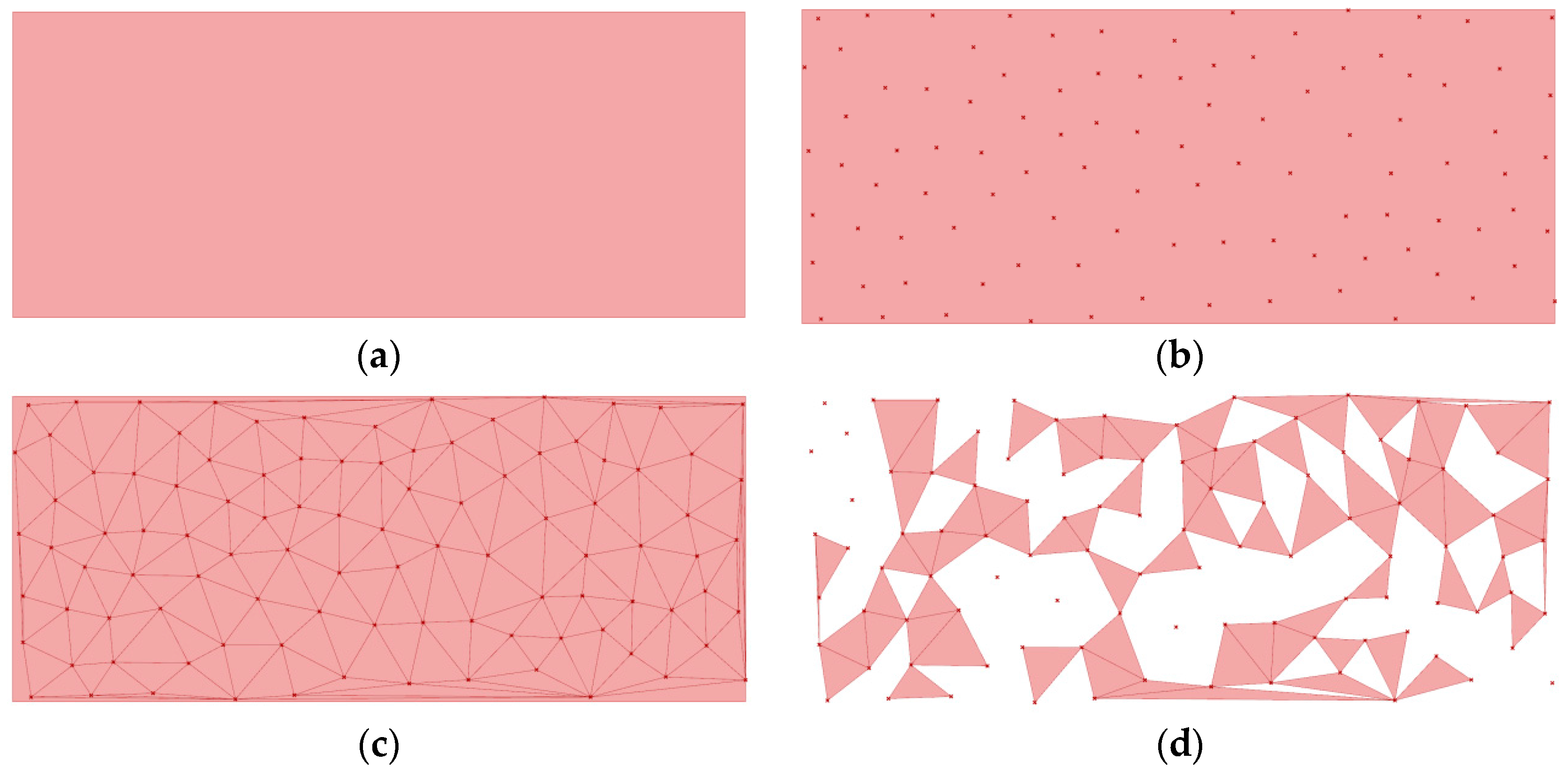
(c) Random horizontal louver
Parameters: U Num., V Num., WWR
(d) Random vertical louver
Parameters: U Num., V Num., WWR
Sustainability 08 01220 i003 Sustainability 08 01220 i004
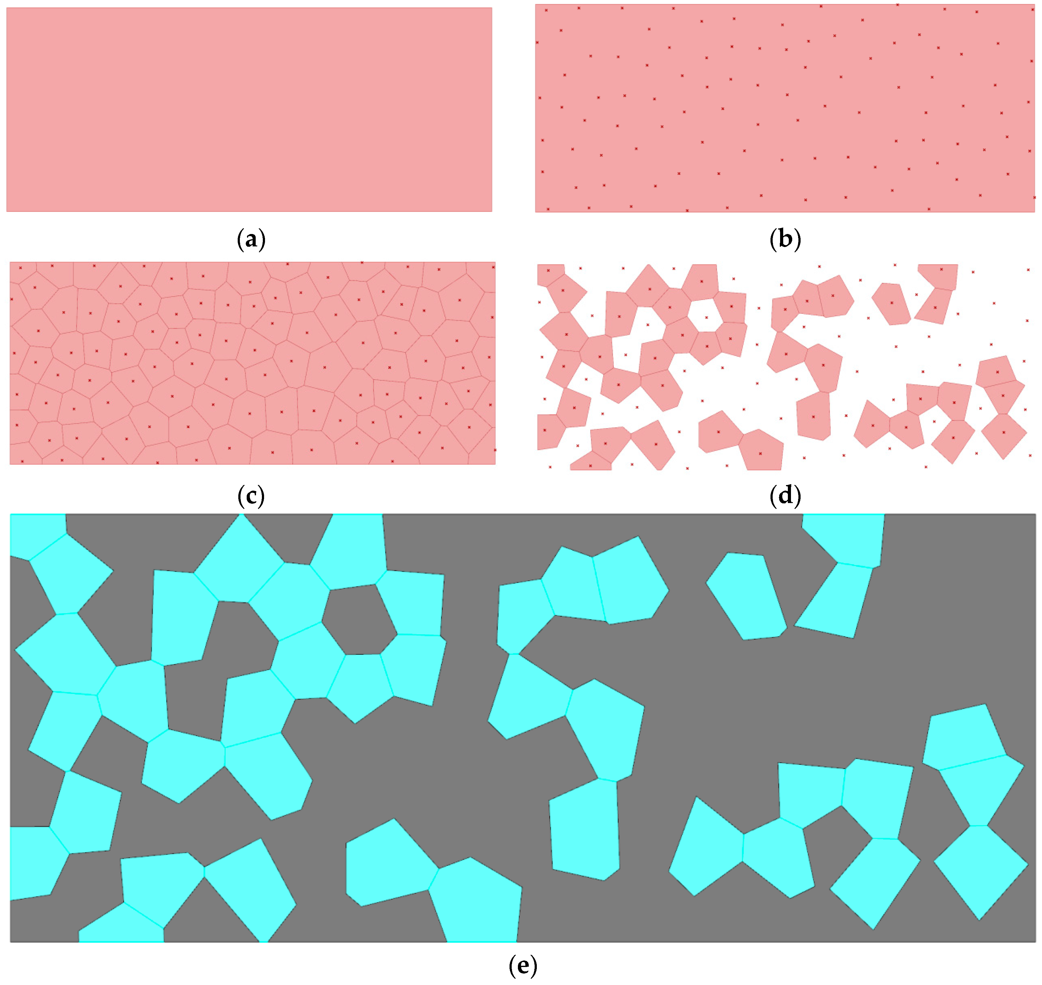
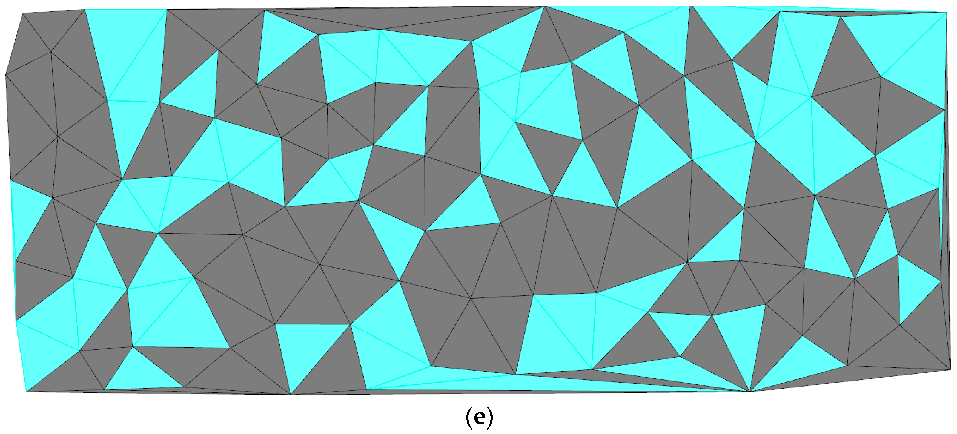
(e) Delaunay pattern screen (Figure A1) *
Parameters: WWR, Pattern, Random
(f) Voronoi pattern screen (Figure A2) *
Parameters: WWR, Pattern, Random
Sustainability 08 01220 i005 Sustainability 08 01220 i006
Green: Solid wall; Blue: Window glass. * The detailed procedures described in Figures are found in Appendix A.
Table 5. Statistical data from manual input vs. Galapagos program.
MethodManual Approach (Adjusted Data)Galapagos (Original Data)
Fitness Value (%)Max. of Avg.Min. of Avg.Aver. SDMax. Min.
Louver/WindowType Parameter Value
Horizontal
(Type 1)
833227860
0/5/5
Vertical
(Type 2)
947694626
0/11/6, 0/13/0
Random horizontal
(Type 3)
7067167520
5/11/0.35
Random vertical
(Type 4)
908764736
11/5/0.2
Delaunay
(Type 5)
796119476
0.65/30/2
Voronoi
(Type 6)
655518440
0.2/10/4, 0.2/10/5
Table 6. Statistical results of the six louver/window types.
TypeCoefficientsConstant(S.E.)p-Value
Horizontal
R-squared: 0.585
5.71 **23.04(0.28)0.001
Vertical
R-squared: 0.301
1.96 **73.71(0.17)0.001
Random horizontal
R-squared: 0.001
−0.1469.60(0.32)0.65
Random vertical
R-squared: 0.008
0.1987.57(0.12)0.12
Delaunay
R-squared: 0.049
1.53 **64.93(0.39)0.001
Voronoi
R-squared: 0.006
−0.4763.10(0.36)0.19
**: p < 0.01.

