Article

The Dynamic Enterprise Network Composition Algorithm for Efficient Operation in Cloud Manufacturing

1
Department of Industrial and Management Engineering, Hanyang University, Ansan 15588, Korea
2
School of Business Administration, College of Business and Economics, Chung-Ang University, Seoul 06974, Korea
*
Author to whom correspondence should be addressed.
Sustainability 2016, 8(12), 1239; https://doi.org/10.3390/su8121239
Submission received: 14 October 2016 / Revised: 7 November 2016 / Accepted: 23 November 2016 / Published: 29 November 2016
(This article belongs to the Special Issue Sustainability in Supply Chain Management)

Abstract

:
As a service oriented and networked model, cloud manufacturing (CM) has been proposed recently for solving a variety of manufacturing problems, including diverse requirements from customers. In CM, on-demand manufacturing services are provided by a temporary production network composed of several enterprises participating within an enterprise network. In other words, the production network is the main agent of production and a subset of an enterprise network. Therefore, it is essential to compose the enterprise network in a way that can respond to demands properly. A properly-composed enterprise network means the network can handle demands that arrive at the CM, with minimal costs, such as network composition and operation costs, such as participation contract costs, system maintenance costs, and so forth. Due to trade-offs among costs (e.g., contract cost and opportunity cost of production), it is a non-trivial problem to find the optimal network enterprise composition. In addition, this includes probabilistic constraints, such as forecasted demand. In this paper, we propose an algorithm, named the dynamic enterprise network composition algorithm (DENCA), based on a genetic algorithm to solve the enterprise network composition problem. A numerical simulation result is provided to demonstrate the performance of the proposed algorithm.

1. Introduction

As consumer demand has changed drastically and quickly, mass customization to deal with the customers’ demands has been popular in manufacturing. The main goal is to provide customized products or services effectively and efficiently, in terms of customer’s specified needs at reasonable prices [1]. It is essential for an enterprise to retain various manufacturing resources, such as design, production, testing, and logistic resources, while being able to change the kinds, and the amounts, of resources in accordance with the demands of customers for realization of mass customization. Unfortunately, it is impossible for an enterprise, especially for small and medium-sized enterprises (SMEs), to retain all of these manufacturing resources, or change the amount of resources to satisfy all of the requirements of customers. This is why mass customization has largely not lived up to its promised potential [2].
Sharing manufacturing resources among multiple enterprises may be a solution to realize mass customization, but it has been difficult to cooperate and share resources among enterprises because existing manufacturing models have been constructed independently of other enterprises and, as a result, they cannot share the resources efficiently. For this reason, a new integrated manufacturing model based on cloud computing technology, called cloud manufacturing (CM), has been proposed more recently [3]. Owing to cloud computing technology that enables ubiquitous and on-demand network access to a shared pool of configurable computing resources [4], CM can provide a shared manufacturing resource pool that can be managed and operated in a unified and intelligent way.
In this sense, various enterprises participating in CM can share manufacturing resources and cooperate with each other to produce highly-customized manufacturing services even though the services are too large or too complex to handle for one enterprise [5]. In addition, CM can deliver reliable, high-quality, and on-demand manufacturing services for the whole lifecycle of manufacturing, such as design, production, testing, and logistics [6], by enabling the enterprises to freely access every manufacturing service in the manufacturing cloud (MC), without certain expertise in the management of resources used. That is, MC is a main component of cloud manufacturing to utilize the manufacturing process in CM. Thus, we use the terms CM and MC separately to distinguish the manufacturing model (CM) and platform (MC), clarifying the manufacturing process in CM. The MC is a manufacturing platform made up of universal and renewable manufacturing resources with flexibility [
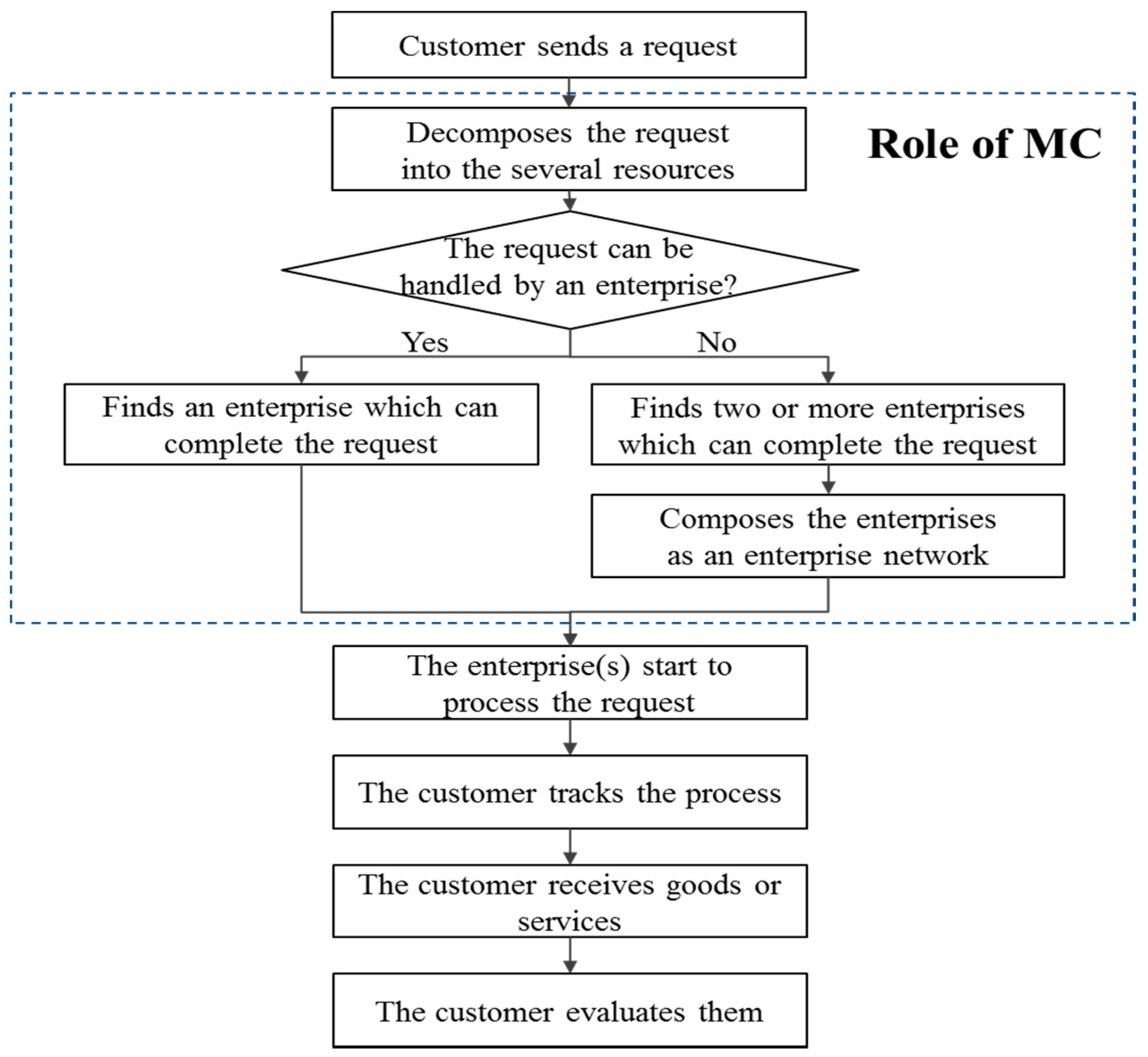
7]. In the MC, diversified manufacturing resources can be intelligently sensed and connected into the wider Internet, and automatically managed and controlled by means of the Internet of Things (IoT) and related technologies (e.g., radio frequency identification (RFID), wireless sensor network, embedded system, etc.). Then those are virtualized and encapsulated into the MC, which means they are enrolled in the MC with identification factors (e.g., name, inventory level, location). They can be accessed, invoked, and deployed by means of cloud computing technologies, virtualization technologies, and service-oriented technologies after that. MC automatically analyzes customers’ requests to estimate the required resources and the amount of them to complete the requests. After the estimation, MC finds the appropriate enterprise(s) that could successfully complete the request. If the request is so large that two or more enterprises are needed to complete the request, then MC composes the enterprise network for the request. The formal operation process to complete a customer request in MC is presented in Figure 1. As seen in Figure 1, if the request is too large for an enterprise to complete it (e.g., the request requires various resources or a lot of resources), MC finds and selects two or more enterprises and composes a network of enterprises [8].
Cloud manufacturing is defined by many researchers: Xu [9] defined CM as “a model for enabling ubiquitous, convenient, on-demand network access to a shared pool of configurable manufacturing resources (e.g., manufacturing software tools, manufacturing equipment, and manufacturing capabilities) that can be rapidly provisioned and released with minimal management effort or service provider interaction”. Meanwhile, Wu et al. [10] defined CM as a “customer-centric manufacturing model that exploits on-demand access to a shared collection of diversified and distributed manufacturing resources to form temporary, reconfigurable production lines which enhance efficiency, reduce product lifecycle costs, and allow for optimal resource loading in response to variable-demand customer generated tasking”.
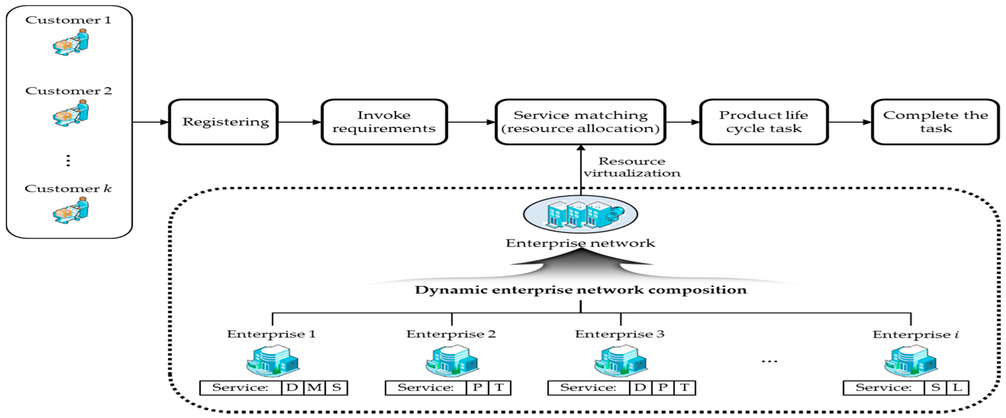
Figure 2 illustrates the whole life cycle process of CM [11]: First of all, enterprises contract with CM and participate in CM. This contract generates the participation contract cost. Once the enterprise takes part in CM, it is possible to collect the resource information of each enterprise, such as the amount of resources the enterprise currently reserves, which is virtualized and encapsulated in the MC. Customers participating in CM invoke requirements about the products or services they want and the requirements are reorganized to be recognized as demands in CM. Types of resources, due dates, the amount of resources, and so forth, are included in the requests. After that, customer demands are matched with the adequate manufacturing service in the MC considering the information about the resource capabilities of each enterprise. The type of matching requirements and services could be either one-to-one (one enterprise is assigned to the service of one customer), N-to-one (two or more enterprises are assigned to the service of one customer), one-to-N (one enterprise is assigned to the service of two or more customers), or N-to-N (two or more enterprises are assigned to the service of two or more customers). N enterprises compose a temporary production network for one-to-N and N-to-N cases, while there is no need to compose the network for one-to-one and N-to-one cases. Finally, some enterprises in CM may leave CM, which generates a contract cancellation cost.
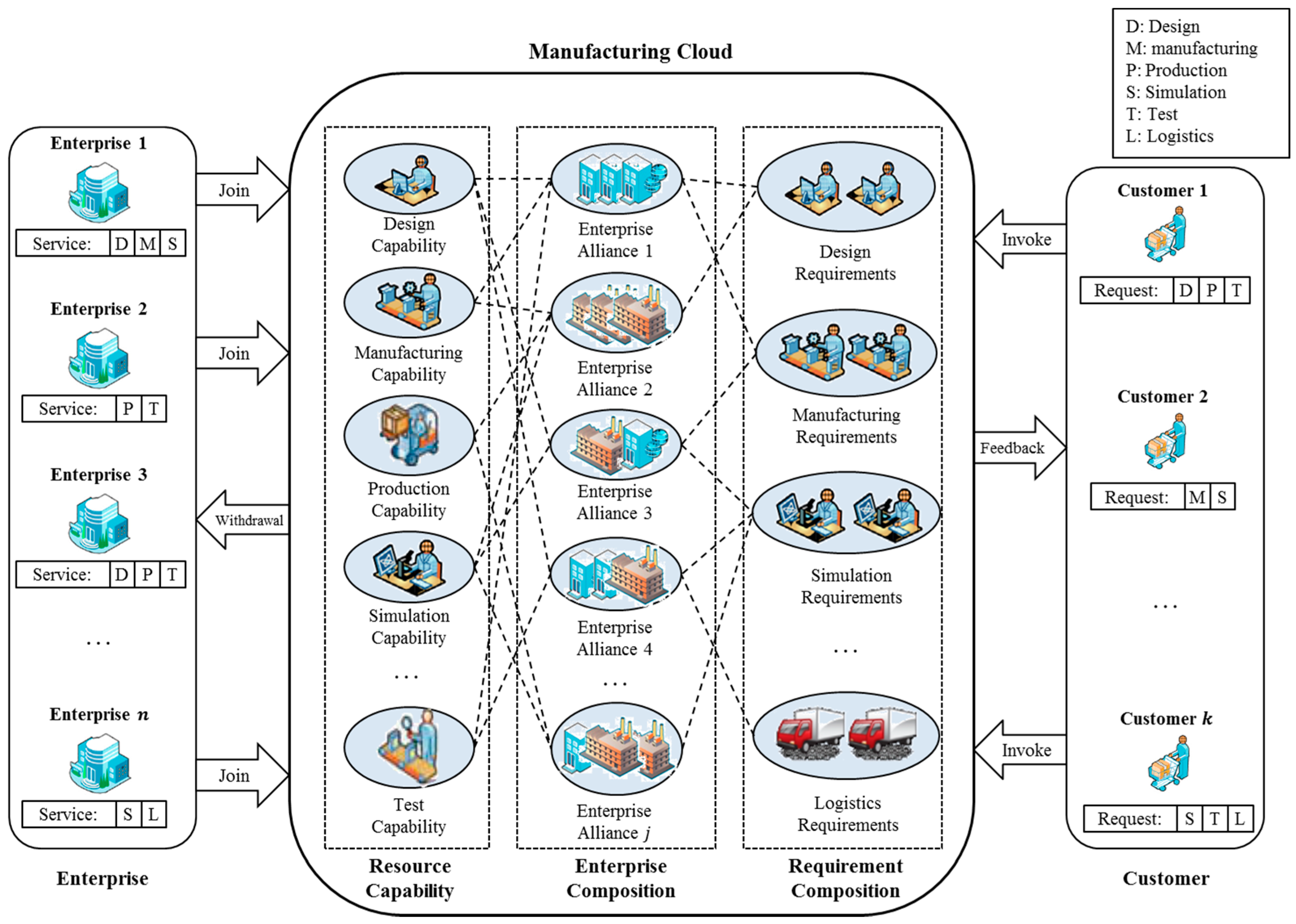
As an example of the operation process, suppose enterprises 1, 2, 3, … , n participate in CM as illustrated in Figure 1. Suppose that customer 1 invokes a request including resource D (design), P (production), T (testing), and this request is newly organized in the requirement composition layer as shown in Figure 1. For convenience, let the amount of every resource be 1. Then, the enterprise alliance that can handle the request from the customer 1 is one of {(enterprise 1, enterprise 2, enterprise 3), (enterprise 1, enterprise 2), (enterprise 1, enterprise 3), (enterprise 3), …}. For instance, (enterprise 1, enterprise 2) can handle the demand by sharing D (by enterprise 1), P, and T (by enterprise 2). This indicates that the request can be handled by two or more enterprises (N-to-one) or only one enterprise (one-to-one). Note that enterprise n is not included in any alliance because it does not have either D, P, or T. After an alliance (i.e., temporary production network) is decided to handle the request and the request is fully processed, the alliance is terminated.
Due to the appearance of CM, it is possible for SMEs to perform large-scale and highly customized production by collaborating with other SMEs, but there still remain issues to be solved for practical operation in many aspects. Service selection, scheduling, resource allocation, and capacity-sharing are such issues and, therefore, researchers have recently focused on resolving these issues. For example, Laili et al. [12] analyzed the complex features of cloud services in cloud computing, and based on these features, they suggested a ranking chaos algorithm for service composition selection, and optimal computing resource allocation altogether in the private cloud. In Cao et al. [13], the authors adopted a fuzzy decision-making theory to establish a manufacturing scheduling model in the MC considering four criteria: time, quality, cost, and service. Mai et al. [14] proposed a framework for 3D printing services in the MC to handle several problems of the MC, such as evaluation, service matching, scheduling, etc. Li et al. [15] developed a model to solve industrial robot task allocation problems in CM. This model has three sub strategies, which are the load-balance of robots, minimizing cost, and minimizing processing time, where a genetic algorithm (GA) implements these strategies. Wei et al. [16] adopted an ant colony optimization algorithm for resource allocation problems in CM, where time, cost, quality, and load balance are considered as a multi-dimensional objective function. Tsai et al. [17] employed an improved differential evolution algorithm to optimize task scheduling and resource allocation in a cloud computing environment. Ren et al. [18] analyzed the impact of cooperative relationships between service providers on CM performances, such as the manufacturing task competition rate, service utilization, and service scheduling deviation degree. They showed that the cooperation among enterprises which participate in CM can utilize wasted manufacturing resources, such as idle machines. Argoneto and Renna [19] proposed a framework for capacity-sharing among independent enterprises in CM. The framework, based on a cooperative game algorithm and a fuzzy engine, yields a stable matching among enterprises considering their capacity and geographical locations. Renna [20] developed a decision model for a SME to decide whether to participate or leave a collaborative network, which could be practically applied to CM environments.
As introduced above, research regarding service selection, scheduling, resource allocation, and capacity sharing in CM has been conducted, but there is no previous research considering the dynamic aspects of operation process in CM. In other words, resource allocation or scheduling should be dynamically changed according to dynamically changing customer requests.
Unfortunately, dynamic aspects of the issues in CM have not been fully addressed by the previous researches. For example, the models developed in Cao et al. [13] and Wei et al. [16] yields a manufacturing schedule, and the model developed in Li et al. [15] allocates tasks only before the manufacturing process begins. In other words, their models cannot be applied to real-time situations. As another example, Ren et al. [18] showed the fact that the cooperative relationship between service providers can utilize wasted manufacturing resources, but do not consider the fact that the relationships among manufacturing service providers are changeable in CM.
Many researchers have recently focused on the dynamic manufacturing problems, such as real-time scheduling or resource allocation using genetic algorithm (GA). Rahman et al. [21] suggested a GA-based approach to solve the permutation flow shop scheduling problem. The problem requires repeated optimization procedures as each new order arrives since it includes dynamic aspects (e.g., customer orders are randomly placed). The suggested approach in [21] showed a stable performance despite the dynamic situation. Lei et al. [22] proposed a GA-based framework for real-time dynamic voltage scaling with multiple objectives. Their experimental results clearly demonstrated that the proposed framework is superior to other frameworks. Ma et al. [23] developed a dynamic task scheduling algorithm based on GA to effectively solve the task scheduling problems in cloud computing environments. Their simulation showed that the proposed algorithm significantly reduced the execution time of task scheduling. Sethanan et al. [24] solved reentrant flow shop scheduling with time windows using hybrid GA, which yields the best solution among meta-heuristic algorithms (simulated annealing, GA, and hybrid GA).
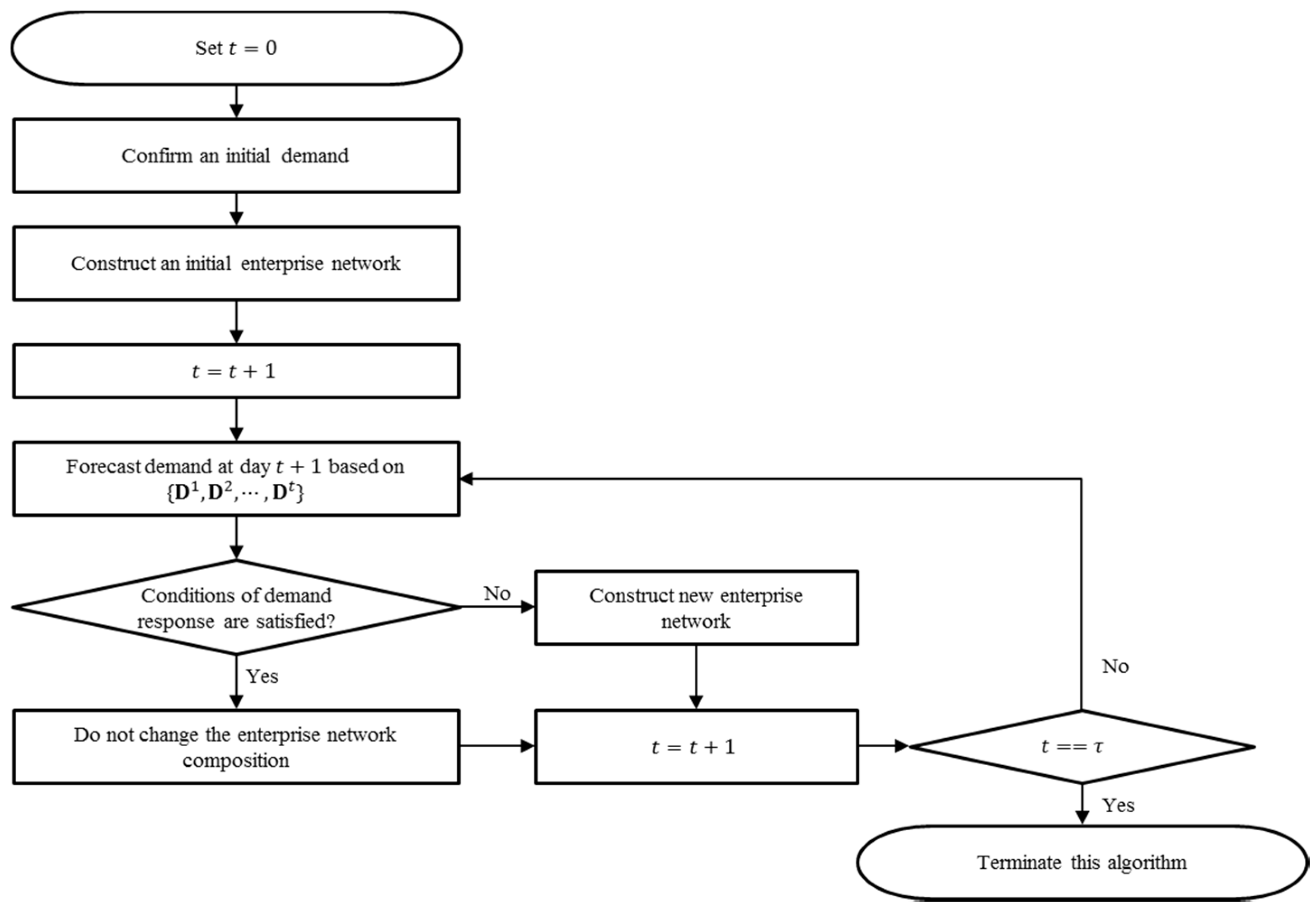
Enterprises which participate in CM should be considered as an inventory unit for scheduling or resource allocation since their resources ensure the circulation of whole manufacturing activities by cooperating with each other in the production network. It is very important, therefore, to compose an enterprise network that handles the requirements from customers (i.e., demands) with minimal costs, and this problem is called the enterprise network composition problem in CM. It is a non-trivial problem since trade-offs exist between costs (e.g. contract cost and opportunity cost of production), and also probabilistic constraints such as forecasted demand and, therefore, it is almost impossible to find the optimal network analytically. This paper proposes a dynamic enterprise network composition algorithm (DENCA) based on a GA to solve the problem dynamically. In other words, DENCA constructs the initial enterprise network and changes the network as demand is changed.
The rest of this paper is organized as follows: Section 2 describes a research problem called the enterprise network composition problem and introduces assumptions and notations used throughout this paper; Section 3 proposes an algorithm to solve the problem, and each step of the algorithm is explained in detail; 
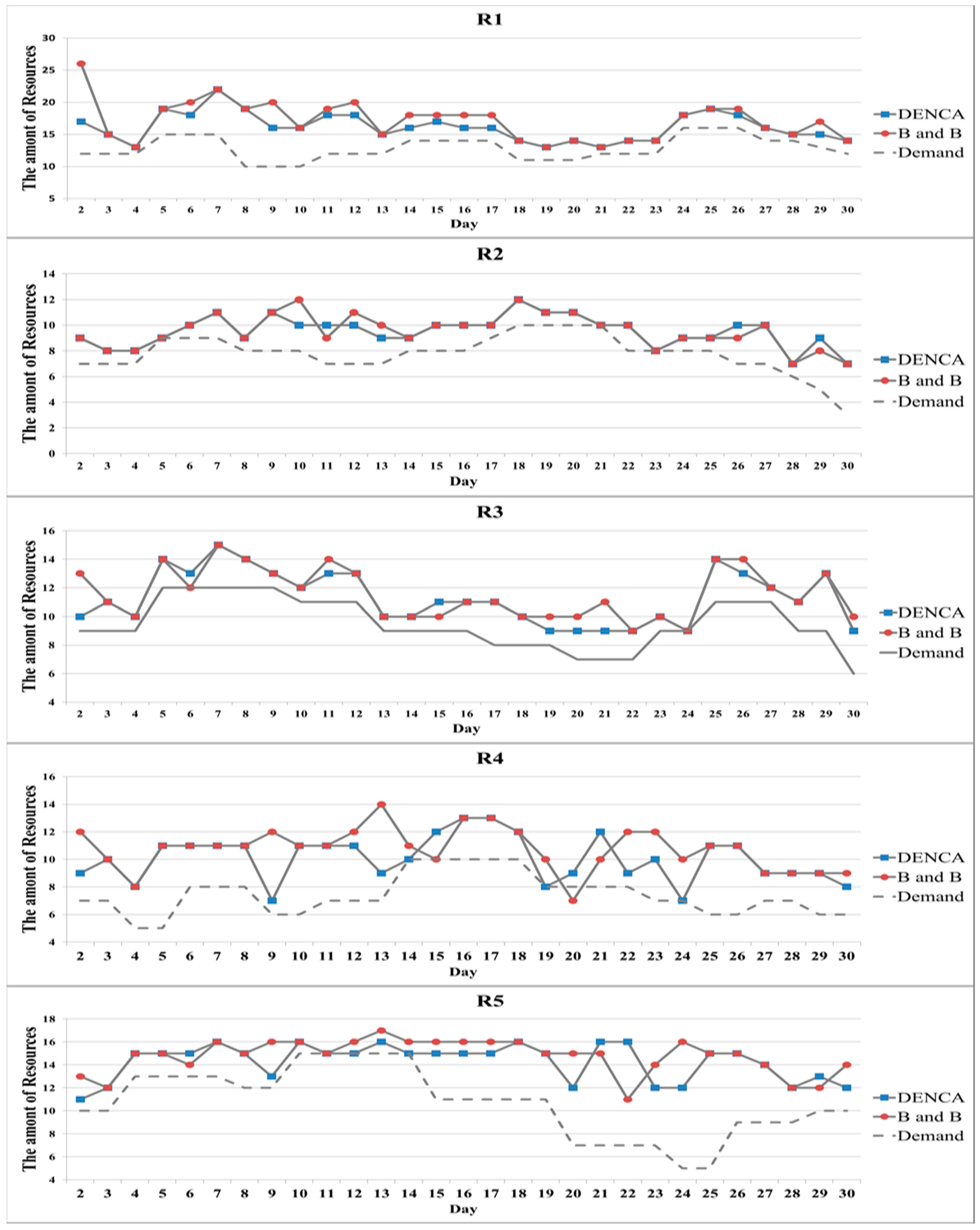
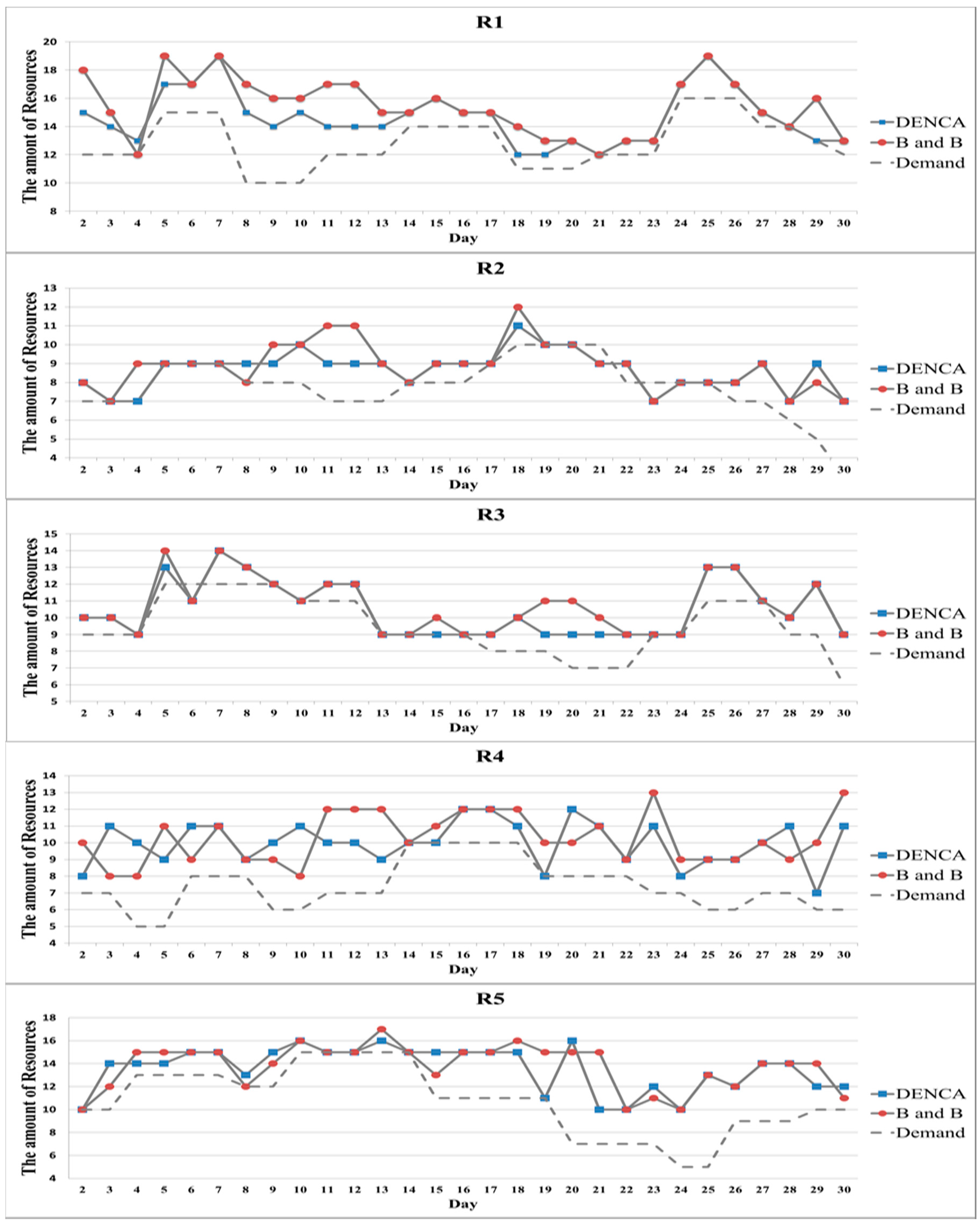
Section 4 provides a numerical simulation to illustrate the suggested algorithm; and Section 5 concludes the paper.

2. Enterprise Network Composition Problem

2.1. Description

Since one of the typical characteristics of CM is the pay-per-use of manufacturing resources on demand [5], the cost structures of existing manufacturing models and those of CM are completely different. For example, the task of inventory management for existing manufacturing models is to maintain stock of products or resources [25], while the task for CM is to sustain an appropriate enterprise network to handle various customer requests and minimize the composition cost. Note that the CM task mentioned above is the responsibility of a CM manager, not a manager of an enterprise belonging to CM. Therefore, traditional inventory costs, such as order cost and depreciation cost, are not involved, but enterprise management costs, such as contracts, service invocation, and aggregation, occur in CM [26].
It is difficult to compose a proper enterprise network so that the network can respond to the demands with minimal cost because of several practical reasons: (1) probabilistic constraints; (2) various expenses; and (3) dynamically-changing customer requests (a real-time algorithm is needed). Furthermore, the initially-composed network (initial network) could change as demands fluctuate. That is, the network may not meet later demands or need additional expenses although the network was well composed at first. Expenses in the enterprise network are incurred in various aspects: a participation contract cost occurs when an enterprise contracts with CM to newly participate in CM, while a contract cancellation cost occurs when an enterprise cancels the contract to leave the system. Network management cost is a fixed cost, which includes an activating search engine fee, maintenance cost of the user interface, and portal website. Cloud service invocation and service aggregation costs are costs to realize manufacturing services of each enterprise in CM and to aggregate different manufacturing services (e.g., design service, logistics service), respectively. These costs are directly proportional to the amount of resources enterprises reserve [27]. Finally, the opportunity cost of production occurs when there are customer requests and the CM cannot deal with due to the lack of resources. Namely, the opportunity cost of production occurs when the CM misses a chance to make profit by handling the requests. Among the costs, some are directly proportional to the amount of resources an enterprise network has (currently retains). The enterprise management cost, including resource virtualization cost, is the typical example.
It can be intuitively known that there are trade-offs among the costs. For example, if CM contracts many enterprises to participate in CM, then the opportunity cost of production may decrease, while the enterprise management cost will increase. Another example is a trade-off between the participation contract (or contract cancellation) cost and the opportunity cost of production. If a CM manager decides to frequently change the network according to forecasted demands for a flexible operation, then the opportunity cost of production would be minimized, but contract costs and contract cancellation costs would increase. Hence, it is essential to consider these trade-offs for composing a network of enterprises. We call this the enterprise network composition problem throughout the paper.
In Figure 3, a dotted rectangle indicates the scope of the paper. We develop an algorithm to compose the enterprise network, which helps CM to match services by ensuring proper levels of demand response. It does not include resource allocation, service matching, and scheduling.

2.2. Assumptions and Notations

Initial demand (i.e., demand on day 1) is assumed to be given in advance, while subsequent demands after day 1 must be forecasted. The demands for any manufacturing services are decomposed of each type of required resource. For instance, a demand may be composed of one design resource, two production resources, and one logistics resource. The resources a network retains, but not uses, are always available whenever relevant requests arrive at the MC. If there are not sufficient resources for completing the requests, then the requests will be lost. In addition, contracts regarding enterprise participation in, or withdrawal from, the MC will take effect after a day. In other words, if a company contracts a MC to participate in, or cancel, the contracts to leave the system, then the company will join or leave the system on the next day. Finally, some events to make resources unavailable, such as unexpected maintenance, are not introduced in this paper, but we can introduce the unexpected maintenance into the model by letting the available resources be zeroes during the maintenance period.
Notations used throughout the paper are presented in the following Table 1.

3. Dynamic Enterprise Network Composition Algorithm

Figure 4 is a flow chart of the dynamic enterprise network composition algorithm (DENCA) suggested in this research. Initially, the operation day (indicated by t ) is set to 0 and initial demand D 1 is given. Then the CM manager constructs an initial enterprise network that can fully respond to the initial demand with minimal cost. With the network P E t at day t which handles the current demand, the manager forecasts demand at day ( t + 1 ) based on D 1   , D 2 , …, D t and decides whether the current network P E t can handle the predicted demand D ^ t + 1 or not. In addition, it should take into consideration that a large portion of resources retained in the current MC may not be used and wasted (i.e., utilization of MC is low) because many unnecessary enterprises are participating in the present MC. Unless the current network is expected to be satisfied with the conditions (the enterprise network is able to handle future demand properly, and resource waste problems should not occur), the manager should construct a new enterprise network and these steps repeat for the entire operating time span.
A detailed explanation of the flowchart in Figure 4 will be provided from Section 3.1, Section 3.2, Section 3.3 and Section 3.4. More concretely, Section 3.1 and Section 3.2 describe how to construct an initial enterprise network and to forecast demand at day t + 1 based on { D 1 , D 2 ,   ,   D t } , respectively. In Section 3.3, we explain how one can check if constraints of the demand response are satisfied and, finally, Section 3.4 explains the way to construct a new enterprise network when the conditions of the demand response are not satisfied utilizing a genetic algorithm.

3.1. Initial Enterprise Network Composition

The initial enterprise network should cover the initial demands with minimal cost. The formulation for the initial enterprise network composition problem is presented in Equations (1) and (2). The objective function in Equation (1) is to minimize the cost when the initial network is P E 1 , which consists of the CM internal management cost ( C IN ( P E 1 ) ) and the participation contract cost ( i = 1 n ( I i 1 × C co ( E i ) ) ). Note that the contract cancellation and opportunity cost of production are not included in the objective function in Equation (1) because the initial network is constructed to handle the initial demand without any loss. Constraints in Equation (2) imply that the number of resources R j   ( j = 1 , 2 , , m ) the initial network possesses must be larger than, or equal to, the initial demand of R j .
Min   Z = C IN ( P E 1 ) +   i = 1 n ( I i 1   × C co ( E i ) )
subject to:
i = 1 n I i 1 × λ j ( E i ) D j 1 ,   for   all   j = 1 ,   2 ,   ,   m ,   I i 1 { 0 ,   1 }
The internal management cost of the MC in Equation (1) is calculated as follows:
C IN ( P E t ) =   E j P E t { C SI ( E j ) + C SA ( E j ) }
Cloud service invocation, cloud service aggregation, and participation contraction costs of E i are calculated in Equations (4)–(6), respectively:
C SI ( E i ) =   j = 1 m ( λ j ( E i ) ×   C SI ,   R j )
C SA ( E i ) =   j = 1 m ( λ j ( E i ) ×   C SA ,   R j )
C CO ( E i ) =   j = 1 m ( λ j ( E i ) ×   C CO ,   R j )  
where C SI ,   R j , C SA ,   R j , and C CO , R j denote the unit cost of cloud service invocation, cloud service aggregation, and participation contraction for R j . C SI , R j is interpreted as the cost to aggregate one additional resource R j . C SA ,   R j and C CO ,   R j can be interpreted similarly. Equations (4)–(6) indicate that these costs are directly proportional to the amount and kind of resource E i has. Thus, the objective function in Equation (1) can be re-written as follows:
Min   Z =   E j P E 1 { j = 1 m ( λ j ( E i ) ×   C SA ,   R j ) + j = 1 m ( λ j ( E i ) ×   C SI ,   R j ) } +   i = 1 n ( I i 1   × j = 1 m ( λ j ( E i ) ×   C CO ,   R j ) )
The initial enterprise network composition problem can be solved by integer linear programming (ILP), whose decision variable I i 1 ( i = 1 ,   2 ,   ,   n ) indicates whether E i participates in CM ( I i 1 = 1 ) or not ( I i 1 = 0 ) at t = 1 .

3.2. Resource Demand Forecasting

Time-series analysis methods have been employed to forecast demand of enterprise resources, including cloud computing resources, in many studies. For example, Zhang et al. [28] employed auto-regressive (AR) functions to forecast demand for CPU and memory in a cloud computing environment. Let T ( ) be a time-series model for forecasting demand D j t + 1   ( j = 1 ,   2 ,   ,   m ) at t + 1 . Then:
D j t + 1 = T ( D j 1 ,   ,   D j t ) + ε j = D ^ j t + 1 + ε j  
where the forecasting error ε j is assumed to follow a Gaussian distribution with mean 0 and variance σ j 2 , which is time-independent. Therefore, D j t + 1 is a random variable which also follows a Gaussian distribution with mean D ^ j t + 1 and variance σ j 2 . Then we have:
D t + 1 = ( T ( D 1 ) ,   ,   T ( D m ) ) T + ε
where T ( D j ) = T ( D j 1 ,   ,   D j t ) for j = 1 , 2 , ,   m and ε = ( ε 1 ,   ε 2 ,   ,   ε m ) T .
Note that the D j t denotes the amount of resource j required at day t . For instance, if a task which requires three resource j for two days is arrived at day t , and there is no other task in CM but the task, then the D j t and D j t + 1 will be 3.

3.3. Conditions of Demand Response

The condition in Equation (10) helps us determine whether the current network should be reconstructed or not in order to handle the current demands properly and not to waste resources:
P ( i = 1 n ( I i t × λ j ( E i ) ) < D ^ j t + 1 ) < α   for   j = 1 ,   2 ,   ,   m
Inequality in Equation (10) indicates the probability that the capacity of R j   ( j = 1 , 2 , , m ) in the current enterprise network is not sufficient for the demand of the next day and should be smaller than user parameter α , the threshold of the risk that demand will not be met. Notice that the value of α should be small if the loss unit cost is high. By means of a standard normal distribution, the probability can easily be calculated. Another set of inequalities to be considered is the following:
P ( E i P E t { PE j t } ( I i t × λ j ( E i ) ) < D ^ j t + 1 ) < α ,        for   j = 1 , 2 ,   ,   m , k = 1 ,   2 ,   , | P E t |
Inequality in Equation (11) expresses the probability that an enterprise network could handle the demand properly, even if an arbitrary enterprise currently participating in the MC leaves. This must be larger than 1 α .

3.4. Enterprise Network Recomposition

If the conditions introduced in Section 3.3 are not satisfied, then the enterprise network should be newly composed. We call this recomposition of the network. Recomposition is noticeably different from the initial network composition because the demand loss probability must be considered, as well as both contract cancellation cost and opportunity cost of production for the network.
The recomposition procedure can be done by solving the following:
Min   Z = i = 1 n ( I i t + 1   × ( C SA ( E i ) + C SI ( E i ) ) + E i P E t ( I i t + 1 × C CO ( E i ) ) + E i P E t ( ( 1 I i t + 1 ) × C CW ( E i ) ) +   C LO ( P E t + 1 )  
subject to:
P ( i = 1 n ( I i t + 1 × λ j ( E i ) ) < D ^ j t + 1 ) < α ,      for   j = 1 ,   2 ,   3 ,   ,   m .
The first term i = 1 n ( I i t + 1   × ( C SA ( E i ) + C SI ( E i ) ) in Equation (12) denotes total cloud service aggregation and invocation costs incurred by enterprises participating in CM. The second term E i P E t ( I i t + 1 × C CO ( E i ) ) is the total contract cost incurred by newly-participating enterprises. The third term E i P E t ( ( 1 I i t + 1 ) × C CW ( E i ) ) is the total contract cancellation cost incurred by newly-leaving enterprises, where C CW ( E i ) is calculated as following:
C CW ( E i ) =   j = 1 m ( λ j ( E i ) ×   C CW ,   R j )  
Finally, C LO ( P E t + 1 ) denotes the opportunity cost of production when the enterprise network is P E t + 1 , which is given by:
C LO ( P E t ) = j = 1 m ( g ( E i P E t λ j ( E i ) ,    D j t ) × C LO ,   R j )
where g ( E i P E t λ j ( E i ) ,    D j t ) is the amount of loss for R j .
g ( E i PE t λ j ( E i ) , D j t ) =   { D j t E i PE t λ j ( E i ) , if   D j t > E i PE t λ j ( E i ) ,   0 , otherwise .
In contrast to the initial network construction, ILP cannot be adopted to recompose the network because of probabilistic constraints. Instead, a metaheuristic algorithm must be used to solve this efficiently and GA is employed in this paper. We represent the structure of chromosomes as a binary string of n bits where each bit denotes whether a corresponding enterprise participates in the system or not.

4. Numerical Example

This section provides a numerical example to illustrate and compare efficiencies of the suggested algorithm in this study and the branch-and-bound (B and B) algorithm. In Section 4.1, we generate a set of simulated data including information of enterprises and estimated demands for an experiment. In Section 4.2, we apply DENCA to this simulated dataset.

4.1. Data

We assume that there are 15 enterprises ( E 1 , , E 15 ) and five resources ( R 1 , , R 5 ) . The amount of resources each enterprise possesses are presented in Table 2. Each resource can be a manufacturing resource (e.g., robot arm, 3D printer), a logistic resource (e.g., truck, airplane), etc. As shown, each enterprise has four or five kinds of resources and, therefore, simple inventory models cannot be applied to this problem.
CM is assumed to operate for 30 days ( τ = 30 ), and the actual and forecasted demands of each resource are shown in Table 3 ((a) and (b)), respectively. Forecasted demands are obtained by adding random noise ε j   ( j = 1 , , 5 ) to actual demands of each resource for 30 days, where ε 1 ,   ε 2 ,   ε 3   ~   N ( 0 ,   1 2 ) and ε 4 ,   ε 5   ~   N ( 0 ,   0.5 2 ) .

4.2. Results

Using the formulation in Section 3.1, we compose the initial network by searching all possible enterprise combinations. In other words, we attempt to find the solution satisfying every constraint and minimizing the costs in Equation (1) from ( 0 ,   0 ,   0 ,   0 ,   0 ,   0 ,   0 ,   0 ,   0 ,   0 ,   0 ,   0 ,   0 ,   0 ,   0 ) to ( 1 ,   1 ,   1 ,   1 ,   1 ,   1 ,   1 ,   1 ,   1 ,   1 ,   1 ,   1 ,   1 ,   1 ,   1 ) . The optimal initial network, its capacity for each resource, and its related cost are ( 1 , 1 , 1 , 1 , 1 , 1 , 1 , 1 , 1 , 0 , 0 , 0 , 1 , 1 , 0 ) , ( λ 1 ( P E 1 ) ,   ,   λ 5 ( P E 1 ) ) = ( 23 ,   14 ,   16 ,   13 ,   17 ) , and 18,070, respectively.
Now, for values α = 0.1 and 0.2 , we construct enterprise networks in CM from day 2–30, as explained in Section 3.4, by means of the suggested algorithm, and a B and B algorithm for comparison purpose. The B and B algorithm is employed because it is known to yield good outputs for IP problems in general. Figure 5 and Figure 6 illustrate the amount of each resource of the enterprise networks constructed by means of the DENCA and B and B algorithms when α = 0.1   and 0.2 , respectively. These figures also include the actual demands for 29 days (from day 2 to day 30).
As shown in these figures, the enterprise networks constructed through both the DENCA and B and B algorithms can handle the demand without any loss for each resource. In other words, the amounts of resources that the enterprise networks have are higher than the amounts of required resources (i.e., demands) for the entire 30 days. The difference between the enterprise networks derived from the DENCA and B and B algorithms is that the former prepares more resources than the latter, which might cause resource waste (unnecessary expense). Readers see that most red circle points (derived from B and B) are located above the blue square points (obtained by DENCA) and dotted lines (actual demand) in the figures.
Table 6 demonstrates the overall network composition costs calculated by the DENCA and B and B algorithms and it supports that the overall network composition costs by means of DENCA is equal to, or less than, the overall network composition costs by means of the B and B algorithm for all days.

5. Conclusions

CM can help enterprises (especially SMEs) perform large-scale manufacturing jobs by collaborating with other enterprises, but several critical issues for practical operations remain to be resolved. In this study, we suggested an algorithm based on GA for the enterprise network selection problem, which is one of these problems. This algorithm includes composing an initial enterprise network, forecasting demand, and recomposing the network according to demand forecasts. A numerical example was provided to show that the network constructed by means of the suggested algorithm not only handles the demands better, but also incurs a smaller cost (note that no significant difference was observed between network capacities and actual demands) than the B and B algorithm. In addition, the suggested algorithm is cheaper than the B and B algorithm in terms of computational time.
Since this paper is based on the some assumptions (e.g., the initial demand is given in advance, the forecasting error term follows a Gaussian distribution), this paper may not completely describe and reflect CM situations well. Hence, these assumptions should be eased in our future research. For example, we did not consider the situation that enterprises have trouble in collaborating with each other because of an assumption that enterprises are located near each other. Thus, we will consider collaboration potentials among enterprises based on enterprises’ locations, quality evaluations, etc., in future research.

Acknowledgments

This work was supported by NRF (National Research Foundation of Korea) Grant funded by the Korean Government (NRF-2016-Fostering Core Leaders of the Future Basic Science Program/Global Ph.D. Fellowship Program).

Author Contributions

Gilseung Ahn, You-Jin Park, and Sun Hur conceived and designed the research; Gilseung Ahn conducted the research and drafted the manuscript. Sun Hur revised the manuscript and You-Jin Park supervised the overall work. All authors read and approved the final manuscript.

Conflicts of Interest

The authors declare no conflict of interest.

References

  1. Wang, Z.; Zhang, M.; Sun, H.; Zhu, G. Effects of standardization and innovation on mass customization: An empirical investigation. Technovation 2016, 48, 79–86. [Google Scholar] [CrossRef]
  2. Ferguson, S.M.; Olewnik, A.T.; Cormier, P. A review of mass customization across marketing, engineering and distribution domains toward development of a process framework. Res. Eng. Des. 2014, 25, 11–30. [Google Scholar] [CrossRef]
  3. Li, B.; Zhang, L.; Wang, S.L.; Tao, F.; Cao, J.W.; Jiang, X.D.; Chai, X.D. Cloud manufacturing: A new service-oriented networked manufacturing model. Comput. Integr. Manuf. Syst. 2010, 16, 1–7. [Google Scholar]
  4. Mell, P.; Grance, T. The NIST Definition of Cloud Computing; National Institute of Standards and Technology: Gaithersburg, MD, USA, 2011. [Google Scholar]
  5. Wu, D.; Greer, M.J.; Rosen, D.W.; Schaefer, D. Cloud manufacturing: drivers, current status, and future trends. In Proceedings of the ASME 2013 International Manufacturing Science and Engineering Conference Collocated with the 41st North American Manufacturing Research Conference, Madison, WI, USA, 10–14 June 2013.
  6. Zhang, L.; Luo, Y.; Fan, W.; Tao, F.; Ren, L. Analysis of cloud manufacturing and related advanced manufacturing models. Comput. Integr. Manuf. Syst. 2011, 17, 458–468. [Google Scholar]
  7. Xu, J.; Chen, P. Study on Objects Ordering for Manufacturing Cloud Platform. In Proceedings of the International Conference on Information Engineering and Applications, London, UK, 26–28 October 2012; pp. 431–437.
  8. Huang, B.; Li, C.; Yin, C.; Zhao, X. Cloud manufacturing service platform for small-and medium-sized enterprises. Int. J. Adv. Manuf. Technol. 2013, 65, 1261–1272. [Google Scholar] [CrossRef]
  9. Xu, X. From cloud computing to cloud manufacturing. Robot. Comput.-Integr. Manuf. 2012, 28, 75–86. [Google Scholar] [CrossRef]
  10. Wu, D.; Rosen, D.W.; Wang, L.; Schaefer, D. Cloud-Based Manufacturing: Old Wine in New Bottles? Procedia CIRP 2014, 17, 94–99. [Google Scholar] [CrossRef] [Green Version]
  11. Tao, F.; Zhang, L.; Venkatesh, V.C.; Luo, Y.; Cheng, Y. Cloud manufacturing: A computing and service-oriented manufacturing model. J. Eng. Manuf. 2011. [Google Scholar] [CrossRef]
  12. Laili, Y.; Tao, F.; Zhang, L.; Cheng, Y.; Luo, Y.; Sarker, B.R. A Ranking Chaos Algorithm for dual scheduling of cloud service and computing resource in private cloud. Comput. Ind. 2013, 64, 448–463. [Google Scholar] [CrossRef]
  13. Cao, Y.; Wang, S.; Kang, L.; Gao, Y. A TQCS-based service selection and scheduling strategy in cloud manufacturing. Int. J. Adv. Manuf. Technol. 2016, 82, 235–251. [Google Scholar] [CrossRef]
  14. Mai, J.; Zhang, L.; Tao, F.; Ren, L. Customized production based on distributed 3D printing services in cloud manufacturing. Int. J. Adv. Manuf. Technol. 2016, 84, 71–83. [Google Scholar] [CrossRef]
  15. Li, W.; Zhu, C.; Yang, L.T.; Shu, L.; Ngai, E.C.H.; Ma, Y. Subtask Scheduling for Distributed Robots in Cloud Manufacturing. IEEE Syst. J. 2015, 99, 1–10. [Google Scholar] [CrossRef]
  16. Wei, X.; Liu, H. A cloud manufacturing resource allocation model based on ant colony optimization algorithm. Int. J. Grid Distrib. Comput. 2015, 8, 55–66. [Google Scholar] [CrossRef]
  17. Tsai, J.T.; Fang, J.C.; Chou, J.H. Optimized task scheduling and resource allocation on cloud computing environment using improved differential evolution algorithm. Comput. Oper. Res. 2013, 40, 3045–3055. [Google Scholar] [CrossRef]
  18. Ren, L.; Cui, J.; Wei, Y.; LaiLi, Y.; Zhang, L. Research on the impact of service provider cooperative relationship on cloud manufacturing platform. Int. J. Adv. Manuf. Technol. 2016, 86, 2279–2290. [Google Scholar] [CrossRef]
  19. Argoneto, P.; Renna, P. Supporting capacity sharing in the cloud manufacturing environment based on game theory and fuzzy logic. Enterp. Inf. Syst. 2016, 10, 193–210. [Google Scholar] [CrossRef]
  20. Renna, P. Decision model to support the SMEs’ decision to participate or leave a collaborative network. Int. J. Prod. Res. 2013, 51, 1973–1983. [Google Scholar] [CrossRef]
  21. Rahman, H.F.; Sarker, R.; Essam, D. A real-time order acceptance and scheduling approach for permutation flow shop problems. Eur. J. Oper. Res. 2015, 247, 488–503. [Google Scholar] [CrossRef]
  22. Lei, H.; Wang, R.; Zhang, T.; Liu, Y.; Zha, Y. A multi-objective co-evolutionary algorithm for energy-efficient scheduling on a green data center. Comput. Oper. Res. 2016, 75, 103–117. [Google Scholar] [CrossRef]
  23. Ma, J.; Li, W.; Fu, T.; Yan, L.; Hu, G. A Novel Dynamic Task Scheduling Algorithm Based on Improved Genetic Algorithm in Cloud Computing. In Wireless Communications, Networking and Applications; Springer: New Delhi, Germany, 2016; pp. 829–835. [Google Scholar]
  24. Sethanan, K.; Chamnanlor, C.; Chien, C.; Gen, M. Hybrid Genetic Algorithms for Solving Reentrant Flow-Shop Scheduling with Time Windows. Ind. Eng. Manag. Syst. 2013, 12, 306–316. [Google Scholar]
  25. Basu, R.; Wright, J. Inventory management. In Total Supply Chain Management; Routledge: London, UK, 2010; pp. 96–108. [Google Scholar]
  26. Chen, F.; Dou, R.; Li, M.; Wu, H. A flexible QoS-aware Web service composition method by multi-objective optimization in cloud manufacturing. Comput. Ind. Eng. 2016, 99, 423–431. [Google Scholar] [CrossRef]
  27. Cheng, Y.; Zhao, D.; Hu, A.R.; Luo, Y.L.; Tao, F.; Zhang, L. Multi-view models for cost constitution of cloud service in cloud manufacturing system. In Advances in Computer Science and Education Applications, Proceedings of the International Conference, CSE 2011, Qingdao, China, 9–10 July 2011; Springer: Berlin/Heidelberg, Germany, 2011; pp. 225–233. [Google Scholar]
  28. Zhang, Q.; Zhani, M.F.; Zhang, S.; Zhu, Q.; Boutaba, R.; Hellerstein, J.L. Dynamic energy-aware capacity provisioning for cloud computing environments. In Proceedings of the 9th international conference on Autonomic computing, San Jose, CA, USA, 16–20 September 2012; pp. 145–154.
Figure 1. Operation process of cloud manufacturing.
Sustainability 08 01239 g001
Figure 2. The whole life cycle process of CM.
Sustainability 08 01239 g002
Figure 3. Operation process of cloud manufacturing.
Sustainability 08 01239 g003
Figure 4. Flowchart of the proposed algorithm.
Sustainability 08 01239 g004
Figure 5. The amount of each resource the constructed networks own when α = 0.1 and actual demand.
Sustainability 08 01239 g005
Figure 6. The amount of each resource the constructed networks own when α = 0.2 and actual demand.
Sustainability 08 01239 g006
Table 1. Notations.
Table 1. Notations.
NotationDefinition
E i Enterprise i , i = 1 , 2 , , n
I i t Indicator variable which represents whether the enterprise i joins the network at day t or not, that is, I i t = 0 or 1
P E t Set of participating enterprises in an enterprise network at day t
PE i t Participating enterprise i in an enterprise network at day t
R j Resource j    ( j = 1 , , m )
D j t Demand of R j at day t
D t Vector of demands at day t , ( D 1 t ,   D 2 t ,    , D m t )
D ^ j t Forecasted demand of R j at day t
λ j ( E i ) E i ’s capacity of resource R j
λ j ( P E t ) Current enterprise network’s capacity of resource R j
C IN ( P E t ) Internal management cost of MC of P E t
C SI ( E i ) Cloud service invocation cost of E i
C SA ( E i ) Cloud service aggregation cost of E i
C CO ( E i ) Participation contract cost of E i
C CW ( E i ) Contract cancellation cost of E i
C LO ( P E t ) Opportunity cost of production occurring when P E t do not respond demand properly at day t
C SI , R j Unit cost of cloud service invocation for R j
C SA , R j Unit cost of cloud service aggregation for R j
C CO , R j Unit cost of participation contract for R j
C CW , R j Unit cost of contract cancellation for R j
C LO , R j Unit opportunity cost of production for R j
α Significance level of the risk that demand is unmet (user-defined parameter)
τ Number of operation days of MC (user-defined parameter)
Table 2. Amount of resources each enterprise reserves.
R 1 R 2 R 3 R 4 R 5
E 1 20121
E 2 41201
E 3 31032
E 4 02105
E 5 50210
E 6 11220
E 7 32101
E 8 01134
E 9 21310
E 10 40122
E 11 13102
E 12 21011
E 13 04113
E 14 31200
E 15 05121
Table 3. The amount of resources each enterprise reserves.
(a) Actual Demands(b) Forecasted Demands
t D 1 t D 2 t D 3 t D 4 t D 5 t D ^ 1 t D ^ 2 t D ^ 3 t D ^ 4 t D ^ 5 t
11279710-----
21279710127879
312797101369710
412795131168513
51591251315612513
61591281316810713
71591281313813712
8108128129712711
9108126128811512
101081161510810515
111271171512611714
121271171511811614
1312797151368615
14148910151478914
15148910111588910
161489101114881011
171498101114881010
1811108101191071010
19111088111196710
201110787129666
211210787108787
22128787128687
23128977126876
24168975167765
2516811651771254
2616711691671158
2714711791481089
28146979135988
29135961012311610
3012366101246610
The unit costs and corresponding costs are presented in Table 4 and Table 5, respectively.
Table 4. Unit costs of each resource.
R 1 R 2 R 3 R 4 R 5
C S A , R k 2025202520
C S I , R k 2025152520
C C O , R k 5060407060
C C W , R k 3040305040
C L O , R k 6075608070
Table 5. Corresponding costs related with each enterprise.
C S A C S I C C O C C W
E 1 130125340230
E 2 16515540026
E 3 200200540360
E 4 170165460310
E 5 165155400260
E 6 135125330230
E 7 150145370240
E 8 200195550380
E 9 150135350240
E 10 190185500330
E 11 155150390260
E 12 110110290190
E 13 205200530360
E 14 125115290190
E 15 215210540370
Table 6. Network composition costs by means of the DENCA and B and B algorithms.
α = 0.1 α = 0.2
DayDENCAB and BDENCAB and B
212,96013,06512,93012,960
313,31513,31513,29013,300
413,55013,55013,53513,545
513,64013,64013,61513,640
613,63513,65013,60513,605
713,69513,69513,64013,640
813,64013,64013,59513,605
913,62513,66513,58013,610
1013,61013,63013,59513,605
1113,63513,64013,58013,630
1213,63513,66513,58013,630
1313,58013,59013,56513,575
1413,59013,61013,56513,565
1513,61513,62013,58513,590
1613,60513,62513,57513,575
1713,60513,62513,57513,575
1813,60013,60013,57013,600
1913,57513,58013,55513,575
2013,58513,59013,56513,575
2113,56513,57513,54513,550
2213,57513,57513,55513,555
2313,56013,56013,53513,535
2413,60513,60513,58513,585
2513,64013,64013,62513,625
2613,63513,64013,60513,605
2713,61013,61013,58513,585
2813,56513,56513,55013,550
2913,59513,60513,57013,590
3013,54513,55013,53513,535

