Environmental Efficiency of Chinese Open-Field Grape Production: An Evaluation Using Data Envelopment Analysis and Spatial Autocorrelation

Abstract

Grape production is associated with some negative environmental externalities. However, they are not considered in the traditional data envelopment analysis (DEA) efficiency assessment models and the research literature. Hence, the assessment results cannot correctly reflect the technical efficiency level of open-field grape production. We measured the environmental efficiency of China’s open-field grape production under the constraint of carbon emissions using the slacks-based measure (SBM) model, including the undesirable outputs. In addition, spatial relations of environmental efficiency in different open-field grape production areas in China were evaluated by adopting spatial econometric methods. The results indicate that the average environmental efficiency score of grape production in China is at a low level of 0.651. Overall, the average environmental efficiencies in southern, southwest, and northeast regions are lower than the average levels, which implies the imbalance in economic outputs, resource consumption, and environmental efficiency in open-field grape cultivation. Moreover, the spatial autocorrelation results show that the environmental efficiency of grape production has obvious continuity in neighboring regions and spatial correlation.

1. Introduction

The environmental problems caused by greenhouse gas emissions have brought significant adverse effects to human health and economic development, and have gradually become the major issues of concern to countries around the world [1]. The Intergovernmental Panel on Climate Change (IPCC) has stressed that agriculture has become the second largest source of greenhouse gas emissions, and its emissions have been as high as the global anthropogenic emissions of 13.5% in the fourth assessment report [2]. Chinese agriculture is changing from extensive agriculture to a more intensive type and greater importance is being stressed on ecological and environmentally friendly production patterns. However, a large amount of fertilizer and pesticides have been invested in the process of agricultural production, driven by economic benefits, which has inevitably led to serious agricultural environmental problems that have badly hindered the process of agricultural modernization in China. Therefore, it is the unwaveringly future trend to achieve sustainable and harmonious development in the agricultural economy and ecological environmental protection in modern agriculture in China.

Currently, viticulture has become an important part of China’s agriculture. According to the statistics of the Chinese Agricultural Research System [3], the total area for Chinese open-field grape cultivation exceeds 500,000 hectares, and amounts for about 80% of the total viticulture. However, the pursuit of high economic benefits simply could not be in accordance with the concept of sustainable development, so the ecological benefits of open-field grape cultivation and sustainable development gradually attracted universal attention. Studies have shown that open-field grape cultivation will bring high carbon emissions and other environmental hazards, so it faces the problem of a threat to the sustainable development of production systems and significant environmental pressure [4,5,6]. Hence, it is necessary to accurately measure the environmental efficiency of open-field grape production in various regions of China, so as to adjust resource consumption, achieving energy-saving and the reduction of emissions and improving the environmental performance in viticulture.

Many theories and methods for environmental efficiency assessment are currently available, such as life-cycle analysis [7,8,9,10], the ecological footprint method [11,12,13], material flow analyses [14,15], the multiple-criteria decision-making method[16], the clustering method [17], production frontal analysis, which mainly includes stochastic frontier analysis (SFA) [18,19,20,21], and data envelopment analysis (DEA) [22,23,24]. Among these methods, the DEA method has been widely used to evaluate environmental efficiency [25,26,27].

As far as environmental efficiency is concerned, various studies based on experimental research show that the spatial factor may play a key role in environmental efficiency differences [28]. It is necessary to research the spatial characteristics of the environmental efficiency of grape production since viticulture depends highly on local endowments, such as the climate, land, and other natural resources and socioeconomic factors. There are also several published studies on spatial characteristics of environmental efficiency in various parts of the world. Camarero [29] applied variation coefficients to test for convergence of the spatial discrepancy in environmental performance. Marconi [30] performed a Moran’s statistics analysis and the local indicators of spatial association (LISA) analysis to test agri-environmental efficiency for local spatial autocorrelations. Costantini [31] adopted spatial econometrics to analyze the agglomerative effect and the environmental performance of neighboring regions in Italy. Adetutu [32] explored environmental efficiency in Europe by a multistage spatial analysis, and found that a country’s total factor productivity (TFP) growth must fall to reduce its nitrogen and sulfur emissions. Shen [33] measured the cluster of regional environmental efficiency of the Chinese industry and its overflowing effect. Zhao [34] used the spatial econometric model to evaluate the spatial distribution characteristics of the environmental efficiency of the Chinese industry.

As stated previously, it can be found that although the DEA method is widely used in environmental performance evaluation, only a few extant studies on open-field grape production are available, especially for environmental efficiency research [35]. Additionally, analysis using GIS and spatial econometrics for the characteristics of the space differences in environmental efficiency is far from adequate. Accordingly, this paper aims to explore the environmental efficiency, as well as its spatial correlation, of open-field grape cultivation in China.

The structure of this paper is organized as follows: firstly, the materials and methods are presented, in the next section the environmental efficiency of open-field grape cultivation under the view of environmental protection is evaluated, and then the spatial correlation of the environmental efficiency is discussed, and, finally, the paper concludes with implications.

2. Materials and Methods

2.1.Data Collection

In this study, the open-field grape production counties were selected as the sample. The data were collected using a questionnaire that was distributed in 119 open-field grape production counties of China. The survey was conducted in 2014 with the support of the China Agricultural Research System (CARS-30), which is a nationwide research team that focuses on the grape and wine industry.

During the investigation, 745 questionnaires were distributed to the open-field grape planters. Excluding the invalid questionnaires lacking key items and including logic errors, 494 valid questionnaires distributed were eventually reclaimed from 119 counties in China, with a validity rate of 66.31%, and the margin error of the survey with the 95% degree of confidence is 3.9%.

Following the prior research [36], the counties were divided into five main production regions to research the differences between areas using spatial autocorrelation, which are the grape production regions of North China, Northeast China, South China, Southwest China, and Northwest China.

2.2. Environmental Efficiency Analysis Based on Carbon Emission Calculation in the Production System

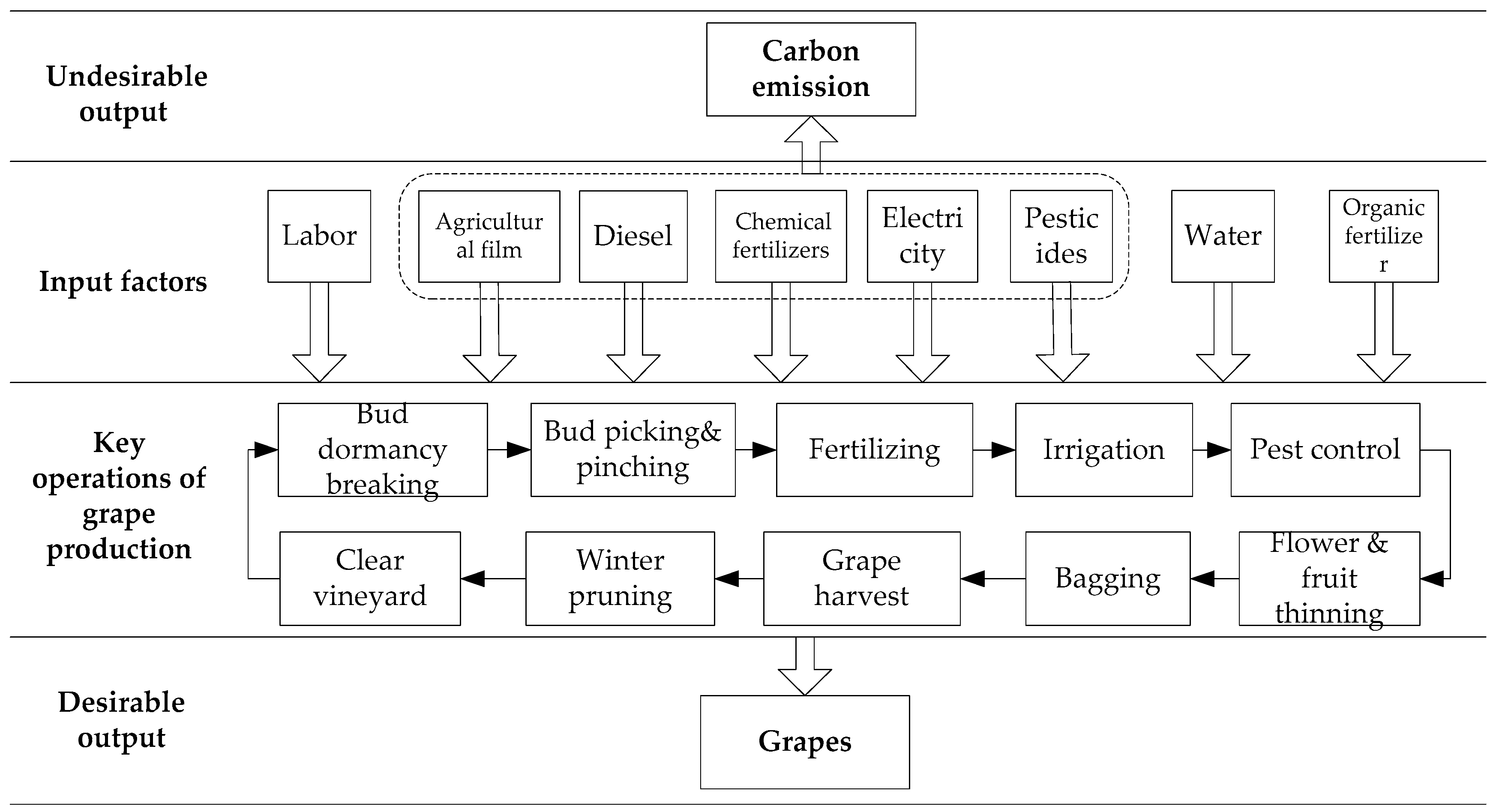
2.2.1. Open-Field Grape Production System Analysis with the Constraint of Carbon Emissions

In addition to the “desired outputs” or “good outputs” (such as grapes, etc.), the open-field grape production system may also produce some unwelcome byproducts that are called “undesirable outputs” or “bad outputs” (such as pesticide pollution, greenhouse gases emissions, etc.). The “desired outputs” and “undesirable outputs” together constitute the eco-economic system of open-field grape production, which can reflect the technical system between outputs and inputs [37]. On the one hand, open-field grape production is affected by the ecological environment; on the other hand, a series of carbon emissions in the production process of grapes, in turn, will cause an impact on the environment. Therefore, it is necessary to analyze the production process of open-field grape production under the constraint of carbon emissions, so as to ensure the accuracy and comparability of the carbon emission analysis results. The open-field grape production process, considering the carbon emissions is shown in Figure 1.

2.2.2. Carbon Emission Calculation Method

Two types of carbon emissions from open-field grape production are distinguished: direct carbon emissions and indirect carbon emissions, and their definitions are as follows:

• Direct carbon emissions include the carbon emissions from fossil energy consumption in the production process of grape, such as diesel, and so on;
• Indirect carbon emissions are carbon emissions from the production of the agricultural inputs, such as electricity, pesticides, and so on.

According to the analysis of carbon emissions in the process of open-field grape production and the relevant research [5], this paper classifies the main sources of carbon emissions in the open-field grape production process, which include the direct and indirect carbon emissions resulting from the production and use of chemical fertilizers, pesticides, agricultural film, diesel, and electricity.

Based on the above, this paper calculates the carbon emissions in the open-field grape production process. The form of function is as shown in Equation (1):

$$E={\displaystyle \sum E_i={\displaystyle \sum T_i}}\cdot {\delta }_i$$

(1)

The variable $E$ represents the total carbon emissions in the open-field grape production process, $E_i$ represents carbon emissions from various sources, $T_i$ is the amount of each carbon emission source and ${\delta }_i$ is the carbon emission coefficient of various sources. The carbon emission coefficients of different sources are shown in

Table 1. The carbon emission coefficients of different sources.

Sources	Carbon Emission Coefficient	Reference
Chemical Fertilizer	0.8956 Kg·Kg−1	West et al. [38]
Pesticides	5.10 Kg·Kg−1	Lal et al. [39]
Agricultural Film	5.18 Kg·Kg−1	Institute of Resource, Ecosystem and Environment of Agriculture of Nanjing city
Diesel	2.76 Kg·L−1	Dyer et al. [40]
Electricity	0.608 Kg·kWh−1	Pishgar-Komleh et al. [41]

.

2.3. Evaluation Model of Environmental Efficiency

Each evaluation object is regarded as a decision-making unit (DMU) in the traditional DEA model, and the DMUs constitute the evaluation group. In the analysis, each county of grape production was a DMU. Through the analysis of the variables which is obtained from the weights of input and output indicators in the DMU, the traditional DEA model can assess whether the DMU is effective [42,43]. However, the effect of “slack variables” on the efficiency is not considered in the traditional DEA model, which will result in distortion and the efficiency score will not be accurate [44].

In order to improve the traditional DEA model, the SBM model based on the undesirable output is proposed by Tone [45]. The SBM model adds slack variables into objective function so as to eliminate the effect produced by the slack variables. Assuming that there are n DMUs in the production system, and there are three vectors, which are the input vector, the desirable output vector and the undesirable output vector. The vectors can be represented as $x\in R^m$, $y^g\in R^{s1}$ and $y^b\in R^{s2}$. Then, three matrices are defined as $X$, $Y^g$, and $Y^b$, where $X=[x_1,\cdots ,x_n]\in R^{m\times n}$, $Y^g=[y_1^g,\cdots ,y_n^g]\in R^{s_1\times n}$, and $Y^b=[y_1^b,\cdots ,y_n^b]\in R^{S_2\times n}$. Additionally, $X>0$, $Y^g>0$, and $Y^b>0$. The production set can be defined as follows: $P=\left\{(x,y^g,y^b)|x\ge X\lambda ,y^g\le Y^g\lambda ,\lambda \ge 0\right\}$. Then, the SBM model based on the undesirable output can be expressed as:

$$\begin{gathered} \rho \ast =\min \frac{1-\frac{1}{m}{\displaystyle {\sum }_{i=1}^m\frac{s_i^{-}}{x_{i0}}}}{1+\frac{1}{s_1+s_2}({\displaystyle {\sum }_{r=1}^{s_1}\frac{s_r^g}{y_{r0}^g}}+{\displaystyle {\sum }_{r=1}^{s_2}\frac{s_r^b}{y_{r0}^b}})} \\ s.t.\{\begin{array}{l}{x}_0=X\lambda +s^{-}\hfill \\ y_0^g=Y^g\lambda -s^g\hfill \\ y_0^b=Y^b\lambda +s^b\hfill \\ s^{-}\ge 0,s^g\ge 0,s^b\ge 0,\lambda \ge 0\hfill \end{array} \end{gathered}$$

(2)

where $s^{-}$ is the amount of inputs that can be reduced, $s^g$ is the amount of desirable output that can be increased, and $s^b$ is the amount of undesirable output that can be reduced; $s$ denotes the slack variable of the input or output, and $\lambda$ is the vector of weight, which reflects the degree of participation of each DMU in constructing the production frontier. Additionally, $0\le \rho \ast \le 1$.

If and only if $\rho \ast =1$, that is $s^{-}=0$, $s^g=0$, and $s^b=0$, the DMU is efficient; the DMU is not completely effective when $\rho \ast =1$, but $s^{-}\ne 0$, $s^g\ne 0$, and $s^b\ne 0$, which means that the amount of output will not be changed when redundancies in inputs are reduced. The DMU is inefficient when $0\le \rho \ast <1$, thus, the inputs, desired outputs, and undesirable outputs should be improved so that the DMU can be turned into an efficient one.

In view of the characteristics of the cost inputs in open-field grape cultivation, eight input indicators were selected and regarded as the independent variables. The desirable output was grape production, and the undesirable output was set as the carbon emissions, which are shown in

Table 2. Variables of inputs and outputs.

Input/Output	Variable	Units
Input	Labor	(labor·day)/ha./year
	Agricultural film	Kg/ha./year
	Diesel	Kg/ha./year
	Chemical fertilizers	Kg/ha./year
	Electricity	kWh/ha./year
	Pesticides	Kg/ha./year
	Water	Kg/ha./year
	Organic fertilizer	Kg/ha./year
Desirable output	Grapes	Kg/ha./year
Undesirable output	Carbon emission	Kg/ha./year

. These input and output indices constituted the variables in environmental efficiency evaluation model of open-field grape cultivation.

According to Zheng [46], the results under the variable return to scale (VRS) are more reliable. Therefore, the environmental efficiency of grape production in 119 main open-field grape production counties of China was calculated based on the VRS.

2.4. Spatial Autocorrelation Model

2.4.1. The Global Autocorrelation Model of the Environmental Efficiency

Global autocorrelation is used to analyze the spatial distribution characteristics of the geographic elements or phenomena in a certain system. If the phenomenon has the same or similar tendency in the different regions, it is said that there is spatial agglomeration and positive correlations. The global Moran’s I index is often used to evaluate the global correlation [47], as shown in the Equations (3) and (4):

$$I=\frac{{\displaystyle \sum _i^n{\displaystyle \sum _{j\ne i}^n{w}_{ij}(x_i-\overline{x})(x_j-\overline{x})}}}{S^2{\displaystyle \sum _i^n{\displaystyle \sum _{j\ne i}^n{w}_{ij}}}}$$

(3)

$$S^2=\frac{1}{n}{\displaystyle \sum _{i=1}^n{(x_i-\overline{x})}^2}$$

(4)

where n is the total number of DMUs, $x_i$ is the spatial attribute value of $i$, which represents the research object, $\overline{x}$ is the average attribute’s value of all the objects, and $w_{ij}$ is the spatial weight matrix. The value of the global Moran’s I index is from −1 to 1, $I>0$ means the positive correlation exists between DMUs, and the larger the value is, the stronger the spatial correlation is; $I<0$ indicates the negative correlation; also, the DMU is random and independent when the I value is 0.

The Z test and p test are generally used to test the significant degree of spatial correlation, the Z test formula is as follows:

$$z(i)=\frac{i-E(i)}{\sqrt{\mathrm{var}(i)}}$$

(5)

In Equation (5): $E(i)$ represents the mathematical expectation; $\mathrm{var}(i)$ is the population variance. If $\left|Z\right|$ > 1.96, it shows the global Moran’s I is significant at the 5% significance level, and when $Z>0$, it shows that the DMUs have positive spatial autocorrelation; $Z<0$ indicates negative spatial autocorrelation between DMUs.

The p test is the confidence evaluation of global Moran’s I index, which is assessed several times in random tests. When p < 5%, the probability of the null hypothesis that the DMUs can be randomly distributed is very low, and it means that the DMUs have spatial autocorrelation.

2.4.2. Local Autocorrelation Analysis of the Environmental Efficiency

Local autocorrelation analysis can be used to analyze spatial correlation characteristics between a geographic region and its surroundings. To find the spatial correlation of regions, local Moran’s I index is the most widely used evaluation index [48], as is shown in Equation (6):

$$I_i(d)=Z_i{\displaystyle \sum _{j\ne i}^n{w}_{ij}{Z}_j}$$

(6)

where $Z_i$, $Z_j$ are, respectively, the deviation between the observed value and the average of $x_i$ and $x_j$; that is $Z_i=(x_i-\stackrel{\_}{x})$, $Z_j=(x_j-\stackrel{\_}{x})$. Additionally, $w_{ij}$ is the spatial weight matrix which has been standardized. $I_i>0$ indicates the autocorrelation type of High-High (H-H) or Low-Low (L-L), while, $I_i<0$ represents the type of Low-High (L-H) autocorrelation or High-Low (H-L) autocorrelation. The explanation of these four types is as follows:

High-High (H-H) type: This type of local autocorrelation means that the environmental efficiencies of the certain region itself and the surrounding areas are similar and relatively high, so the degree of spatial difference is smaller.

Low-High (L-H) type: This type indicates that the environmental efficiency of the certain region is relatively low, but environmental efficiencies of its surrounding areas are generally higher, so they are diverse in environmental efficiency, and the degree of spatial difference is relatively large.

Low-Low (L-L) type: This type means that the environmental efficiency of the certain region, itself, and its surrounding areas are similar and relatively low; there is also a small difference in spatial difference.

High-Low (H-L) type: While the environmental efficiencies of the certain region, itself, is relatively high, and environmental efficiencies of its surrounding areas are generally lower, the degree of spatial difference is larger.

3. Results

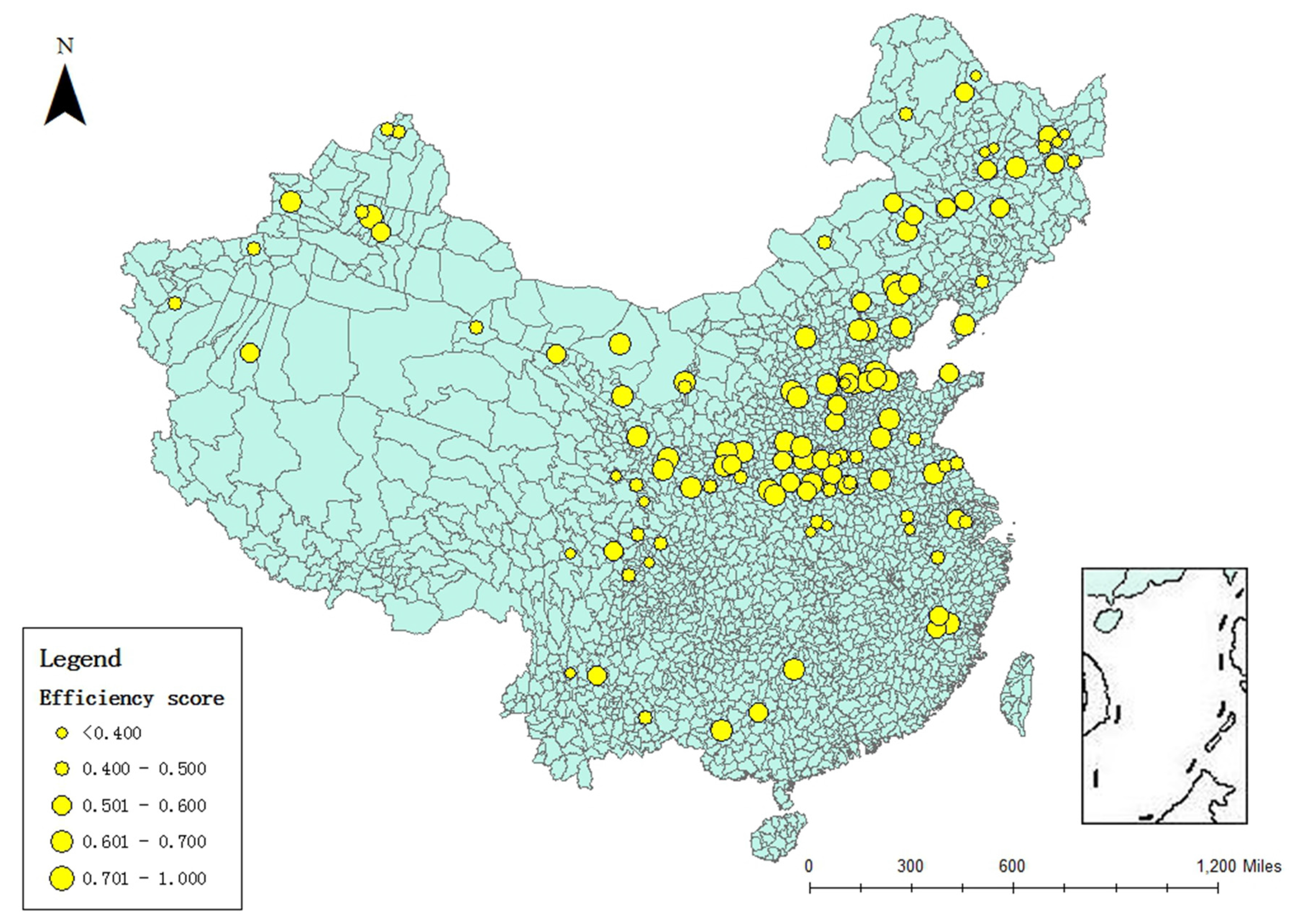
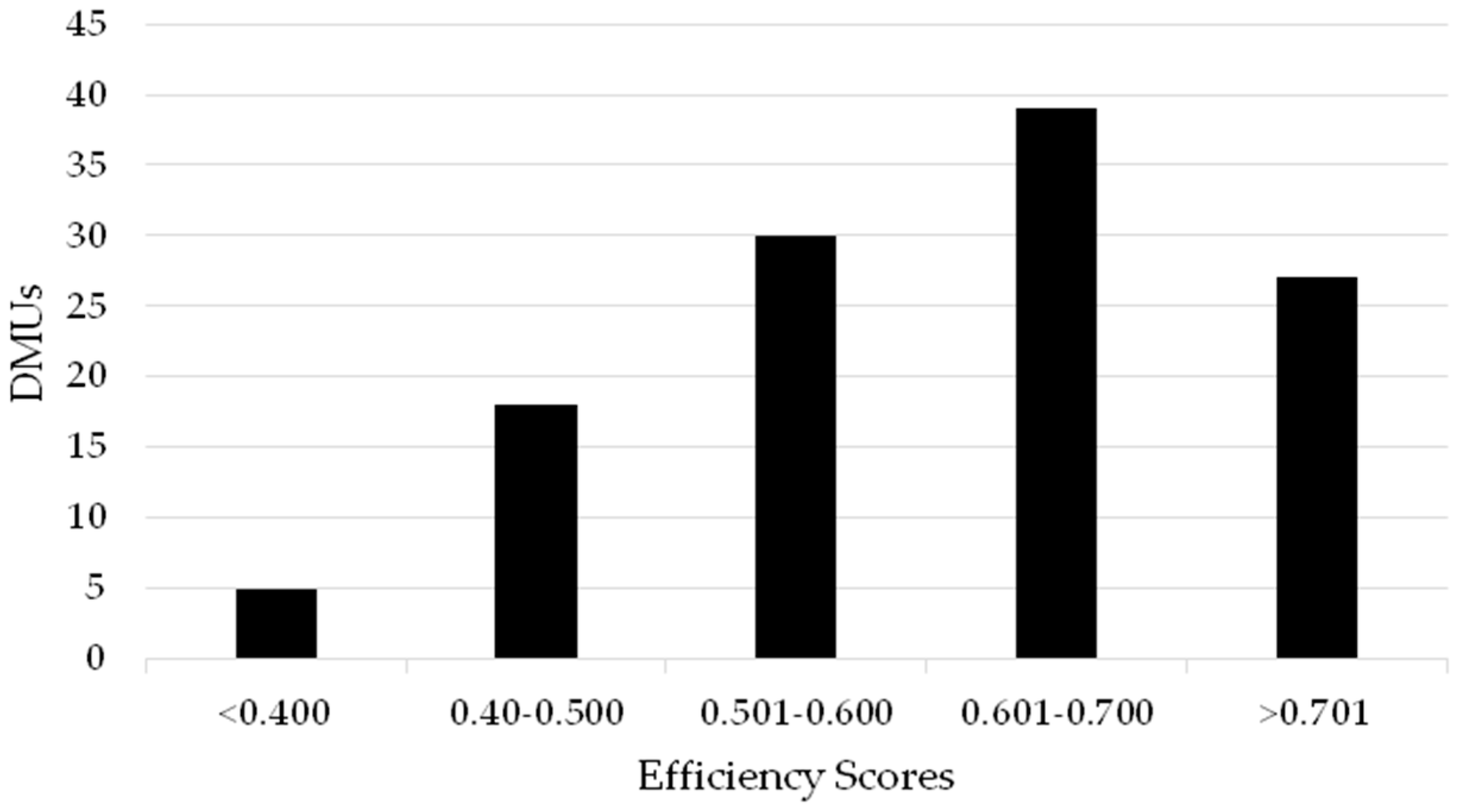
3.1. Environmental Efficiency Evaluation

Figure 2 shows the evaluation results of the environmental efficiency of Chinese open-field grape production. The average overall efficiency score of the 119 counties is 0.651, which indicates that the efficiency in open-field grape production systems in China is relatively low. Additionally, it can be seen from Figure 2 that counties with high efficiency scores are concentrated in the central areas of China, such as the counties of Ningcheng (0.980), Jianping (0.991), and Kalaqinqi (1.000). These counties mostly concentrated in the provinces of Inner Mongolia, Hebei, and Henan. In addition, there are some counties with lower efficiency scores which are concentrated in the provinces of Sichuan and Yunnan, such as the counties of Longcai (0.443), Binchuan (0.326) and Yongren (0.253).

Then, the distribution of efficiency scores of 119 counties was analyzed. In Figure 3, the efficiency scores are located on the X-axis and the Y-axis represents the number of samples (DMUs). It can be seen from Figure 3 that nearly 40 of the sampled counties (DMUs) were in the efficiency interval of 0.601–0.700, which is also the most concentrated range, followed by the efficiency score interval of 0.501–0.700, where 27 DMUs obtained good environmental efficiency scores higher than 0.701; the fewest samples had efficiency scores lower than 0.5.

To analyze the environmental efficiency of open-field grape production systems on a larger scale, the 119 counties were divided into five main production areas. The average efficiency scores and standard deviations (S.D.) are shown in

Table 3. The average efficiency score (AES) of the five areas and the provincial-level regions.

Areas	AES	S.D.	Regions	AES
North China	0.714	0.121	Beijing	0.779
			Shanxi	0.689
			Shandong	0.684
			Henan	0.679
			Hebei	0.772
			Inner Mongolia	0.681
Southwest China	0.528	0.163	Sichuan	0.483
			Yunnan	0.573
Northeast China	0.626	0.158	Heilongjiang	0.564
			Liaoning	0.679
			Jilin	0.635
South China	0.618	0.179	Jiangsu	0.646
			Hubei	0.518
			Anhui	0.669
			Fujian	0.585
			Guangxi	0.673
Northwest China	0.679	0.023	Gansu	0.690
			Xinjiang	0.695
			Shanxi	0.682
			Ningxia	0.650

. It can be seen that the average environmental efficiency of the North China area is 0.714 (S.D.: 0.121), which is the highest efficiency score, followed by Northwest China with 0.679 (S.D.: 0.023), and Northeast China with 0.626 (S.D.: 0.158). South and Southwest China’s environmental efficiency scores are only 0.618 (S.D.: 0.179) and 0.528 (S.D.: 0.163), respectively.

3.2. Global Spatial Correlation Analysis

As the basis and premise of spatial autocorrelation analysis, only the correct and reasonable selection of the spatial weight matrix can be used for the analysis of the spatial correlation. Generally speaking, the spatial weight matrix can be divided into two kinds of matrices, which are “adjacency” and “distance” [49]. In order to distinguish the spatial difference between counties better, the research area is designated as the county administrative regions in this study. The spatial weight matrix of “adjacency” is not suitable because the sampled administrative areas are not adjacent geographically; therefore, the weight of the K-nearest neighbor is selected as the spatial weight to ensure that each administrative region has four areas which are adjacent.

This study measured the global spatial correlation of the environmental efficiency of open-field grape production in China using ArcGIS 10.0 software (ESRI, Redlands, CA, USA) from the American ESRI Company and OpenGeo-Da software (University of Illinois at Urbana-Champaign, Champaign, IL, USA) which is a free software package that was developed by the Spatial Analysis Laboratory of the University of Illinois at Urbana-Champaign under the direction of Luc Anselin. The results of the Global Moran’s I index are shown in

Table 4. Calculated results of the Global Moran’s I.

Year	Moran’s I	p-Value	Z-Value
2014	0.329	0.001	5.784

. The p-value shows that the probability of having a random distribution is very low; hence, spatial autocorrelation exists in the sampled counties. The Moran’s I index is 0.329; the positive index shows that the environmental efficiency has the characteristic of positive spatial autocorrelation. The Z-value and the Moran’s I index also show that similar samples are spatially clustered.

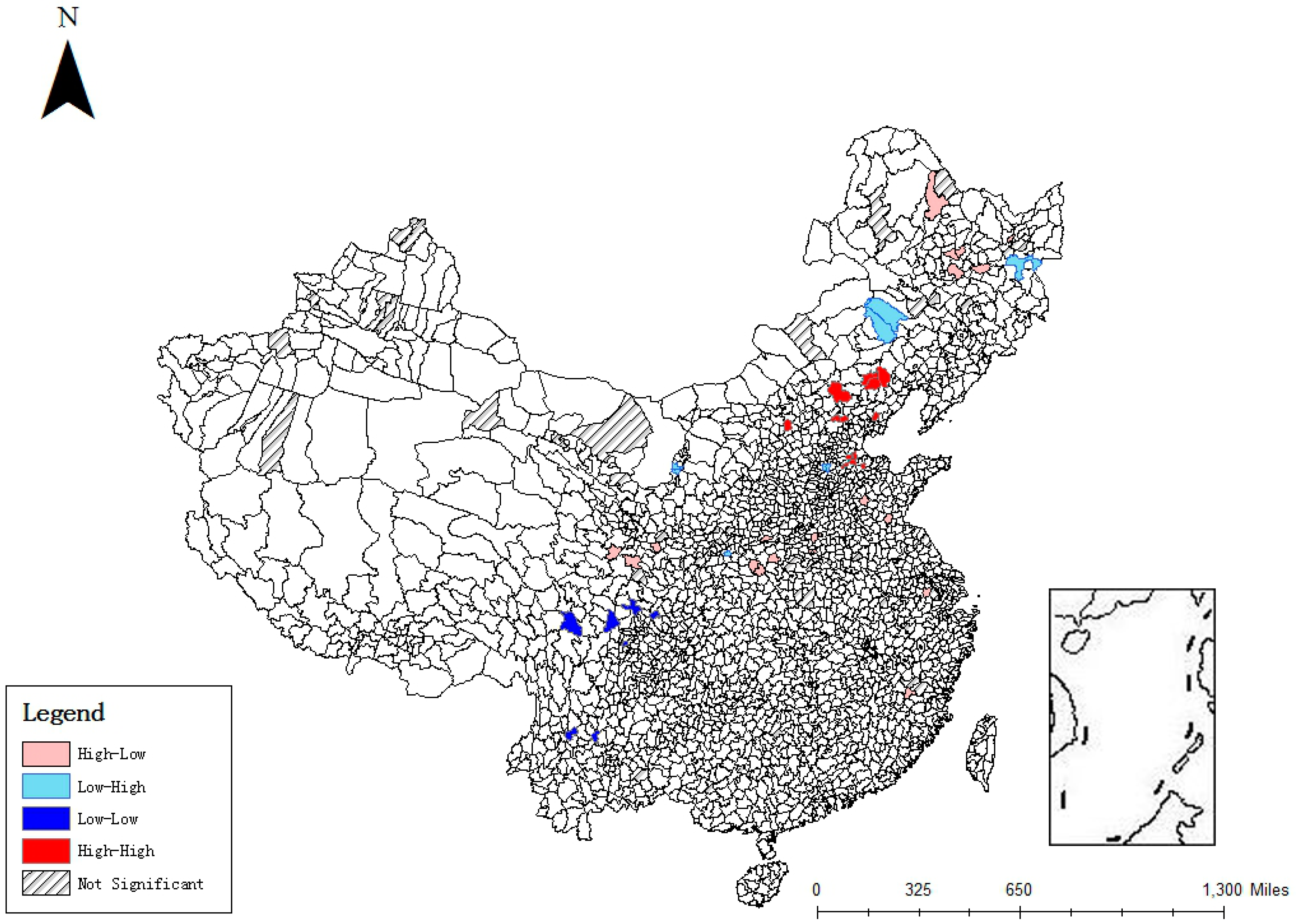
3.3. Local Spatial Correlation Analysis

The spatial autocorrelation of the environmental efficiency of Chinese open-field grape production was evaluated by local indicators of spatial association (LISA). The LISA graph is a vivid and explicit display of the local Moran’s I index. It can show the similarity degree of the attribute values of adjacent areas [50]. The LISA graph is shown in Figure 4, which shows the clustered points of environmental efficiency at the county level in China, respectively, in terms of the four types of spatial correlations: H-H, L-L, H-L, and L-H.

4. Discussion

Figure 2 indicates that efficiency in open-field grape production in China is relatively low. The samples with higher environmental efficiencies are mostly concentrated in the provinces of Inner Mongolia, Hebei, and Henan. The open-field grape vineyards in these counties perform well and profit from many aspects, such as the implementation of technological innovation, or the superior natural conditions for open-field viticulture. The vineyards with lower efficiency scores, which are concentrated in the provinces of Sichuan and Yunnan, show the necessity of reducing resource consumption or carbon emissions for open-field grape production in these counties.

The distribution of efficiency scores in Figure 3 shows that more than 50% of the samples’ environmental efficiencies are less than 0.700. This means that the environmental performance of Chinese open-field grape production systems is inadequate in resource-saving and carbon emissions reduction. In order to obtain higher economic benefits, massive amounts of input resources are applied in the open-field grape industry, such as chemical fertilizers, pesticides, and so on. Such excessive applications of fertilizers and pesticides do not contribute sufficiently to achieving ideal output, but cause serious environmental pollution. In other words, there is a great potential to reduce resource consumption and carbon emissions in these counties and to increase the yield of grapes by implementing structure adjustments and technical innovation, rather than higher inputs.

From the perspective of the production regions, the environmental performance of North China in the open-field grape production system is the best, which also confirms the fact that the north regions develop relatively better in the open-field grape industry, and they are the traditionally suitable viticulture areas as they have appropriate natural conditions for grape growing. Nevertheless, South and Southwest China are non-suitable areas for grape production in terms of natural resources; they have become viable for viticulture nowadays with the improvement of cultivation technology and the appearance of new cultivation patterns. It was also found that, in the same production areas, the regions present obvious differences in environmental efficiency, which can be explained by the fact that the level of open-field grape production development of regions in the same area is not balanced.

The global spatial autocorrelation evaluation results prove that the environmental efficiency of Chinese open-field grape production areas has obvious continuity in neighboring regions and spatial correlation, namely for counties with high environmental efficiency, where the environmental efficiency of the surrounding counties is relatively high. The opposite applies for the regions with low environmental efficiency. The main reason for this phenomenon in the country is that geographical and natural factors result in greatly differing viticulture conditions in different production areas, and the input and output statuses are similar in geographically adjacent areas, so it is easy to form a certain degree of spatial agglomeration.

Figure 4 shows that only 13 counties belong to the H-H type, mainly occurring in the province of Hebei and the city of Beijing. The reason is that the counties with better environmental efficiency invest more in advanced technologies which save materials and operate with lower emissions. On the other hand, the grape growers in these counties affect each other, and better production models will be imitated and promoted by growers to achieve a higher yield of grape. The counties belonging to the L-L type are mainly located in the provinces of Sichuan and Yunnan. These counties are located in Southwest China, which belongs to the emerging areas of open-field grape planting. The growers in these counties tend to use larger amounts of materials, such as fertilizer and pesticides, to gain higher economic benefit. Such an approach leads to higher emissions and resource consumption. Additionally, a more efficient production model is absent in the adjacent area, which contributes to the formation of the agglomeration area with low environmental efficiency. Furthermore, there are some counties that belong to the H-L and L-H types. In these cases, the growers in the counties with low scores are relatively ready to accept more efficient production models. However, changing the production model requires a long time, so low scores and high scores will co-exist in the short term. On the other hand, some growers relying heavily on traditional cultivated experience might not have the will to master new environmental technology, which will lead to a lower score. This is a reason why counties with the H-L and L-H types gather together.

5. Conclusions

In this paper, we aimed at measuring the environmental efficiency of open-field grape production in China based on the SBM model. In addition, spatial relations of environmental efficiency in different grape production counties were studied using spatial econometric methods.

In this paper, our findings have made specific academic and practical contributions.

Firstly, based on the academic findings on the environmental efficiency of China’s open-field grape production [51], the present study further accumulates knowledge in this realm by adding more relevant variables, such as carbon emissions, as the undesirable output variables in this paper. The average environmental efficiency score of grape production in China is 0.651, a result which indicates that China is faced with a relatively low efficiency in open-field grape production. This result is in accordance with the findings of a previous study by Ma [52]. For the improvement of environmental efficiency, more internal potential should be explored, producers’ technology levels should be improved, and the allocation structure of resources should be optimized, rather than simply increasing the inputs, for the sake of reducing the carbon emissions of the production system.

Secondly, this study has practical contributions that benefit open-field grape production in China. According to the phenomenon of spatial agglomeration, the results imply that the environmental efficiency of Chinese open-field grape production areas has obvious continuity in neighboring regions and spatial correlation, and great differences among counties of open-field grape production exist in China in terms of natural conditions. Thus, grape farmers should select the appropriate production mode and input resources based on local circumstances from the perspective of sustainable development. Additionally, the local spatial correlation analysis indicates that it is necessary to pay more attention to the spatial correlation of Chinese open-field grape production areas so as to coordinate the development of the economy and environment in different production areas, which is also important for policy-makers in China.

It should be noted that the data collected for our paper is only for the year 2014, so extending the empirical study to multiple years and further conducting a dynamic analysis of open-field grape production in China may be a particular direction for future research.

References

1. Schandl, H.; Hatfield-Dodds, S.; Wiedmann, T. Decoupling global environmental pressure and economic growth: Scenarios for energy use, materials use and carbon emissions. J. Clean. Prod. 2015, 30, 49–50. [Google Scholar] [CrossRef]
2. Change, C. Intergovernmental Panel on Climate Change; World Meteorological Organization: Geneva, Switzerland, 2007. [Google Scholar]
3. CARS-30, Chinese Agricultural Research System-Grape Industry. Available online: http://119.253.58.231 (accessed on 13 October 2016).
4. Ozkan, B.; Fert, C.; Karadeniz, C.F. Energy and cost analysis for greenhouse and open-field grape production. Energy 2007, 32, 1500–1504. [Google Scholar] [CrossRef]
5. Nadia, M.; Margherita, P.; Valentina, N. Sustainability indicators for environmental performance and sustainability assessment of the productions of four fine Italian wines. Int. J. Sustain. Dev. World Ecol. 2003, 10, 275–282. [Google Scholar]
6. Steenwerth, K.L.; Strong, E.B.; Greenhut, R.F. Life cycle greenhouse gas, energy, and water assessment of wine grape production in California. Int. J. Life Cycle Assess. 2015, 20, 1243–1253. [Google Scholar] [CrossRef]
7. Si, J.T.; Li, D.; Liu, J.W. Study on Methodologies Used to Assess Hazardous Waste Treatment and Management Technologies. Res. Environ. Sci. 2005, 18, 39–42. [Google Scholar]
8. Diego, I.; Almudena, H.; María, T.M. Benchmarking environmental and operational parameters through eco-efficiency criteria for dairy farms. Sci. Total Environ. 2011, 409, 1786–1798. [Google Scholar]
9. Notarnicola, B.; Tassielli, G.; Renzulli, P.A. Environmental and technical improvement of a grape must concentration system via a life cycle approach. J. Clean. Prod. 2014, 89, 87–98. [Google Scholar] [CrossRef]
10. Fuchsz, M.; Kohlheb, N. Comparison of the environmental effects of manure- and crop-based agricultural biogas plants using life cycle analysis. J. Clean. Prod. 2015, 86, 60–66. [Google Scholar] [CrossRef]
11. Parker, P. An Environmental Measure of Japan’s Economic Development: The Ecological Footprint. Geogr. Z. 1998, 86, 106–119. [Google Scholar]
12. Jorgenson, A.K. Consumption and Environmental Degradation: A Cross-National Analysis of the Ecological Footprint. Soc. Probl. 2003, 50, 374–394. [Google Scholar] [CrossRef]
13. Blasi, E.; Passeri, N.; Franco, S. An ecological footprint approach to environmental-economic evaluation of farm results. Agric. Syst. 2016, 145, 76–82. [Google Scholar] [CrossRef]
14. Carolyn, H.; Richard, O.; Daniel, M. Material Flow Analysis: A tool to support environmental policy decision making. Case-studies on the city of Vienna and the Swiss lowlands. Local Environ. 2000, 5, 311–328. [Google Scholar]
15. Kotani, K.; Masunaga, S. Environmental impact assessment of chlorine in liquid crystal display glass (LCDG) based on material flow analysis. J. Environ. Manag. 2012, 112, 304–308. [Google Scholar] [CrossRef] [PubMed]
16. Montanari, R. Environmental efficiency analysis for enel thermo-power plants. J. Clean. Prod. 2004, 12, 403–414. [Google Scholar] [CrossRef]
17. Semenyutina, A.V.; Podkovyrov, I.U.; Semenyutina, V.A. Environmental efficiency of the cluster method of analysis of greenery objects decorative advantages. Life Sci. J. 2014, 11, 699–701. [Google Scholar]
18. Reinhard, S.; Lovell, C.; Thijssen, G.J. Environmental efficiency with multiple environmentally detrimental variables; estimated with SFA and DEA. Eur. J. Oper. Res. 2000, 121, 287–303. [Google Scholar] [CrossRef]
19. Power, B.; Cacho, O.J. Identifying risk-efficient strategies using stochastic frontier analysis and simulation: An application to irrigated cropping in Australia. Agric. Syst. 2014, 125, 23–32. [Google Scholar] [CrossRef]
20. Waryanto, B.; Chozin, M.A.; Dadang. Environmental Efficiency Analysis of Shallot Farming: A Stochastic Frontier Translog Regression Approach. J. Biol. Agric. Healthc. 2014, 19, 87–100. [Google Scholar]
21. Katharakis, G.; Katharaki, M.; Katostaras, T. An empirical study of comparing DEA and SFA methods to measure hospital units’ efficiency. Int. J. Oper. Res. 2014, 21, 242–251. [Google Scholar] [CrossRef]
22. Vencheh, A.H.; Matin, R.K.; Kajani, M.T. Undesirable factors in efficiency measurement. Appl. Math. Comput. 2005, 163, 547–552. [Google Scholar] [CrossRef]
23. Sueyoshi, T.; Goto, M. DEA radial measurement for environmental assessment: A comparative study between Japanese chemical and pharmaceutical firms. Appl. Energy 2014, 115, 502–513. [Google Scholar] [CrossRef]
24. Halkos, G.E.; Tzeremes, N.G. Measuring the effect of Kyoto protocol agreement on countries’ environmental efficiency in CO2 emissions: An application of conditional full frontiers. J. Prod. Anal. 2014, 41, 367–382. [Google Scholar] [CrossRef] [Green Version]
25. Skevas, T.; Stefanou, S.E.; Lansink, A.O. Pesticide use, environmental spillovers and efficiency: A DEA risk-adjusted efficiency approach applied to Dutch arable farming. Eur. J. Oper. Res. 2014, 237, 658–664. [Google Scholar] [CrossRef]
26. Vlontzos, G.; Niavis, S.; Manos, B. A DEA approach for estimating the agricultural energy and environmental efficiency of EU countries. Renew. Sustain. Energy Rev. 2014, 40, 91–96. [Google Scholar] [CrossRef]
27. Valadkhani, A.; Roshdi, I.; Smyth, R. A multiplicative environmental DEA approach to measure efficiency changes in the world’s major polluters. Energy Econ. 2016, 54, 363–375. [Google Scholar] [CrossRef]
28. Wang, X.; Huang, G. Impacts assessment of air emissions from point sources in Saskatchewan, Canada—A spatial analysis approach. Environ. Prog. Sustain. Energy 2014, 34, 1–10. [Google Scholar] [CrossRef]
29. Camarero, M.; Picazo-Tadeo, A.J.; Tamarit, C. Is the environmental performance of industrialized countries converging? A ‘SURE’ approach to testing for convergence. Ecol. Econ. 2008, 66, 653–661. [Google Scholar] [CrossRef]
30. Marconi, V.; Raggi, M.; Viaggi, D. Assessing the impact of RDP agri-environment measures on the use of nitrogen-based mineral fertilizers through spatial econometrics: The case study of Emilia-Romagna (Italy). Ecol. Indic. 2015, 59, 27–40. [Google Scholar] [CrossRef]
31. Costantini, V.; Mazzanti, M.; Montini, A. Environmental performance, innovation and spillovers. Evidence from a regional NAMEA. Ecol. Econ. 2013, 89, 101–114. [Google Scholar] [CrossRef]
32. Adetutu, M.; Glass, A.J.; Kenjegalieva, K. The effects of efficiency and TFP growth on pollution in Europe: A multistage spatial analysis. J. Prod. Anal. 2015, 43, 307–326. [Google Scholar] [CrossRef] [Green Version]
33. Shen, N.; Wang, Q.W. Environmental Efficiency Evaluation and Spatial Effect Taking Account of Technology Heterogeneity. J. Ind. Eng. Eng. Manag. 2015, 29, 162–168. [Google Scholar]
34. Zhao, D.L. Empirical Research on the Evaluation and Spatial Correlation of Industrial Environmental Efficiency in China. Master’s Thesis, Beijing Forestry University, Beijing, China, 2015. [Google Scholar]
35. Wu, J.; Zhu, Q.; Chu, J. Measuring energy and environmental efficiency of transportation systems in China based on a parallel DEA approach. Transp. Res. Part D Transp. Environ. 2016, 48, 460–472. [Google Scholar] [CrossRef]
36. Wang, H.B.; Wang, X.D.; Wang, B.L. Present situation, problems and Development Countermeasures of grape industry in northern China. Agric. Eng. Technol. (Greenh. Hortic.) 2011, 1, 21–24. [Google Scholar]
37. Wei, T.; Lujia, Y.; Jing, J. Research on Chinese agricultural eco-efficiency based on SBM model of undesirable outputs. China Rural Surv. 2014, 5, 59–71. [Google Scholar]
38. West, T.O.; Marland, G. A synthesis of carbon sequestration, carbon emissions, and net carbon flux in agriculture: Comparing tillage practices in the United States. Agric. Ecosyst. Environ. 2002, 91, 217–232. [Google Scholar] [CrossRef]
39. Lal, R. Carbon emission from farm operations. Environ. Int. 2004, 30, 981–990. [Google Scholar] [CrossRef] [PubMed]
40. Dyer, J.A.; Desjardins, R.L. Simulated farm fieldwork, energy consumption and related greenhouse gas emissions in Canada. Biosyst. Eng. 2003, 85, 503–513. [Google Scholar] [CrossRef]
41. Pishgar-Komleh, S.H.; Ghahderijani, M.; Sefeedpari, P. Energy consumption and CO2 emissions analysis of potato production based on different farm size levels in Iran. J. Clean. Prod. 2012, 33, 183–191. [Google Scholar] [CrossRef]
42. Lampe, H.W.; Hilgers, D. Trajectories of efficiency measurement: A bibliometric analysis of DEA and SFA. Eur. J. Oper. Res. 2015, 240, 1–21. [Google Scholar] [CrossRef]
43. Martínez, C.I.P. Estimating and Analyzing Energy Efficiency in German and Colombian Manufacturing Industries Using DEA and Data Panel Analysis. Part I: Energy-intensive Sectors. Energy Sources Part B Econ. Plan. Policy 2015, 10, 322–331. [Google Scholar] [CrossRef]
44. Saati, S.; Memariani, A. SBM model with fuzzy input-output levels in DEA. Aust. J. Basic Appl. Sci. 2009, 3, 352–357. [Google Scholar]
45. Tone, K. A slacks-based measure of efficiency in data envelopment analysis. Eur. J. Oper. Res. 2001, 130, 498–509. [Google Scholar] [CrossRef]
46. Zheng, J.; Liu, X.; Bigsten, A. Ownership structure and determinants of technical efficiency: An application of data envelopment analysis to Chinese enterprises (1986–1990). J. Comp. Econ. 1998, 26, 465–484. [Google Scholar] [CrossRef]
47. Diniz-Filho, J.A.F.; Bini, L.M.; Hawkins, B.A. Spatial autocorrelation and red herrings in geographical ecology. Glob. Ecol. Biogeogr. 2003, 12, 53–64. [Google Scholar] [CrossRef]
48. LeSage, J.P. An introduction to spatial econometrics. Revue D’économie Industrielle 2008, 123, 19–44. [Google Scholar] [CrossRef]
49. Aldstadt, J.; Getis, A. Using AMOEBA to Create a Spatial Weights Matrix and Identify Spatial Clusters. Geogr. Anal. 2006, 38, 327–343. [Google Scholar] [CrossRef]
50. Anselin, L. Local Indicators of Spatial Association—LISA. Geogr. Anal. 1995, 27, 93–115. [Google Scholar] [CrossRef]
51. Mu, W.; Yan, Z.; Gavrila, S.P. A Full Carbon Cycle Comparative Analysis in Greenhouse and Open-Field Grape Cultivation. J. Environ. Prot. Ecol. 2015, 16, 461–469. [Google Scholar]
52. Ma, C.Y.; Mu, W.S. Assessing the technical efficiency of grape production in open field cultivation in China. J. Food Agric. Environ. 2012, 10, 345–349. [Google Scholar]
Figure 1. The production process of open-field grapes under the constraint of carbon emissions.
Sustainability 08 01246 g001
Figure 2. Efficiency evaluation results of Chinese open-field grape production.
Sustainability 08 01246 g002
Figure 3. Efficiency score distribution of Chinese open-field grape production.
Sustainability 08 01246 g003
Figure 4. The LISA graph of the environmental efficiency of Chinese open-field grape production.
Sustainability 08 01246 g004