1. Introduction
In general, most scheduling problems usually involve multiple objectives like cost, tardiness, and earliness due to demand of practical production and these objectives are often conflicting with each other, which is a challenging task for solving the optimal solution [
1]. Thus, study of the multi-objective scheduling problem is very important in terms of theoretical significance and applying value. In recent years, many manufacturing companies and researchers have started to focus on the minimum energy consumption [
2]. Just-in-time (JIT) production is another key issue because most companies are concerned not only with reducing inventory cost but also with delivering on time. It is noted that there is a remarkable relation between JIT scheduling problems and controllable processing times, since the scheduling environment can approach JIT philosophy by controlling the process times [
3]. The controllable processing times mean that each operation can be processed in a reasonable shorter or longer time by allocating the available resources like fuel, equipment, catalyzes, manpower and so on. The mentioned-above factors (i.e., energy consumption and JIT) directly affect the production efficiency. Therefore, energy consumption and JIT production should be taken into account simultaneously in manufacturing sectors.
The energy consumption problem is driven by the fact that the pressing campaign of sustainable development is now widely accepted in real production systems. “Rising energy consumption has triggered some negative impacts on environment which has led to legislative restrictions on manufacturing companies” [
4]. Obviously, the current trend of green manufacturing has brought about new pressures and challenges for manufacturing enterprises. Consequently, “enterprises have to reduce energy consumption so as to save cost and become more environmentally friendly”. Most researches on minimizing energy consumption largely concentrate on more energy efficient machines or machine process plans. However, the majority of energy consumption is not directly related to the production of components [
5]. Drake et al. [
6] further proved that there existed significant energy consumption when a machine is idle but still runs. Therefore, minimization of energy consumption can be realized by turning off/on the machine between scheduled jobs rather than keeping the machine idle. Compared with machine or process redesign, this turn off/on strategy only needs a little financial investment and can easily be implemented.
JIT production also plays a key role in manufacturing sectors since a scheduling scenario based on JIT philosophy can effectively reduce cost and improve reputation of companies among the customers [
7]. JIT philosophy in manufacturing systems has been studied widely in the scheduling field, especially for those with earliness and tardiness (E/T) problems. In the JIT environment, tasks which are finished before their due date may incur earliness penalties such as inventory cost while a tardy task can cause customer dissatisfaction, lost sales and loss of reputation. Therefore, a desirable schedule is one where all jobs are completed exactly on their own due dates. In reality, JIT scheduling can be achieved by controlling job processing times. Although job processing times in most literatures are fixed positive parameters, it is now accepted that in practice the scheduler can change processing times by increasing or reducing additional resources. Therefore, controllable processing times can try to ensure that all jobs can be processed on their own due dates, which can increase profit by squeezing inventory cost and improving customer satisfaction.
Most conventional scheduling problems use production efficiency, cost and quality as their preeminent optimization objectives. However, because of increasing costs of energy and environmental pollution, “low-carbon scheduling” as a novel scheduling model has received increasing attention from scholars and engineers [
8]. Based on the discussion above, many researchers and manufacturing companies realize the importance of energy efficiency. To the best of the authors’ knowledge, the single machine scheduling problem with controllable processing and setup times, including energy consumption conception, still has not been studied in the previous researches reported. Furthermore, this addressed scheduling is not only a multi-objective optimization problem (MOP) in nature but also a NP-hard problem. Multi-objective evolutionary algorithm (MOEA) is very suitable to solve this kind of problem because MOEA can obtain the non-dominated solutions in a single run and is also applied successfully in the optimization field [
9,
10,
11,
12,
13,
14]. This motivates us to develop a new multi-objective scheduling model and propose a MOEA to cope with this type of problem.
For a single-machine scheduling environment, Mouzon et al. [
15] proposed a multi-objective mathematical programming model and several algorithms for a single Computer numerical control (CNC) machine scheduling problem with the goals of reducing both energy consumption and total completion time. Mouzon and Yildirim [
16] applied a greedy randomized adaptive search algorithm to a single-machine multi-objective optimization scheduling problem with the objective of minimizing the total energy consumption and total tardiness. Rager et al. [
2] proposed an evolutionary algorithm for energy-oriented parallel machine scheduling. For the flow-shop environment, Fang and Uhan et al. [
17,
18] presented some new mathematical programming models of its scheduling problem that consider “peak power load, energy consumption, and associated carbon footprint in addition to cycle time”. Bruzzone et al. [
19] proposed an approach that relies on a mixed-integer programming model in which the reference schedule was modified by an advanced planning and scheduling (APS) system to consider energy consumption without changing the jobs’ assignments and sequencing. Dai et al. [
20] proposed an energy-efficient model for flexible flow-shop scheduling and developed a genetic-simulated annealing algorithm to solve it. Luo et al. [
21] proposed a new ant colony optimization meta-heuristic for production efficiency and electric power cost for a hybrid flow shop scheduling problem. Keller et al. [
22] developed a heuristic method for the hybrid flow-shop scheduling problem considering energy flexibility. For the job-shop scheduling environment, Liu et al. [
23] developed a multi-objective scheduling method for the classical job-shop scheduling problem (JSP) with total energy consumption and total weighted tardiness as objectives. Kang et al. [
24,
25] to address a selected problem two approaches are investigated, i.e., traditional scheduling algorithms and genetic algorithms based multi-objective optimization, both approaches are compared based given key performance indicators, computational time required and the quality of generated schedule.
In this work we mainly study on a single machine scheduling with controllable processing and setup times for minimizing production costs (i.e., cost and total E/T) and energy consumption. These objectives are important Key Performance Indicators (KPIs) for enterprises. The purpose of our current study is to develop a MOEA called local MOEA (LMOEA) to obtain trade-offs between the three objectives closer towards true Pareto front. According to the features of the addressed problem and evolutionary algorithm, this proposed LMOEA uses a new encode mechanism which can convert discrete optimization problems into continuous optimization problems, and adopts a hybrid local search with three different strategies to enhance exploitation ability.
The remainder of the paper is organized as follows. In
Section 2, we give a review on scheduling problems considering energy consumption and JIT scheduling with controllable processing time. In
Section 3, we describe a formal definition of the addressed problem. Then, we proposed a MOEA with multiple local search operators for handling the scheduling problem in
Section 4. The experimental results of our proposed LMOEA are presented and analyzed in
Section 5. In
Section 6, we give a case study. Concluding remarks and suggestions for several future research subjects are given in
Section 7.
4. The Proposed LMOEA for Multi-Objective Scheduling with Controllable Processing Times
In this section, firstly we state the basic background on multi-objective optimization, and then describe the framework of the proposed LMOEA. Finally, some main operators are presented in detail for optimizing the scheduling problem.
4.1. Background on Multi-Objective Optimization
To better understand our proposed LMOEA for solving the above problem, we begin with a brief introduction of basic concept of MOEA. Without loss of generality, we assume that there are several objectives to be minimized simultaneously. A multi-objective optimization problem (MOP) is composed of multiple conflicting objectives. In general, a MOP can be defined in the following form [
44].
where
x is called a decision vector and Ω is the search space.
f(
x) constitutes
k individual objective functions.
Let a and b ϵ Ω, a vector a = is said to dominate another vector b (denoted by a b) if and only if for each i ϵ {1,…, k} and for at least index j ϵ {1,…, k}. A solution x* ϵ Ω is called a Pareto optimal solution in Equation (15) if there is not any a solution x ϵ Ω that dominates x*. The corresponding objective function is called Pareto optimal front vector f (x*). That is to say, for a Pareto optimal solution, the improvement of any objective must cause the deterioration of at least another objective. The set of all Pareto optimal solutions is called Pareto set (PS*), while the set of all Pareto optimal front vectors is called the Pareto optimal front (PF*). The main goal of multi-objective optimization is to find PF*. However, in general a Pareto front consists of a large number of points. Therefore, a good Pareto front should contain a limited number of points which should be as close as possible to the PF* and should be uniformly spread as well.
4.2. Framework of the Proposed Algorithm
As described in the previous section, the goal of this work is to develop a hybrid local MOEA (LMOEA) for above multi-objective scheduling problem. In the proposed LMOEA, a more suitable crossover and a more intensive local search are used to keep a better balance between the exploration and exploitation in search space.
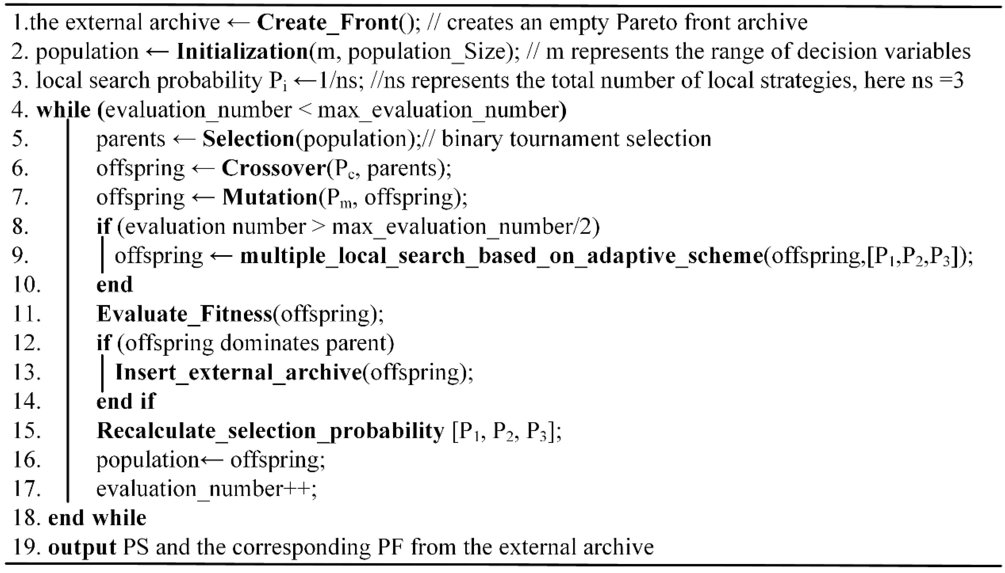
We present two key strategies in the proposed LMOEA for solving this scheduling problem. (1) a new encoding scheme based on a real number to convert discrete problems into continuous problems; (2) the multiple local search strategies based self-adaptive selection scheme to make the candidate solution approach toward an optimal solution. The first strategy is used in solution representation to encode and decode solutions. The second strategy is performed on offspring solutions after crossover and mutation operation so as to exploit better solution in offspring’s neighborhood. The pseudocode of the proposed LMOEA is shown in
Figure 2.
Section 4.2.2 gives detailed illustration on line 6 of
Figure 2.
Section 4.2.3 also provides some explanations on line 7.
Section 4.2.4 describes a concrete principle of the local search on line 8–10 in
Figure 2. The calculation of each local search strategy rate on line 15 is also stated in
Section 4.2.4. It is pointed out that the local search strategy takes much computation time during search process, even though it has a positive effect on the behavior of the LMOEA. So we execute the local search strategy in later stage (namely half of max function evaluation number) to establish a balance between the time consumption and search accuracy.
Section 4.2.5 gives a detailed description on line 12–14. The external archive is used to store non-dominated solutions found so far. To maintain the diversity of the no-dominated solutions in the external archive, the crowding distance technique is adopted to discard the solutions with worse crowding distance when the number of non-dominated solutions exceeds the size of the external archive.
Additionally, there are three crucial differences between our proposal and the previous researches on the hybrid MOEAs.
According to the no free lunch theorem, one algorithm cannot obtain a better result than all the others on all problems. Therefore, the proposed MOEA combines multiple techniques including harmony search (HS), genetic algorithm (GA), and differential evolution (DE) strategy. Even though the three nature-inspired algorithms are all population-based metaheuristics, they have different search manners or directions in search space, which can improve the diversity of the population and stability of the algorithm. The reasons why we adopt these three strategies in our proposal are explained in
Section 3.2.1.
The proposed algorithm is based on multiple techniques consisting of HS, GA, and DE, so it needs to use a new hybrid selection scheme to automatically select an appropriate operation during the search process. This new hybrid selection mechanism is featured because the static and adaptive selection scheme can switch alternately. The aim of this hybrid selection mechanism is to avoid adopting the same search operator over the course of the iteration, which means the search process get trapped in the local optima. Therefore, by integrating the advantages of static and adaptive selection scheme, this hybrid selection can help the algorithm to mitigate the local optima and search for preferable solutions in unexplored areas.
In the following subsections, the ingredients of our proposed algorithm are detailed, including a new representation for this scheduling problem, crossover operator, mutation operator, the multiple local search approaches based on self-adaptive mechanism, and replacement strategy.
4.2.1. Representation
One of the important issues in applying MOEA to the considered problem lies in its solution representation. According to the feature of problem and algorithm considered, we present a new encoding scheme (solution representation) based on the real number for this scheduling problem in this work. This solution representation is different from literatures [
45,
46]. In [
45], the length of solution representation developed by them is 2
n (
n is the number of jobs), while our proposal is
n. In [
46], they adopted the largest position value (LPV) rule to denote order of job process in solution representation. Whereas our representation contains more information. This encoding scheme we proposed has three advantages as follows.
- (1)
Chromosome structure is simpler. Even though this proposed encoding scheme only consists of one dimensional structure, it contains two contents namely amount of compression or expansion of job processing times and job sequence.
- (2)
Problem solving is simpler. Discrete optimization problems can be converted to continuous optimization problems by adoption of the proposed encoding scheme.
- (3)
Constraint handling mechanism is simpler even unnecessary. The algorithm with the conventional encoding scheme needs to employ some special recombination operators to avoid unfeasible solution. However, this approach with the proposed encoding mechanism can generate feasible solutions.
The main principle of this encoding scheme is as follows. For a given
n jobs,
n real values, denoting amount of compression or expansion and job sequence, are randomly created from a uniform distribution in its own range (
mc,
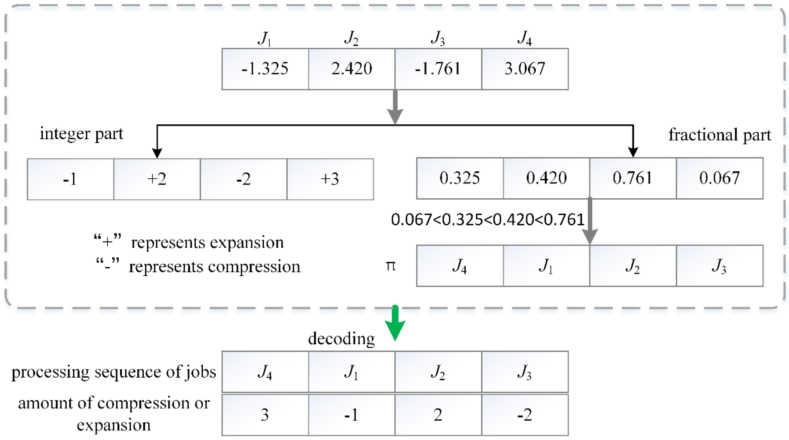
me). The integer part, obtained by rounding off this real value, stands for the actual amount of compression or expansion of job processing times. To distinguish compression and expansion of job processing time, the positive integer represents actual amount of expansion and the negative integer denotes actual amount of compression. It is noted that the positive and negative number are generated with equal probability. The fractional part of a real number implies the processing order of jobs on a single machine. To further describe the proposed encoding scheme,
Figure 3 illustrates the solution representation. For a given single machine scheduling problem with four jobs, we assume that its maximum amount of compression and expansion are
mc = (−3, −4, −2, −4) and
me = (2, 3, 2, 4), respectively. One chromosome vector (−1.325, 2.420, −1.761, 3.067) is randomly generated in the range of compression or expansion amount. This chromosome can be translated into two meanings: (1) actual amount vector of compression or expansion of job processing times
m = (−1, 2, −2, 3); (2) the sequence of jobs namely π = (
J4,
J1,
J2,
J3). In detail, the integer part (−1, 2, −2, 3) is obtained by rounding off the real number and represents actual amount of compression or expansion of job processing times. Among them, the integer value “−1” in the first position of the integer part means that amount of compression of
J1 is one unit time. Similarly, the value “3” in the fourth position denotes that amount of expansion of
J4 is three unit time. The fractional part (0.325, 0.420, 0.761, 0.067) implies job processing sequence. The fractional part numbers are sorted based on non-descending order, namely 0.067 < 0.325 < 0.420 < 0.761. Accordingly, the corresponding job processing sequence is (
J4,
J1,
J2,
J3). Using this encoding scheme, it is easy to recognize the actual amount of compression or expansion of jobs and processing sequence of jobs. Therefore, this decoding mechanism is very simple and efficient based on the above analysis.
4.2.2. Crossover Operator
Crossover is one of the most vital operators and is utilized to generate the new offspring solutions. It is reasonable that an efficient crossover operator not only update the population but also inherit elite genes of their parents to the offspring individuals. In the past years, many types of crossover operators have been proposed for solving continuous optimization problems, such as uniform crossover [
47], simulated binary crossover (SBX) [
48], blend crossover (BLX-α) [
49], single point crossover, et al. As we know, arithmetic crossovers and permutation-based crossover are more efficient for discrete problems, but they are not suitable for the encoding scheme in this study. In addition, the effectiveness of the crossover operators depends on the specific problems. According to the experimental study on different crossovers for all test instances in
Section 5.4, finally SBX is applied to our proposed LMOEA in this paper.
4.2.3. Mutation Operator
Mutation is also an important operator in MOEA, which can fine-tune some genes with a small probability. Moreover, it helps the algorithm to escape from local optimum as well. In this work, the mutation operator is composed of two kinds of mutation techniques. The goal of the first mutation technique is to adjust compression or expansion amount of job processing times in the range. The second mutation technique called swap mutation operator is used to swap order of jobs. The first mutation technique can achieve its objective by changing integer value in its range. The other technique can exchange the job processing order by swamping two genes’ fractional parts. When performing a mutation operator on an individual, either the first mutation or the second mutation operator is chosen with the possibility of 0.5. To detail the process of this mutation operator, an example of how to implement the hybrid mutation is presented in
Figure 4. For the first mutation operator as shown in
Figure 4a, firstly a mutation position is selected from uniform distribution between 1 and 4. We assume that the second gene is chosen, and then a new integer is generated randomly from its range. For the second mutation operator as shown in
Figure 4b, when the two genes are randomly selected out (e.g., the second and fourth gene), their fractional parts are swamped. More specifically, the original fractional values of the second and fourth genes are 0.420 and 0.067, respectively. The original sequence of jobs is π = (
J4,
J1,
J2,
J3) according to the above proposed encoding scheme. After applying the second mutation operation, the fractional values of the second and fourth genes become 0.067 and 0.420, respectively. Accordingly, the sequence of jobs also becomes π = (
J2,
J1,
J4,
J3) and the corresponding compression or expansion amount of job processing times is
m = (2, −1, 3, −2).
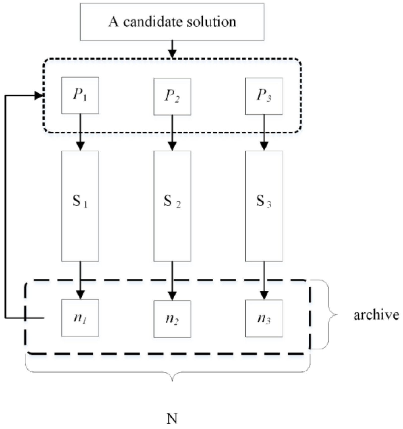
4.2.4. Local Search Procedure
A local search strategy can effectively enhance exploitation ability of the algorithm. In this research, we present three different local search strategies based on self-adaptive selection mechanism to obtain better approximate solutions. For a given schedule, in Strategy 1 (S1), we insert the fractional part randomly chosen into another job position with the biggest setup time to reduce the energy consumption. Strategy 2 (S2) is another local search technique that may minimize the total tardiness/earliness by swapping the largest lateness or earliness of a job with the smaller one. Strategy 3 (S3) can be used to decrease cost by approaching the actual processing times closer toward the corresponding normal processing times. The flow chart of the multiple local search is presented in
Figure 5.
To select an appropriate local search operator for a given schedule, a self-adaptive selection mechanism is utilized. Selection probability of each local search strategy can be obtained by recording the kind of local operator performed by each solution. In initialization, each local search strategy is chosen with the possibility of 1/3. Afterward, when a local search strategy is chosen, the strategy will be assigned to a new solution. Let
Pi denote the selection probability of the
ith strategy and
P1 is probability for S1,
P2 for S2,
P3 for S3. The self-adaptive selection mechanism can be described as follows. Firstly, if the external archive storing non-dominated solution found so far is updated, compute the selection rate of each local strategy
, where
ni is the number of non-dominated solutions obtained by the
ith local strategy in the external archive.
represents the current size of external archive. Then select a strategy by using the roulette wheel approach. To avoid this situation of all candidate solutions adopting the same local search operator during search process, each local strategy will be assigned with the possibility of 1/3 when this situation occurs. Based on the above analysis, this multiple local operator based on self-adaptive mechanism is very simple and effective for solving complex problems. We also investigate the effect of the hybridization of local search on performance of the proposed algorithm in
Section 5.6.
4.2.5. Replacement Strategy
Multi-objective optimization is different from mono-objective optimization. In multi-objective optimization, each solution is associated with a rank equal to its non-dominance level (e.g., 1 for the best level, 2 for the second best level and so on). Then within each level or rank, a crowding distance technique, which indicates the sum of distances to the closest individual along each objective, is used to define an ordering among solutions. To achieve wide spread of the obtained Pareto fronts, a trial solution with large crowding distance is preferred to one with small crowding distance. Our replacement method is based on rank and crowding distance. That is, replace the solution in the external archive if it is dominated by the offspring or both are non-dominate level and the one has the worst crowding distance in the population consisting of solutions from external archive plus offspring. Otherwise the offspring will be discarded. However, at the beginning of update, the external archive is empty and the
PS in initial population is directly inserted into the archive as presented in
Figure 6.
5. Experimental Studies
In the section we conduct a set of computational experiments to evaluate the performance of the proposed LMOEA, which was coded in java and run on a Intel Core i5 1.6 GHz PC with 1 GB memory.
This section is devoted to measuring the performance of the proposed algorithm LMOEA for the addressed problems. In this section, the empirical studies contain the following four aspects.
- (1)
Efficiency comparisons with different crossover in LMOEA for all problems in
Section 5.4.
- (2)
The best choice of crossover rate and mutation rate for all test instances in
Section 5.5.
- (3)
Performance analysis on the local search strategy of the LMOEA for the considered problems in
Section 5.6.
- (4)
Performance comparisons with other MOEAs for the scheduling problems in
Section 5.7.
In the following subsections, test problems, performance metrics and parameter settings are described at first, and then the experimental studies are further investigated step by step.
5.1. Test Instances
Three levels of problem size (i.e., small, medium and large) depending on the number of jobs and stages are considered in this experiment. The due date of each job is
dj =
k ×
pj,
j = 1, 2,…,
n where
k is control factor. The value of
k will be set as 1, 2,…, 5 which corresponds to the trend of less tight due dates. The time unit is minute. The other parameters of data are shown in
Table 2. The following tables record the results obtained by different MOEAs for each instance, where the instance with
n jobs and
k parameter is denoted as symbol “Problem_
n_
k”. For example, “Problem_10_1” represents the addressed problem is featured by 10 jobs and
k equal to 1.
5.2. Performance Metrics
To measure the Pareto front (
PF) obtained by these proposed algorithms, some metrics such as Spread [
44,
50], Generational Distance (GD) [
51], and Inverse Generational Distance (IGD) [
52] should be employed as below.
(1) Spread. The metric is a diversity indicator that measures the extent of spread achieved among the front found. The definition of Spread in [
44] was used for bi-objective problems. As to problems with three or more objectives, the modified Spread is different, as it given in Equation (16) [
50]. The metric is defined as:
where
dfj denotes the Euclidean distance of each point in
PF to its closest point in
PF*,
is the number of vectors in
PF*,
is the Euclidean distance between the extreme solutions in the
ith objective and the boundary solutions of the
PF* obtained, and
is the average of all
.
N is the number of
PF* found. If the metric value is zero, then all the members of Pareto-optimal front are evenly spaced. A smaller value of the metric indicates a better distribution and diversity.
(2) Generational Distance (GD). The GD metric indicates how far the
PF found is from the
PF*. This metric is formulated as:
where
is the number of Pareto front points found so far,
li is the Euclidean distance between the
ith member of
PF obtained and the nearest member of the
PF*. A low GD value is desirable, which denotes a good convergence performance.
(3) Inverse Generational Distance (IGD). It is a variant of the GD but represents a combined or comprehensive indicator. It measures the distances between each solution consisting of the optimal Pareto front and obtained front. It can be defined as follows:
where
H is the number of the optimal Pareto front and
is the Euclidean distance between each point of that front and the nearest member of the approximation. Fronts with lower IGD value are desirable.
It should be noted that the true PF* of the considered problem maybe is unknown, so we regard the Pareto front of all the algorithms in all runs as the Pareto optimal front.
5.3. Parameters Settings
For the proposed LMOEA, the population size and external size are set to 100 and the number of evaluation function is set to 25,000. 30 independent runs are conducted for each algorithm on each test instance.
The optimal results are highlighted with bold in the tables. Since all candidate MOEAs are stochastic algorithms, the following statistical analysis is necessary for providing confidential comparisons. Firstly, the kolmogorov-smirnov test is conducted to check whether the results follow the normal distribution or not. If the results are not normal distributed, the t-test will be used to test the result of each algorithm; otherwise, a Wilcoxon rank sum test is applied to the mean values. The two statistical tests executed on the pairs of the algorithms are to measure the significant differences between the results obtained by different algorithms. The confidence level for all tests is set to 95% (corresponding to a p-value below 0.05). The sign “+” indicates that our proposed LMOEA algorithm performs significantly better than the second best algorithm on average. While “−” represents that the performance of LMOEA algorithm is significantly worse than that of the best algorithm. The “=” sign denotes that there is no significant difference between LMOEA algorithm and the best or second best MOEA. The bottom rows of these tables list the ratio of dominant performance for the corresponding metric. For example, 3/15 indicates the corresponding algorithm outperform its rivals on 3 out of 15 problems for a given metric.
Before solving these scheduling instances, we should select an appropriate crossover operator, crossover and mutation rate for LMOEA in the following
Section 5.4 and
Section 5.5.
5.4. Comparison among Different Crossovers
To determine an appropriate crossover operator among SBX, BLX-α, uniform crossover, and single point crossover, we execute experiments on all instances. There are four versions of LMOEA only adopting SBX, BLX-α, uniform crossover and single point crossover operator. The crossover and mutation rate in these four versions are set to 0.9 and 1/
n (
n is the number of jobs), respectively. We conduct 30 independent runs for each MOEA on each instance and compare average value of IGD, GD, and Spread metric over all runs for different crossover operators as shown in
Figure 7. According to
Section 5.2, the smaller the metric is, the better the performance of the algorithm is. We can clearly observe that the proposed LMOEA with only SBX outperforms its counterparts in terms of the IGD, GD, and Spread metric value. Therefore, the SBX (crossover and mutation distribution index are both 20) operator, regarded as a crossover operator, is introduced into the LMOEA for solving these scheduling instances.
5.5. The Best Choice of Crossover and Mutation Probability
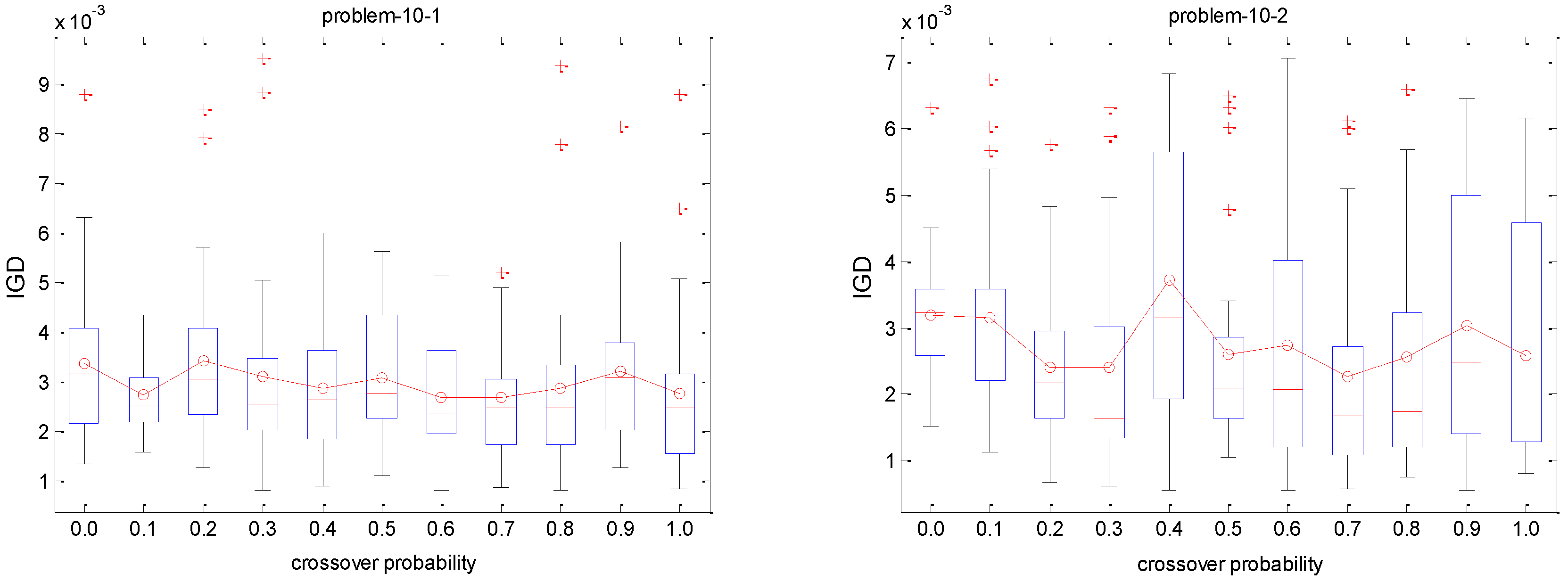
The quality of the algorithm is significantly influenced by the value of crossover and mutation rate. In this subsection we study the performance of the different parameters of LMOEA on all test instances.
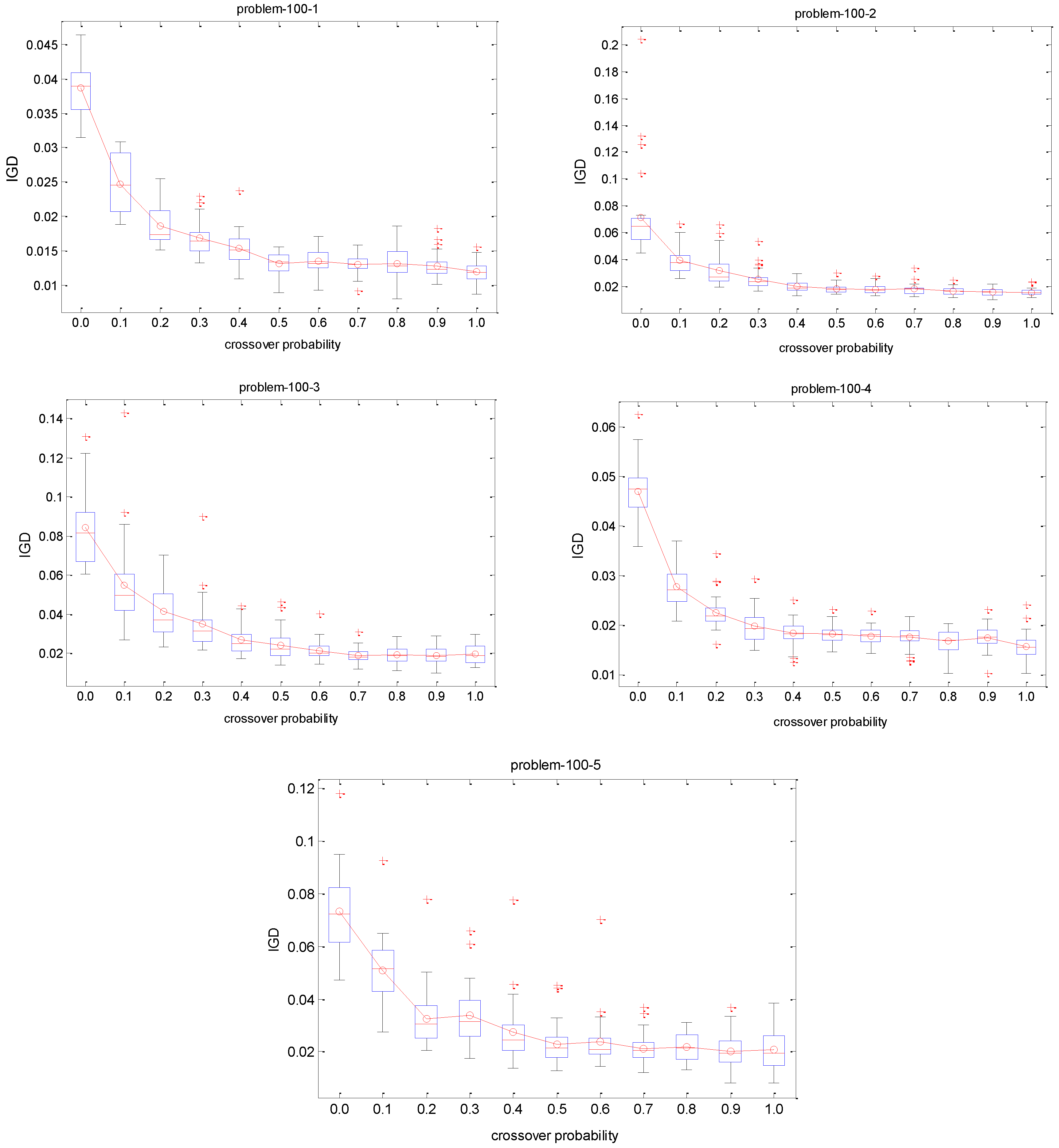
5.5.1. Selection of Crossover Probability
The crossover probability denoted by symbol
Pc, it is generated from 0 to 1.0 in increments of 0.1, and the mutation probability
Pm is 1/
n (
n is the number of jobs) in this experiment. The IGD metric is utilized to test the performance of the proposed algorithm for different
Pc on each instance since this IGD metric is a comprehensive indicator. We conduct 30 independent runs for each crossover rate on each test instance. The IGD trajectories against different
Pc are plotted in
Figure 8. The Y axis of each subfigure represents the IGD value and the X axis denotes the different
Pc. The red circle indicates the mean IGD value for a crossover rate combination. It can be observed that the IGD curves of small size problems with 10 jobs are stable with the increase of
Pc, which implies that the performance of the proposed algorithm is not sensitive to the
Pc. It is observed from
Figure 8 that the algorithm is more stable with the decreasing of the box’s length. In terms of descriptive statistics, a box plot is a convenient way of graphically depicting groups of numerical data through their quartiles. Box plots may have lines extending vertically from the boxes indicating variability outside the upper and lower quartiles, hence the terms box plot diagram. Outliers maybe plotted as individual points. Box plots are non-parametric: its display variation in samples of a statistical population without making any assumptions of the underlying statistical distribution. The spacing between the different parts of the box indicate the degree of dispersion (spread) and skewness in the data, and show outliers. In addition to the points of themselves, they allow one to visually estimate various L-estimators, notably the interquartile range, midhinge, range, mid-range, and trimean. Box plots can be drawn either horizontally or vertically. Concerning medium and large scale problems, the IGD value gradually decreases with the increase of
Pc. It means that crossover with a large probability can help to improve the performance of the proposed algorithm for coping with these scheduling problems. Therefore, the range (0.7, 1) for
Pc is recommended for decision makers when solving these scheduling instances.
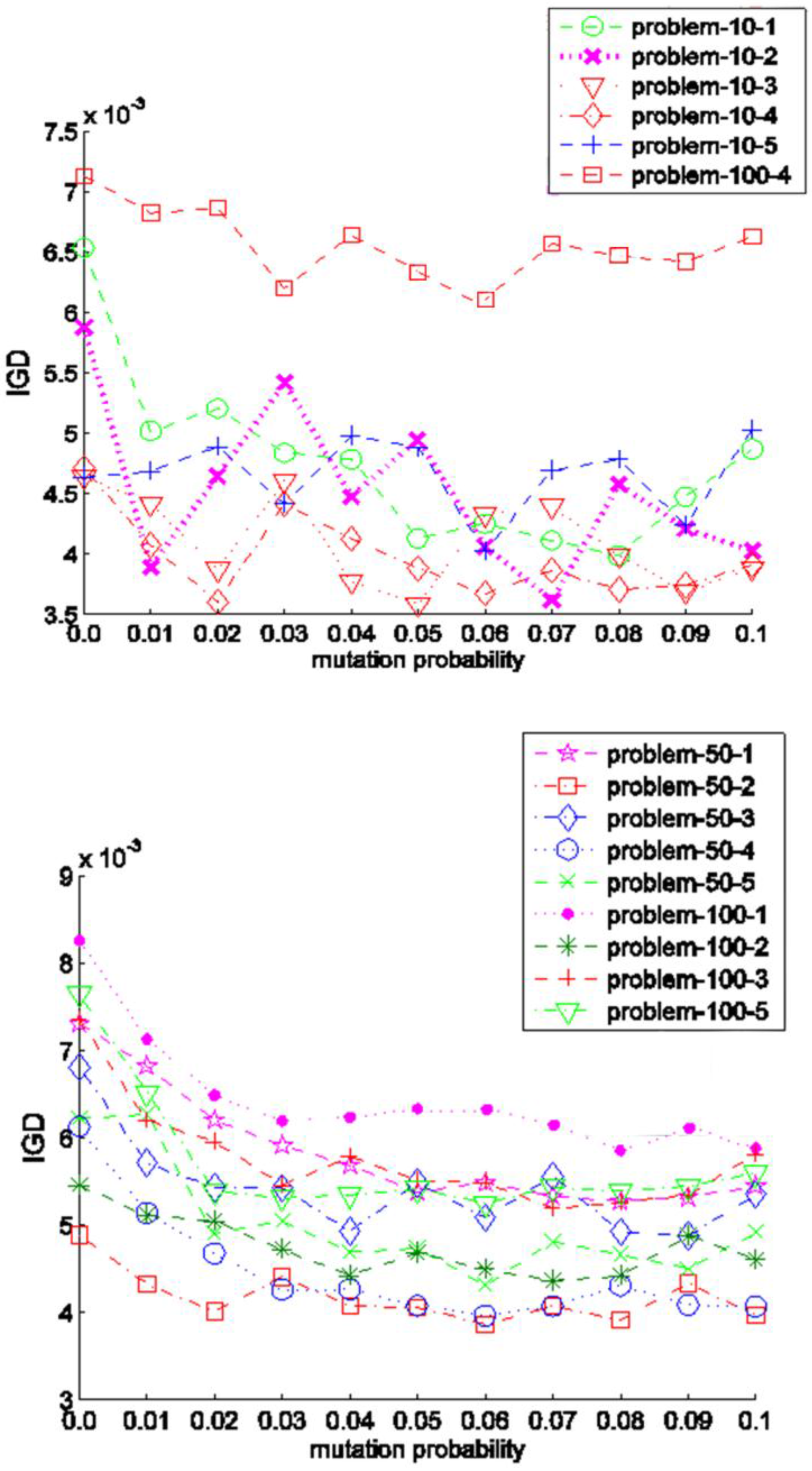
5.5.2. Selection of Mutation Probability
We further investigate these scheduling problems affected by mutation probability in this experiment. Here, crossover rate
Pc is fixed as 0.9 and mutation rate
Pm is updated from 0 to 0.1 with step of 0.01. We can run the same type of experiment to determine the optimal mutation probability. The mean IGD results are plotted in
Figure 9. The vertical axis of each subfigure denotes the IGD value and the horizontal axis represents the variation of
Pm. These scheduling problems can be divided into two categories. The first one is characterized as that a relatively stable IGD trend, indicating that the value of
Pm has little effect on the performance of the proposed algorithm. The instances with 10 jobs and problem_100_4 belong to this category. The second category, which consists of the rest medium and large instances except problem_100_4, is featured by a relatively high IGD value at the beginning, and then the IGD value decreases to a low level when
Pm is 0.04 and remains stable later. From the
Figure 9, the value 0.1 for
Pm is recommended.
In the following empirical studies, crossover and mutation probability in the proposed algorithm are set to 0.9 and 0.1, respectively.
5.6. Efficiency of Each Local Search Strategy
To prove the effectiveness of multiple local search strategies based on self-adaptive mechanism in LMOEA, we generate three variations of the LMOEA by adopting only one local search strategy and compare the behavior of each local strategy on the 15 problems. In this experiment, we use MOEA
S1 to denote LMOEA with only S1. Similarly, MOEA
S2 indicates LMOEA using only S2, and MOEA
S3 represents LMOEA with only S3.
Table 3,
Table 4 and
Table 5 show mean and standard deviation metrics on different algorithms in 30 independent runs.
From
Table 3,
Table 4 and
Table 5 it can be observed that MOEA
S3 obtains significantly better results on 9 out of 15 problems with comparison to MOEA
S1 and MOEA
S2 in terms of GD metric, while MOEA
S1 and MOEA
S2 can achieve the better GD values on two and four problems, respectively. Concerning Spread metric, the MOEA
S1 performs better than the MOEA
S2 and MOEA
S3 for most instances. However, MOEA
S2 is superior to MOEA
S1 and MOEA
S3 with regard to IGD metric. Therefore, it can be concluded that none of the three local strategies has a dominant performance for all instances.
When these three local search strategies are incorporated into our proposed LMOEA, we can observe that the proposed LMOEA wins the best IGD value on 11 out of 15 test instances. It means that the multiple strategies based on self-adaptive scheme can help to improve comprehensive performance (convergence and diversity). With regard to the GD metric, the LMOEA obtains the best value on 13 out of 15 test problems, which suggests our proposal can generate better PF toward PF* than the others with only single local strategy. That is to say, multiple local strategies based on self-adaptive scheme can enhance search efficiency since the candidate solution can select a proper local strategy to search optimal solutions. The proposed LMOEA with the multiple local search strategy is also superior to its three variations in terms of Spread metric.
Therefore, we can conclude that combination of these local search strategies can help to improve the search diversity and the selection of appropriate local operators can enhance the search efficiency. Besides, the results computed by the proposed LMOEA are more stable, which implies that the integration of multiple local search techniques based on self-adaptive mechanism can strengthen the robustness of the LMOEA.
5.7. LMOEA against Other MOEAs
To assess the performance of the proposed algorithm for scheduling problems, it is compared with other MOEAs such as NSGA-II, SPEA2, OMPSO, and MOEA/D in this section. First, the compared MOEAs are described as follows.
- (1)
NSGA-II is one of the most popular MOEA proposed by Deb et al. [
44]. The characteristic of NSGA-II is that it uses a fast non-dominated sorting and crowding distance estimation procedure. The fast non-dominated sorting technique is used to assign the parent and offspring population to different levels of non-dominated solution fronts. A crowding distance strategy is employed to maintain diversity of the population.
- (2)
SPEA2 was presented by Zitler et al. [
51]. In SPEA2 algorithm each individual has a fitness value which is the sum of its strength raw fitness and density estimation based on the distance to the
kth nearest neighbor. A new population is from the non-dominated solutions in both the original population and the external archive.
- (3)
OMOPSO is a multi-objective particle swarm optimization algorithm proposed by Sierra and Coello Coello [
52]. This proposal employs two external archives: one for storing the leaders for carrying out the flight and the other one for storing the final solutions. The crowding factor is used to remove the list of leaders whenever the external archive is full of final solutions. Only the leaders with the best crowding values are maintained. Additionally, the authors presented a scheme in which they divide the population into three different subpopulation.
- (4)
MOEA/D invented by Zhang and Hui. [
53] decomposes a multi-objective problem into a number of scalar sub-problems and optimizes them simultaneously. MOEA/D have received widely attention from evolutionary computation fields due to its fast convergence and good diversity.
To make a fair comparison in this experiment, the function evaluation number of all MOEAs is set to be 25,000 and all MOEAs use the same encoding scheme. Additionally, the initial population is randomly generated for the above MOEAs. The other parameters are shown in
Table 6. 30 independent runs are conducted for each algorithm on each test instance.
Table 7,
Table 8 and
Table 9 present the statistical results of the GD, Spread, and IGD metrics. From these tables, we can clearly observe that the proposed LMOEA outperforms its counterparts for solving these scheduling instances. Especially on the comprehensive metric IGD and convergence metric GD, the outperformances of the proposal are significant. More specifically,
Table 7 reveals that the proposed LMOEA is significantly better than the other four MOEAs for the GD metric on 8 out of 15 instances. SPEA2 can obtain better GD values for three instances, and MOEA/D and NSGA-II for two, respectively. It should be noted that OMOPSO fails to get better results on any one instance. We also observe from
Table 8 that LMOEA is superior to NSGA-II and OMOPSO for the Spread metric. In addition, LMOEA is competitive to SPEA2 and MOEA/D with regard to Spread metric. From
Table 9, LMOEA achieves significantly better results than the compared MOEAs in terms of the IGD metric. It should be pointed out that none of the MOEAs show a consistent and good behavior for all cases. However, compared with other MOEAs, the LMOEA is a very suitable tool for solving most instances since LMOEA shows a very good performance on this type of scheduling problems.
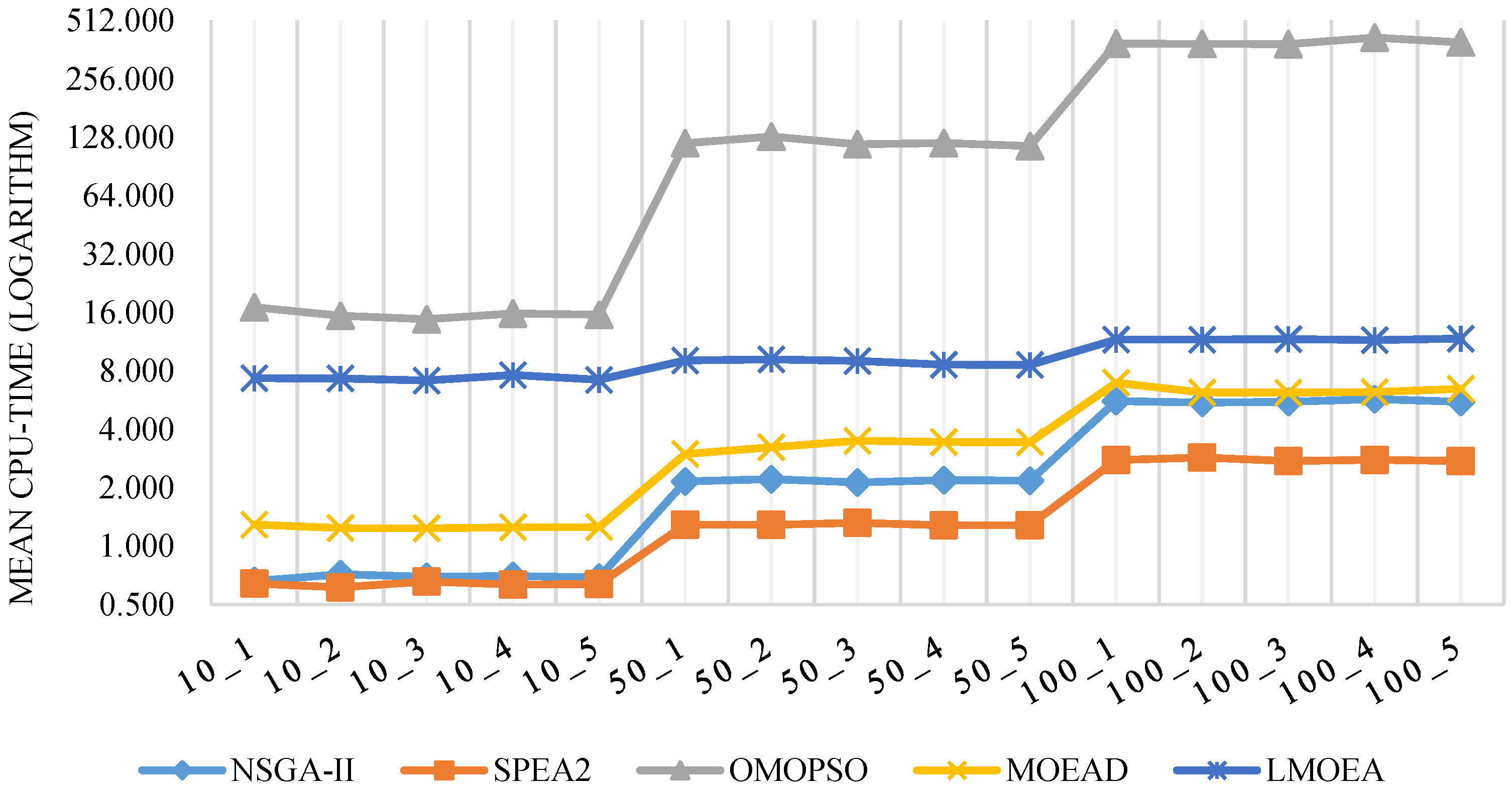
The average and standard deviation CPU-time of each algorithm has been reported in
Table 10, and the unit of time is second. In order to visualize the performance of five algorithms, the CPU-time costs on all test instances are selected for graphical representation for the
Figure 10, vertical axis taken logarithm. The figure illustrates and confirms some conclusions are derived from the numerical analysis with the performance criteria. It can be observed that SPEA2 is the fastest and OMOPSO is the slowest in solving all the problems. When there are more machines at each stage, CPU-time of each algorithm will be added accordingly, nevertheless LMOEA CPU-time also grows slower than other algorithms. The reason lies in the procedure of local search strategy construction. In this research, we present three different local search strategies (S1, S2 and S3) based on self-adaptive selection mechanism to obtain better approximate solutions, more details have been shown in
Section 4.2.4. Consequently, LMOEA can benefit from a local search strategy which aims at enhancing exploitation ability of the algorithm. In contrast, OMOPSO does not include any heuristic information for reducing running time.
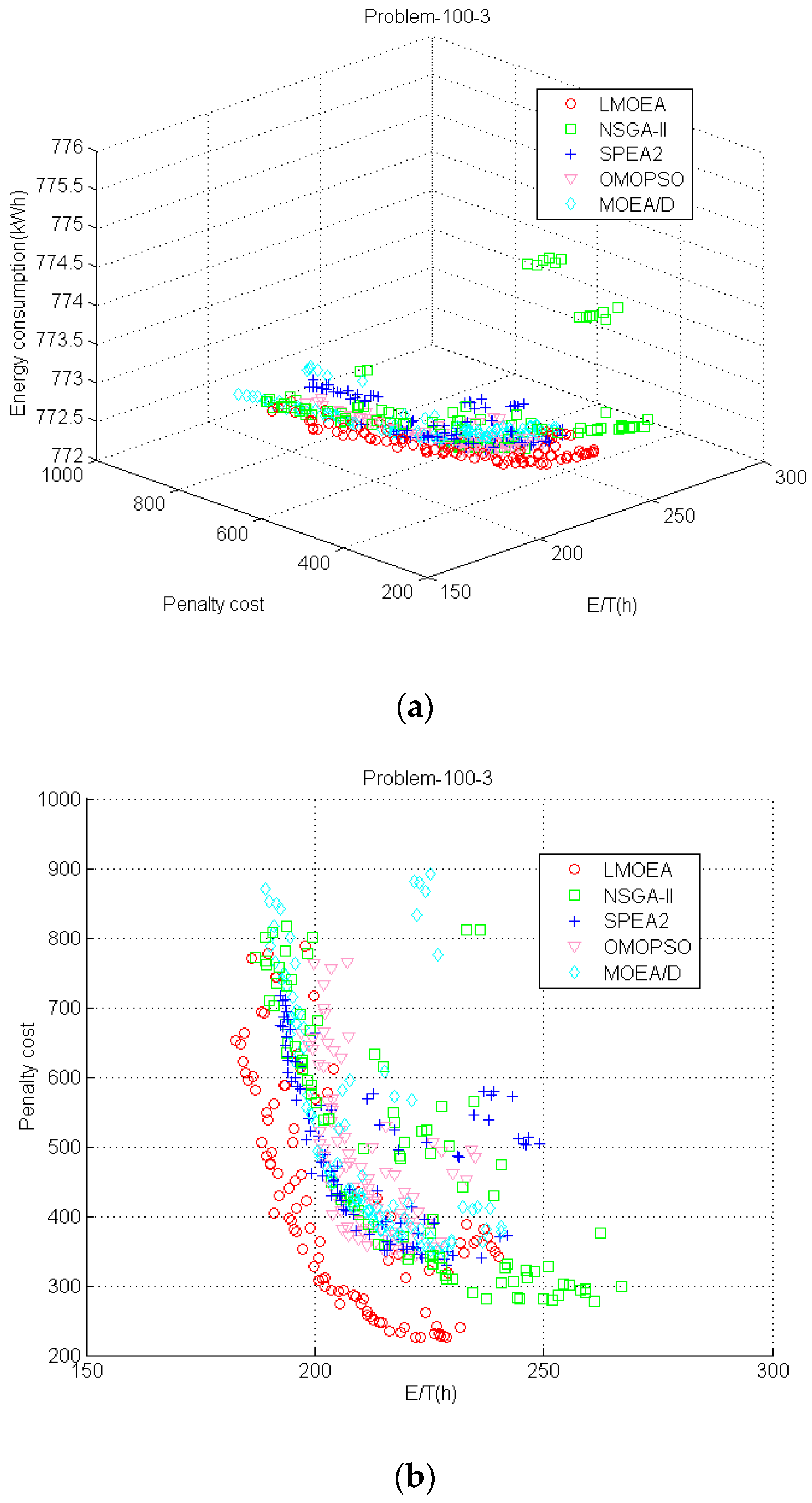
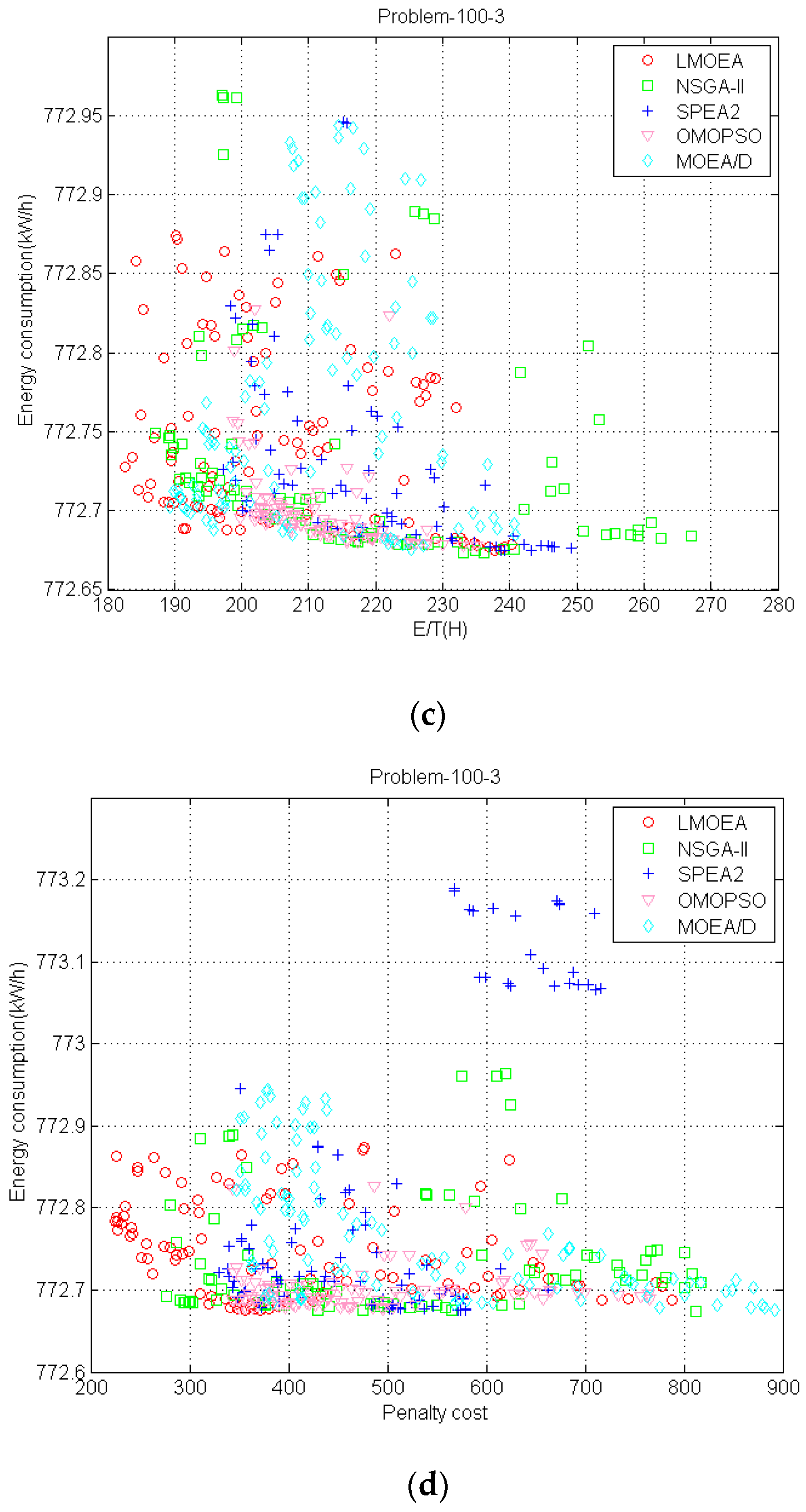
To give a graphical overview of the performance of these algorithms,
Figure 11 shows the
PF approximations obtained by different MOEAs in the run with the best IGD value for the problem_100_3 from different perspectives. In all the figures, the total E/T represents
f1 objective; penalty cost represents
f2 and the total energy consumption denotes
f3.
Figure 11a presents
PF in 3D space and it is hard to judge which MOEA is the best one among them. However, it is evident from
Figure 11b that the proposed LMOEA reaches better approximations toward
PF* than the other MOEAs in 2D space, which denotes the LMOEA has good convergence performance. It also indicates the two objectives of the total E/T and cost are conflicted with each other. As shown in
Figure 11c,d, even though the SPEA2, OMOPSO and LMOEA can approach closer toward
PF* than NSGA-II and MOEA/D, the proposed LMOEA can cover a wider range than SPEA2 and OMOPSO. It implies that
PF obtained by LMOEA has good diversity. SPEA2 also covers a large area, but it tends to converge to local areas. The outperformance of LMOEA can be attributed to multiple local search strategies based upon adaptive mechanism, by which LMOEA can search preferable solutions in its neighborhood.
According to the results in the above experimental studies, the LMOEA is a promising approach to cope with this kind of scheduling. Additionally, several observations are also drawn.
- (1)
Different crossover operators have different impacts on the performance of the proposed LMOEA. The SBX operator is the best choice among the compared crossovers in LMOEA for solving the scheduling instances.
- (2)
Compared with the adoption of only one local search strategy, integration of multiple local search techniques with self-adaptive mechanism can significantly improve the behavior of the LMOEA.
- (3)
The objectives of total E/T, penalty cost and energy consumption are in conflict with each other according to
Figure 11.
- (4)
The proposed LMOEA can perform better than its rivals such as NSGA-II, OMOPSO, SPEA2, and MOEA/D for most scheduling instances.
6. Case Study
Consider the following single machine scheduling problem with controllable processing and setup times from a realistic welding workshop in Henan Weihua Heavy Machinery Co., Ltd, Changyuan, China. This welding shop is required to process 12 types of jobs that should be passed through only one machine. The relative data including Machine power, available machines, job number, processing times, setup times is provided in
Table 11,
Table 12,
Table 13 and
Table 14.
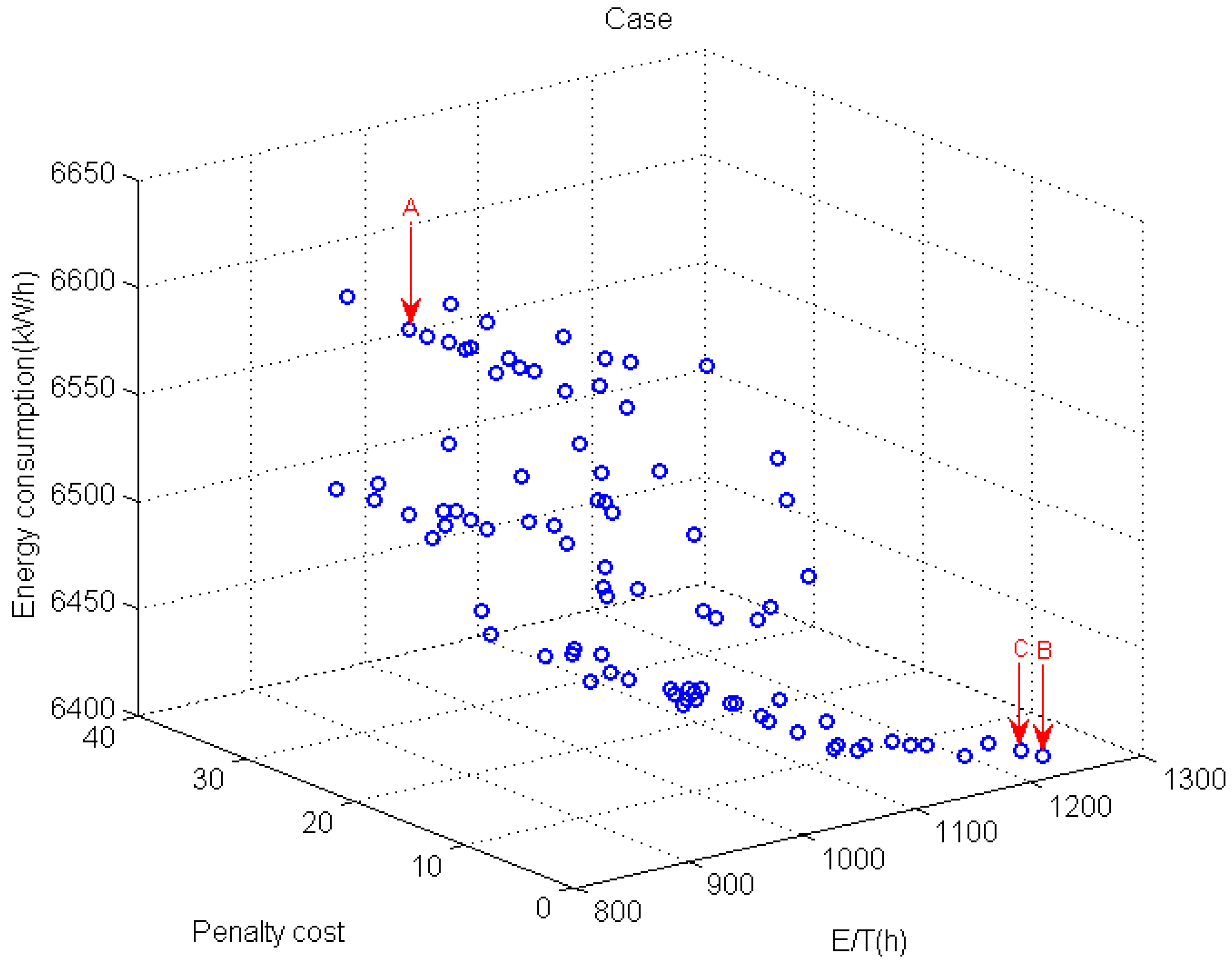
The Pareto front obtained by the proposed LMOEA is presented in
Figure 12. It is obviously observed that the proposed LMOEA is capable of providing high quality and good diversity solutions. Point A, B and C represent three extreme objective values, respectively. These points can be expressed as follows: A (813.8, 16.5, 6625.6), B (850.8, 0, 6639), and C (1213.60, 0, 6411). The above extreme objectives correspond to the following three non-dominated solutions.
Solution at point A: π = {J5, J11, J1, J2, J3, J6, J12, J7, J10, J9, J8, J4}, m= (0, 0, 0, 0, −3, 0, −3, 0, 0, 0, 0, 1,)
Solution at point B: π = {J5, J11, J1, J2, J6, J12, J3, J4, J10, J7, J9, J8}, m= (0, 0, 0, 0, 0, 0, 0, 0, 0, 0, 0, 0,)
Solution at point C: π = {J4, J7, J2, J1, J3, J6, J12, J8, J5, J10, J11, J9} m= (0, 0, 0, −1, 0, 0, 0, 0, 0, 0, 0, 0,)
The computed results indicate that the proposed Energy-efficient scheduling problems model and corresponding local MOEA can indeed optimize the decision target, effectively solving the process-based problem. However, it is not possible to obtain a dispatch plan that simultaneously optimizes the penalty cost, total process energy consumption and E/T because optimizing one indicator inevitably worsens the others.
7. Conclusions
This paper developed a multi-objective mathematical model considering both productivity (i.e., E/T and cost) and energy consumption on a single machine environment. In this new model, controllable processing times are employed to approach toward JIT production, and the energy consumption can be reduced by operational and the turn off/on method. The proposed algorithm LMOEA is utilized to solve this scheduling problem. This algorithm LMOEA is different from other MOEAs where three different local search strategy based on adaptive scheme is to improve search performance of the algorithm. There are still some limitations. Firstly, the heuristic information based on problem property has not been introduced into the LMOEA. Secondly, the proposed algorithm contains some parameters, which affect the performance of the algorithm.
Experimental studies are conducted to measure the performance of the proposed LMOEA algorithm for scheduling instances. First, a SBX operator is chosen as an appropriate crossover operator in the LMOEA by comparing different crossovers on all instances, and then the impact of the crossover and mutation probability is also analyzed. Finally, the computational experiments demonstrate that the proposed LMOEA outperforms its rivals such as NSGA-II, SPEA2, OMOPSO, and MOEA/D for most scheduling problems. In addition, the main contributions of this work are as follows:
- (1)
A multi-objective scheduling model, which considers three objectives, is constructed. A hybrid MOEA with multiple local search strategy is developed to effectively solve this kind of the scheduling.
- (2)
A new solution representation is provided for this kind of the scheduling. It also offers a new idea in solving scheduling problems.
- (3)
In this work, the mutation operator composed of two types of mutation techniques is proposed. The first mutation technique can adjust amount of compression of job processing times. The second mutation technique can exchange order of jobs. It implies the mutation operator can helps the algorithm to escape from local optimum.
- (4)
According to the above parametric experiment, both parameters Pc and Pm have critical effect on the performance of the LMOEA for most instances. The range (0.7, 1) for Pc and 0.1 for Pm are recommended for decision makers when solving these scheduling instances.
- (5)
Multiple local strategies based on adaptive selection scheme can improve the performance of the LMOEA on instances.
With respect to future work, the proposed algorithm should be evaluated on different scheduling environments such as job and open shop scheduling environment to validate its more general applicability. Another issue for future research is to improve the search efficiency of the algorithm by incorporating current new techniques such as deep learning. In addition, operation speed associated with processing times will be considered in future research.


