Bidirectional Incentive Model for Bicycle Redistribution of a Bicycle Sharing System during Rush Hour

Abstract

Redistribution is an important part of operational activities in a bicycle sharing system (BSS). This paper proposes that there are two types of users in a BSS: leisure travelers and commuters. The operators and the government are adopting the bidirectional incentive model (BIM) to improve their service level of redistribution. That is, the BIM stimulates leisure travelers to actively respond to bicycle resetting needs of the system; on the other hand, it guides commuters by encouraging them to avoid travelling in peak periods. This is beneficial to achieve the goals of reducing the scheduling pressure on bicycles during rush hour, and even to realize the self-resetting of the BSS. In this paper, we explore three scenarios for implementing BIM through cooperation between the operator and the government. By exploiting Stackelberg games in all models, we illustrate the quantity of users in three different travel behaviors, and surplus value of these users respectively. We also consider the trend of the profit of the operator and the government when some changes of parameters are made. The numerical analysis and case discussion find that the strategy of the operator implementing BIM with a subsidy is the best method for developed regions. In a developing region, the strategy of implementing the BIM with a direct government subsidy to users is the best choice in a small or tourist city. In these cities, the proportion of leisure travelers is always larger than 50%, resulting in a significant incentive effect. The strategy of the operator implementing BIM without a subsidy is the best choice for the large and medium-sized city.

1. Introduction

Nordic countries spearheaded bicycle sharing systems and this green, economical, flexible, sustainable mobility model has garnered interest worldwide [1]. By the end of 2015, over 1000 cities participated in BSS [2], and a BSS provides an individual increased flexibility to access a bicycle without burdens of using traditional transport action methods (such as usage time limitation and inconvenience caused by traffic congestion) [3]. People can use the public bicycle to commute and they can easily reach their destinations. With the development of the BSS, many operational aspects are now being scrutinized. Lihong et al. showed that a bicycle sharing system was a product service system. One of the most difficult operational tasks is to strike a balance between the provision of services and its physical design [4]. Dell et al. indicated that the major problem concerning the operator in a BSS is to redistribute bicycles quickly during rush hour [5]. If the operator cannot avoid the system imbalance (it is hard to park at some stations, while other stations have no bicycles available to rent), the satisfaction of users declines and users may even abandon this new mode of transport action [6,7].

Therefore, researchers are paying closer attention to the ways to meet the fluctuating demands of users. Most previous studies were focused on two aspects: the optimized model of the location of bicycle stations and the optimal design of bicycles scheduling for reposition. As for optimizing the location of bicycle stations to satisfy the potential demand, García-Palomares et al. proposed a GIS-based method with location-allocation models [8]. They tested two solutions in location-allocation models and proved that the maximize-coverage solution performed better in terms of efficiency, since it maximized the potential demand covered by the stations. Martinez et al. used a Mixed Integer Linear Program to optimize the location of stations and the relocation of bicycles in Lisbon’s BBS [9]. They provided a better way to operate these complicated systems. For dealing with the repositioning problem, Forma et al. proposed a three-step mathematical programming-based heuristic for the static bicycle repositioning problem [10]. This method was tested on instances of the Vélib system (in Paris), and the result showed that it was suitable for large, real-life instances of the problem. DiGaspero et al. incorporated the two constraint programming models in a large neighborhood search approach to tackle the problem of balancing bicycle sharing system (BBSS) [11]. They showed that their approach was more competitive than other existing approaches for BSS implementation in real life. Alvarez-Valdes et al. proposed a procedure to solve the problem of BBSS [12]. This procedure provided operational strategies with redistribution algorithms by estimating the unsatisfied demand on available bicycles or lockers at each station. This procedure had been tested for its usefulness as a planning tool in the BBS in Palma de Mallorca (Spain). Vogel et al. proposed a service network design-relocation services (SND-RS) approach to cover the issues of BBSS [13]. However, SND-RS neglected the information about empty trips of vehicles, in order to make a stronger anticipation of operational decisions. Based on this, Neumann-Saavedra et al. added the concept of service tours (ST) to extend the SND-RS to a new service network design approach called service network design-service tours (SND-ST). Here, ST is somehow an abstraction of the vehicle fleet meaning that a capacitated vehicle is assigned to each ST when implemented in the operational planning level [14].

The existing studies mainly focus on optimizing the repositioning of bicycles, by deploying a fleet of trucks to redistribute bicycles among stations based on estimating the demand of users. Although the efficiency of resetting can be improved by optimizing the scheduling route of bicycles, there are associated costs and carbon emissions caused by trucks scheduling, and the performance of scheduling is also affected by the congestion of vehicles during the peak period. Therefore, the above-mentioned methods have certain limitations. To overcome these limitations, is there a way to convert the operator from passively respondence to actively lead users’ travel demands? In other words, is it possible for the operator to encourage the users by themselves to solve the imbalance problem in the BSS? Singla et al. attempted to use a crowdsourcing mechanism with monetary reward aiming at changing bicycle users’ travel behavior in accordance with the bicycle repositioning requirement [15]. They designed the first dynamic incentive system for bicycle redistribution and deployed it through a smart phone application in a real BSS. Moreover, the ‘surge’ policy in rush hour is commonly used by operators of different public transportations to balance traffic pressure in congested cities, such as Singapore, London and Beijing [16].

Researchers have pointed out that price discrimination was an effective means of regulation in the development of many traditional transport systems, and the effect of price discrimination tended to intensify over time [17,18]. Therefore, research regarding dynamic pricing of public transportation attracts researchers attention increasingly [19]. Stavins et al. found that the performance of price discrimination would be affected by ticket restrictions; and the performance will improve when the airline markets become more competitive [20]. Woo et al. used a generalized Leontief demand system to investigate the effects of a ‘tunnel congestion’ toll adjustment policy in Hong Kong, and concluded that changes in tolls could cause shifts in the transportation demand [21]. Daganzo et al. proposed a quasi-optimum formula for the usage-based, time-dependent congestion toll, and found that the proposed method delivered greater user benefits than trip-based tolls (trip-based tolls indicates a charge based on trip length) [22]. Jiang et al. focused on optimal airport pricing; they proposed a model that integrated with terminal and runway congestion, and found that, when the business passengers have higher relative schedule-delay costs, and business passengers were charged higher than leisure passengers, it could yield the first-best outcome; however, the uniform airfare does not yield the best result [23]. Tan et al. investigated dynamic congestion pricing schemes to minimize cost and time of a tolled transportation network. These schemes considered route adjustment behavior of travelers and their heterogeneity on value of time (VOT). They proposed a toll updating scheme by using the implicit Runge-Kutta method [24]. Zangui et al. provided a path toll to substantially reduce the charge burden of motorists, which is more flexible than link tolls [25].

From the above literature we find that, no matter what type of transportation is considered, in order to use the price incentive mechanism to relieve rush hour traffic pressure by operators, and ensure their profits are not affected, the prerequisite is for the users to have heterogeneity in degrees of PS and VOT. This makes it possible to achieve traffic diversion through utilizing price differentiation by guiding the different types of users to choose different transportation modes. As we know, the users of a BSS can be divided into two categories with heterogeneity, such as commuters and leisure travelers. Therefore, it makes sense to apply the price incentive mechanism to relieve the pressure of BSS resetting, and some efforts have been made to do so. Ruch et al. proved that dynamic pricing could control the travel behavior of users by employing an Agent-Based Model with parameters consisting of real historical data [26]. They proved that simple proportional price control rules can enhance the service level without relying on the bicycle redistribution staff to balance the “one-way” phenomenon. Aeschbach et al. proved that a BBS could be balanced through user cooperation [27]. In other words, this balance was achieved by sending “control signals” for bicycle users to change their intended travel plans via a mobile application. The simulated results showed that the service level of the system increases as the proportion of cooperating customers grows. Based on the above literature, it is obvious that price adjustment is a powerful method to solve congestion through encouraging users to change their routes [28]. With the development of mobile Internet, sending real-time control information to the users and collecting fees dynamically have become possible. Moreover, a BSS is generally supported by governments as a public project. Government subsidy is the main income for many of BSS [29]. Therefore, the government subsidy should be taken into consideration.

Motivated by the above research, we propose a bidirectional incentive model (BIM). The key point of BIM is illustrated as follows: Users who rent or return bicycles from the stations which have only a small number of bicycles or locks are charged extra money. Meanwhile, users who cooperate with the operator in relocating bicycles are rewarded. In this paper, we discuss three models to study the implementation of BIM with Stackelberg game theory in different subsidy strategy scenarios. We found that these three scenarios presented here were optimal under different conditions.

The rest of the paper is organized as follows. We present three Stackelberg game model descriptions under different scenarios in Section 2. Section 3 shows the optimal decisions of the operator and the government. We analyze the impact of some parameters on these models in Section 4. A case discussion is undertaken in Section 5. The last section is the conclusion.

2. Model Description

It is an interesting phenomenon that many supermarket operators successfully utilize shopping cart trolley coin locks to impel customers to return the shopping cart to a specified destination. When the customers want to use a cart, they must put a coin into the cart lock. When they return the cart to the specified place, the coin is returned to them. If someone leaves the shopping cart at some random spot (has higher VOT) without taking the coin back (who has lower PS), there must be someone (who has a higher PS and lower VOT) who returns the shopping cart in order to obtain the coin. Similarly, supervisors of the BSS also hope that users could return bicycles to the specified place. There are two types of users in a BSS with different PS and VOT: commuters and leisure travelers. Inspired by the phenomenon mentioned above, this paper proposes a bidirectional incentive model to guide users changing their travel behaviors. The bidirectional incentive is different from the one-way incentive (such as, some regions charges congestion fees from travelers who travel in the peak flow direction). In the bidirectional incentive, users are charged in the BSS who travel in the peak flow direction, and users who travel in the inverse peak flow direction are rewarded. That is the reason it is called “bidirectional”.

In this paper, we study a two-echelon bicycle sharing system consisting of an operator and a government. By implementing the BIM, the interactive process among the government, the operator and users is as follows: Firstly, the operator must determine the quota of charge or reward, and the government must determine the amount of subsidy. Secondly, travel behaviors of users could yield the best to their advantages. Lastly, the operator and the government meet the incentive commitments according to different behavioral choices of users. In this paper, we analyze three scenarios based on different strategies of implementing the BIM. Furthermore, we compare these strategies with their applicable conditions, advantages, and disadvantages. 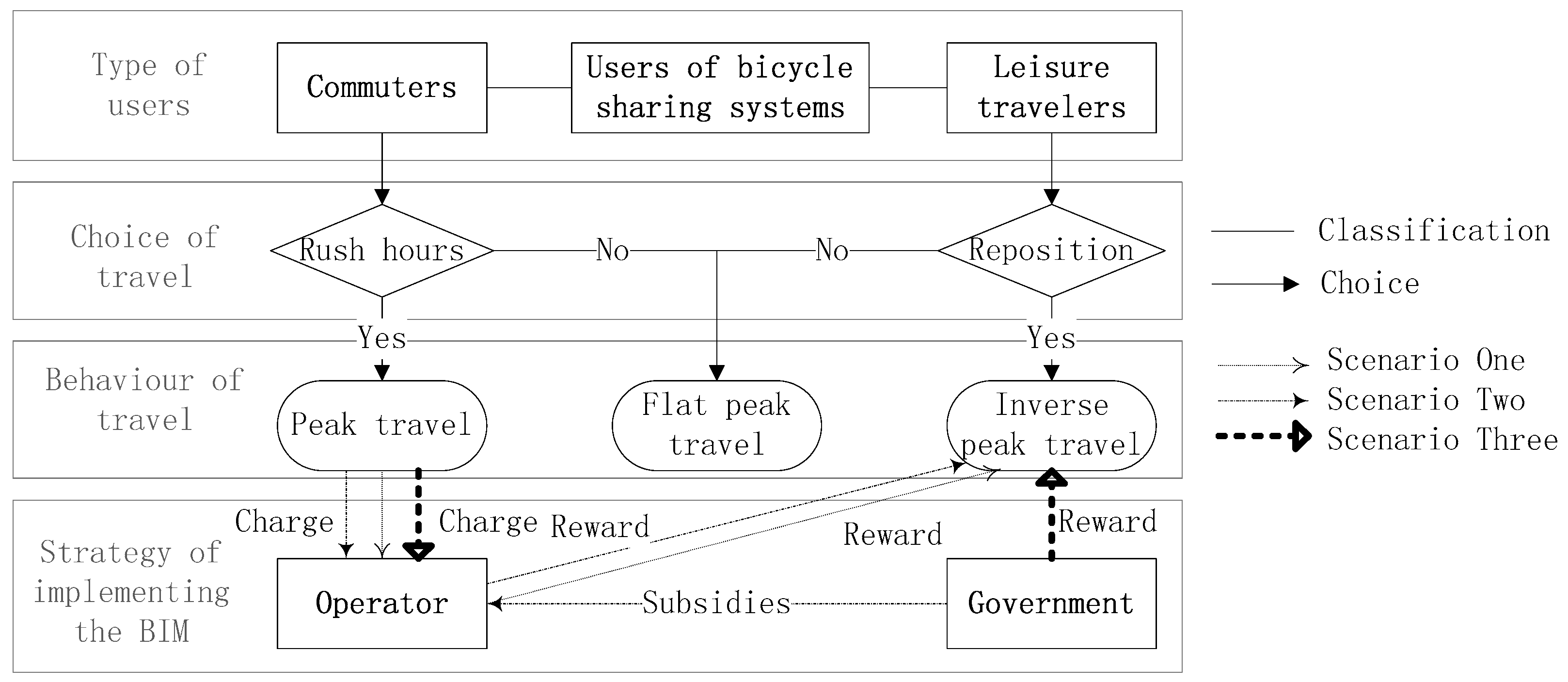Figure 1 illustrates the framework of our models.

For clarification purpose, we use PT to stand for peak travel, which refers to the travel behavior which borrows bicycles from stations without many available bicycles, and returns bicycles to stations without many locks. Commuters always travel in this way. We use IPT to stand for inverse peak travel, which refers to the travel behavior which helps resetting bicycles in the BSS. Leisure travelers are encouraged to exhibit the travel behavior of IPT. We use FPT to stand for flat peak travel, which refers to two types of travel behavior, one is to travel during off-peak hours; and the other one is to travel during the peak hour with some special condition. This condition means that at most one station is the frequently used station, either the initiating station or arrival station.

The description of Figure 1 is as follows:

(1)

Types of users. According to the purpose of travel, there are two types of users in the BSS: the commuter and the leisure travel. Before implementing the BIM, the former always exhibits the behavior of PT before, and the latter always exhibits the behavior of FPT. The main travel purpose of the commuter is going to work. The travel purposes of the leisure traveler are more diverse, such as exercising, travelling and sightseeing, daily shopping and so on.

(2)

Choice of travel. After implementing the BIM, if the commuter chooses to travel at peak hour, their behavior of travel conforms with PT, otherwise FPT. For leisure travelers, if they choose to help reset bicycles, their travel behavior conforms with IPT, otherwise FPT.

(3)

Behavior of travel. In order to quantify the effect of implementing BIM, the travel behavior of users is divided into three types: IPT, PT and FPT. The evaluation of implementation effect is mainly based on the conversion among IPT, PT and FPT.

(4)

Strategy of implementing the BIM. Based on different strategies of implementing the BIM, there are three scenarios. In scenario one, we discuss the case that the operator implements the BIM without subsidy. In scenario two, we discuss the case that the operator implements the BIM with subsidy. In scenario three, we discuss the case that the government directly rewards users who choose to exhibit the travel behavior of IPT. It should be noted that, in these three strategies, both the operator and the government neither reward nor penalize the users who exhibit the behavior of FPT.

For the sake of convenience, the following notations in

Table 1. Notation list.

Notation	Definition
$p$	Unit price of the user who exhibit the behavior of PT $p\ge 0$.
$B$	Unit subsidy of the user who exhibit the behavior of IPT $B\ge 0$.
${\theta }_1,{\theta }_2,{\theta }_3$	The ratio of the unit subsidy to the unit price in scenario one, scenario two, and scenario three, respectively.
$c$	Unit cost of redistributing one bicycle by truck $c\ge 0$.
$S$	Unit subsidy that the government provides to the operator, $S\ge 0$.
$b_1,b_2$	The degree of price sensitivity of the commuter and the leisure traveler, respectively.
$\alpha$	The ratio of the degree of price sensitivity of the leisure traveler to the commuter; that is $\frac{b_2}{b_1}$.
$q_1,q_2$	The quantity of users in the type of commuters and leisure travelers in the BSS, respectively.
$\beta$	The ratio of quantity of users in the type of leisure travelers to that of commuters in the BSS, that is $\frac{q_2}{q_1}$.
$\mu$	The marginal cost of public finance capital, $1\le \mu \le 1.5$ [30]
$Q_g,Q_p,Q_n$	The quantity of users who exhibit behaviors of PT, FPT, and IPT, respectively.$Q_g\ge 0,Q_p\ge 0,Q_n\ge 0$
$D_g,D_p,D_n$	The surplus value of users who exhibit behaviors of PT, FPT, and IPT, respectively.$D_g\ge 0,D_p\ge 0,D_n\ge 0$
$D_1,D_2,D_3$	The sum of the surplus value of all users during rush hour in scenario one, scenario two, and scenario three, respectively. $D_i=D_g+D_p+D_n,(i=1,2,3)$
${\pi }_1,{\pi }_2,{\pi }_3$	The profit of the operator during rush hour in scenario one, scenario two and scenario three, respectively.
$U_1,U_2,U_3$	The profit of the government during rush hour in scenario one, scenario two, and scenario three, respectively.

are the major variables and parameters used throughout this paper.

We simplify some complex conditions under the stipulation. The simplification does not change the essence of the problem and the following assumptions are made for each model:

Assumption 1:

In this paper, we consider only one operator and one government in a BSS;

Assumption 2:

The proposed model focuses on the rebalance in BSS during rush hour, so it only discusses the new changes of stakeholders’ profit after implementing the BIM. It does not consider the income from the basic fee and other operational cost;

Assumption 3:

The quantity of users who exhibit the travel behavior of PT must be larger than IPT; that is $Q_g\ge Q_n$. If $Q_g\le Q_n$, the BSS has no need to reset bicycles and the BIM is pointless;

Assumption 4:

In this paper, we assume that commuters would not exhibit the travel behavior of IPT, but it is possible for them to choose the behavior of FPT in order to avoid being charged. The leisure travelers would not exhibit the travel behavior of PT, but it is possible for them to choose the behavior of IPT in order to obtain the reward;

Assumption 5:

The subsidy from the government is always sufficient to meet the requirement of profit maximization;

Assumption 6:

The BSS is a public transport project; so the government has responsibility to guide the operator of this BSS to provide excellent service and charge a relatively low fee from users. Through government support and supervision, the BSS could develop sustainably. Therefore, in this paper, we assume the government has a leading position in the BSS, and the operator is a follower. The operator will adjust its operational strategy according to government decisions.

3. Optimal Strategies in Different Scenarios

In order to explore the effect of implementing BIM in the BSS during rush hour, and find out the best condition and strategy for BSS profit maximization, this section studies the performance of a BSS in three different scenarios: the implementation of BIM by the operator without government subsidy (Scenario One), the implementation of BIM by the operator with government subsidy (Scenario Two), and the implementation of BIM by the cooperation of the government and the operator (Scenario Three). In scenario three, the government is responsible for giving rewards to users who exhibit the behavior of IPT, and the operator is responsible for charging fees from users who exhibit the behavior of PT.

Formulas which describe the quantity and surplus value of the users in different travel behaviors will be used in all scenarios. The quantity of users in the behavior of PT, IPT and FPT can be expressed as follows, respectively:

$$Q_g=q_1-b_{1}p$$

(1)

$$Q_n=b_{2}B$$

(2)

$$Q_p=q_2-b_{2}B+b_{1}p$$

(3)

Equation (1) expresses the quantity of users who exhibit the behavior of PT will be reduced by $b_{1}p$. Equation (2) expresses the quantity of users who exhibit the behavior of IPT will be increased by $b_{2}B$. Equation (3) expresses the quantity of users who exhibit the behavior of FPT will be reduced by the users who turned into IPT (that is $b_{2}B$). This quantity will be increased by the users who turned into PT (that is $b_{1}p$).

The surplus value of users who exhibit the behavior of PT, IPT, and FPT can be expressed as follows, respectively:

$$D_g=\frac{1}{2}p\left[2q_1-b_{1}p\right]$$

(4)

$$D_n=\frac{1}{2}{b}_2{B}^2$$

(5)

$$D_p=\frac{1}{2}B(q_2-b_{2}B)+\frac{1}{2}{b}_1{p}^2$$

(6)

According to the theory of consumer surplus from the welfare economics, the surplus value of the users in the BSS can be measured by the area below the demand of the travel curve and above the price/reward line. For further details and logics of Equations (1)–(6) employed in this article, please see the analysis of Willig [31].

Two constraints are shown below for the model matchness with reality:

$$Q_g-Q_n\ge 0\stackrel{Deformation}{\to }\theta \le \frac{q_1-b_{1}p}{\alpha b_{1}p}$$

(7)

$$Q_p\ge 0\stackrel{Deformation}{\to }\theta \le \frac{\beta q_1+b_{1}p}{\alpha b_{1}p}$$

(8)

Equation (7) expresses that the quantity of users who choose the behavior of IPT must be less than or equal to that of users who choose the behavior of PT. Equation (8) expresses that the quantity of users who choose the behavior of FPT cannot be less than zero. To simplify the analysis, we combine these two constraints into one constraint. The merged constraint can be expressed as follows:

$$s.t.\{\begin{array}{c}\beta \le 1-\frac{2b_{1}p}{q_1}\begin{array}{cc},& s.t.\theta \le \frac{\beta q_1+b_{1}p}{b_1\alpha p}\end{array}\\ \beta \ge 1-\frac{2b_{1}p}{q_1}\begin{array}{cc},& s.t.\theta \le \frac{q_1-b_{1}p}{b_1\alpha p}\end{array}\end{array}$$

(9)

Equation (9) expresses that, when $\beta \le 1-\frac{2b_{1}p}{q_1}$, the constraint of the model is $\theta \le \frac{\beta q_1+b_{1}p}{b_1\alpha p}$; when $\beta \ge 1-\frac{2b_{1}p}{q_1}$, the constraint of the model is $\theta \le \frac{q_1-b_{1}p}{b_1\alpha p}$. In this paper, we assume that $b_1,p$, and $q_1$ are constant. Therefore, $1-\frac{2b_{1}p}{q_1}$ in Equation (9) is a constant as well.

3.1. Scenario One: The Implementation of BIM by the Operator without Subsidy

In this scenario, the operator implements the BIM spontaneously, or is enforced to implement the BIM by mandatory provisions of government. Thus, there is no subsidy from the government. The operator charges fees from the users who exhibit the behavior of PT, and uses them to compensate users who exhibit the behavior of IPT. This is a Stackelberg game led by the government. We solve the gaming process for the subgame-perfect equilibrium by using backward induction. Hence, operator’s objective function is as follows:

$$\max {\pi }_1=p{Q}_g-B{Q}_n-c(Q_g-Q_n)$$

(10)

where the first term on the right hand side (RHS) expresses the income of the operator by charging extra fees from the users who exhibit the behavior of PT. The second term expresses the reward to the users who exhibit the behavior of IPT. The last term expresses the cost of rebalancing bicycles by the operator during rush hour. The crux of the operator here is to choose a suitable value of ${\theta }_1$ to maximize its profit. Differentiating the profit function ${\pi }_1$ with respect to ${\theta }_1$ yields:

$$\frac{\partial {\pi }_1}{\partial {\theta }_1}=\alpha {\mathrm{b}}_{1}p(c-2p{\theta }_1)$$

(11)

where $\frac{{\partial }^2{\pi }_1}{\partial {\theta }_1{}^2}=-2\alpha {\mathrm{b}}_1{p}^2<0$ to ensure the concavity of the function ${\pi }_1$, then we let $\frac{\partial {\pi }_1}{\partial {\theta }_1}=0$ in Equation (11), which generates the optimal rate ${\theta }_1^{*}$ of the operator:

$${\theta }_1^{*}=\frac{c}{2p}$$

(12)

Both the operator and the government need to satisfy the constraint of Equation (9), and the detailed analysis is shown in Appendix A.

Then, the best response function ${\theta }_1$ of the operator is substituted in the objective function of the government, which is shown as follows:

$$\max U_1={\pi }_1+D_1=2{\mathrm{pq}}_1+b_{1}p(c-1)-\frac{1}{2}\alpha b_1{p}^2{\theta }_1({\theta }_1+\beta )-c{\mathrm{q}}_1+\frac{1}{2}{\theta }_{1}p\beta q_1+c\alpha b_1{\theta }_{1}p$$

(13)

where the first term on the right hand side (RHS) expresses the gross profit realized by the operator. The second term expresses the sum of users’ surplus value. We can use the optimal ${\theta }_1$ to calculate the value of ${\pi }_1,U_1$.

3.2. Scenario Two: The Implementation of BIM by the Operator with Subsidy

To carrying out the BIM without any support, the operator may not have motivation to promote the change if he would not receive a sufficient return in some cases. At this time, the support from the government becomes very crucial. In this scenario, the government gives a corresponding subsidy to the operator, according to the performance of implementing the BIM. The solution procedure is the same as Section 3.1. The objective function of the operator is as follows:

$$\max {\pi }_2=p{Q}_g-B{Q}_n-c(Q_g-Q_n)+S{Q}_n$$

(14)

where the first three terms of RHS expresses the income of the operator, and the last term expresses the subsidy income. For $Q_n$ can reflect the effect of implementing the BIM, the total amount of subsidy is positively correlated with $Q_n$. The crux of the operator here is to choose a suitable value of ${\theta }_2$ to maximize its profit. Differentiating the profit function ${\pi }_2$ with respect to ${\theta }_2$ yields:

$$\frac{\partial {\pi }_2}{\partial {\theta }_2}=\alpha {\mathrm{b}}_{1}p(c+S-2p{\theta }_1)$$

(15)

where $\frac{{\partial }^2{\pi }_2}{\partial {\theta }_2{}^2}=-2\alpha {\mathrm{b}}_1{p}^2<0$ is ensure the concavity of the function ${\pi }_2$, then we let $\frac{\partial {\pi }_2}{\partial {\theta }_2}=0$ in Equation (14), which generates the optimal rate ${\theta }_2$ of the operator :

$${\theta }_2^{*}=\frac{c+S}{2p}$$

(16)

Both the operator and the government need to satisfy the constraint in Equation (9). Thus, the solution procedure of the optimal value of ${\theta }_2^{*}$ is the same as stated in scenario one.

Then, the best response function ${\theta }_2{}^{*}$ of the operator is substituted in objective function of the government, which is shown as follows:

$$\max U_2={\pi }_2+D_2-\mu S{Q}_n{=2\mathrm{pq}}_1-b_1{p}^2-{\theta }_2^{*}{}^2{p}^2\alpha b_1-(\mu -1)S\alpha {\mathrm{b}}_1{\theta }_2^{*}p-c({\mathrm{q}}_1-{\mathrm{b}}_1\mathrm{p}-\alpha {\mathrm{b}}_1{\theta }_2^{*}\mathrm{p})+\frac{1}{2}{\theta }_2^{*}p\beta q_1$$

(17)

where the first two terms of RHS are the income of the government, and the last term are the financial cost of subsidy. The crux of the government here is to choose a suitable value of $S$ to maximize its profit. Thus, differentiating the profit function $U_2$ with respect to $S$ yields:

$$\frac{\partial U_2}{\partial S}=\frac{1}{2}\alpha {\mathrm{b}}_1(c+S)(1-\mu )-\frac{1}{2}\mu \alpha {\mathrm{b}}_{1}S+\frac{1}{4}\beta q_1$$

(18)

where $\frac{{\partial }^2{U}_2}{\partial S^2}=\frac{1}{2}\alpha {\mathrm{b}}_1(1-2\mu )<0$ is ensure the concavity of the function $U_2$, and we let $\frac{\partial U_2}{\partial S}=0$ in Equation (18), which generates the optimal $S$ of the government:

$$S^{*}=\frac{2\alpha b_{1}c(1-\mu )+\beta {\mathrm{q}}_1}{2\alpha b_1(2\mu -1)}$$

(19)

the solution procedure of $S$ is shown in Appendix A. Then, we can get the optimal value of ${\pi }_2,U_2$.

3.3. Scenario Three: The Implementation of BIM by the Government and Operator

The government provides subsidy to the operator who implements the BIM during peak hour in scenario two. However, if the government directly subsidy users who exhibit the behavior of IPT, would the revenue of BSS be better? Therefore, the scenario three compares with the above two scenarios. The objective function of the operator in BSS is as follows:

$$\max {\pi }_3=p{Q}_g-c(Q_g-Q_n)$$

(20)

where the first term on the RHS expresses the income of the operator by charging extra fees from the users who exhibit the behavior of PT. The second term is the cost of rebalancing bicycles by the operator during rush hour. The crux of the operator here is to choose a suitable value of ${\theta }_3$ to maximize its profit. Thus, differentiating the profit function ${\pi }_3$ with respect of ${\theta }_3$ yields:

$$\frac{\partial {\pi }_3}{\partial {\theta }_3}=c\alpha {\mathrm{b}}_{1}p$$

(21)

where $\frac{\partial {\pi }_3}{\partial {\theta }_3}=c\alpha {\mathrm{b}}_{1}p>0$ implies that ${\pi }_3$ is a monotonically increasing function of ${\theta }_3$. Therefore, the best response function ${\theta }_3{}^{*}$ of the operator is based on $B$, which is given by the government. The objective function of the government is as follows:

$$\max U_3={\pi }_3+D_3-\mu B{Q}_n$$

(22)

where first two terms of RHS are the income of the government, and the last term is the financial cost of the government subsidy. The crux of the government here is to choose a suitable value of $B$ to maximize its profit. Thus, differentiating the profit function $U_3$ with respect to $B$ yields:

$$\frac{\partial U_3}{\partial B}=c\alpha {\mathrm{b}}_1+\frac{1}{2}\beta q_1-\frac{1}{2}\mu \alpha {\mathrm{b}}_{1}B$$

(23)

where $\frac{{\partial }^2{U}_3}{\partial B}=-\frac{1}{2}\mu \alpha {\mathrm{b}}_1<0$ to ensure concavity of function $U_3$. Then we let $\frac{\partial U_3}{\partial B}=0$ in Equation (23), which generates the optimal value of $B$ as follows:

$$B_3^{*}=\frac{2\alpha b_{1}c+\beta q_1}{4\mu \alpha b_1}$$

(24)

for $\theta =\frac{B}{p}$, and $p$ is a constant, the optimal value of ${\theta }_3{}^{*}$ can be obtained as follows:

$${\theta }_3{}^{*}=\frac{2\alpha b_{1}c+\beta q_1}{4\mu \alpha b_{1}p}$$

(25)

It is easy to get the suitable value of ${\theta }_3^{*}$ under the different constraints, with the same solution procedure in section one. Then, we can obtain the optimal value of ${\pi }_3,U_3$.

4. Numerical Examples

In order to illustrate above models more clearly, especially the impact of rate $\alpha$ and rate $\beta$ in the BSS, and find out the application condition of every strategy of implementing the BIM, we give some numerical examples. To ensure the optimal solution existence in all settings of our study, the values of parameters are set to satisfy proposed assumptions and constraints. The numerical evaluations of parameters are described in

Table 2. The numerical evaluation of parameters.

$\mathit{\alpha }$	$\mathit{\beta }$	$\mathit{p}$	${\mathit{b}}_1$	${\mathit{q}}_1$	$\mathit{c}$	$\mathit{\mu }$
0–25	0.6	1	200	1000	0.5	1.4
7.5	0–2	1	200	1000	0.5	1.4

. For calculation simplification purposes, we set $\beta =0.6$ when $\alpha$ changes. The value of $\beta$ is obtained from the equation of $\frac{\beta q_1+b_{1}p}{b_1\alpha p}=\frac{q_1-b_{1}p}{b_1\alpha p}$. In this case, we only need to consider one constraint. When the variable is $\beta$, we let $\alpha =7.5$. This $\alpha$ is the intersection point of three quantity lines of users who exhibit the behavior of IPT in three scenarios. The results of numerical analysis are mentioned in Figure 2 and Figure 3.

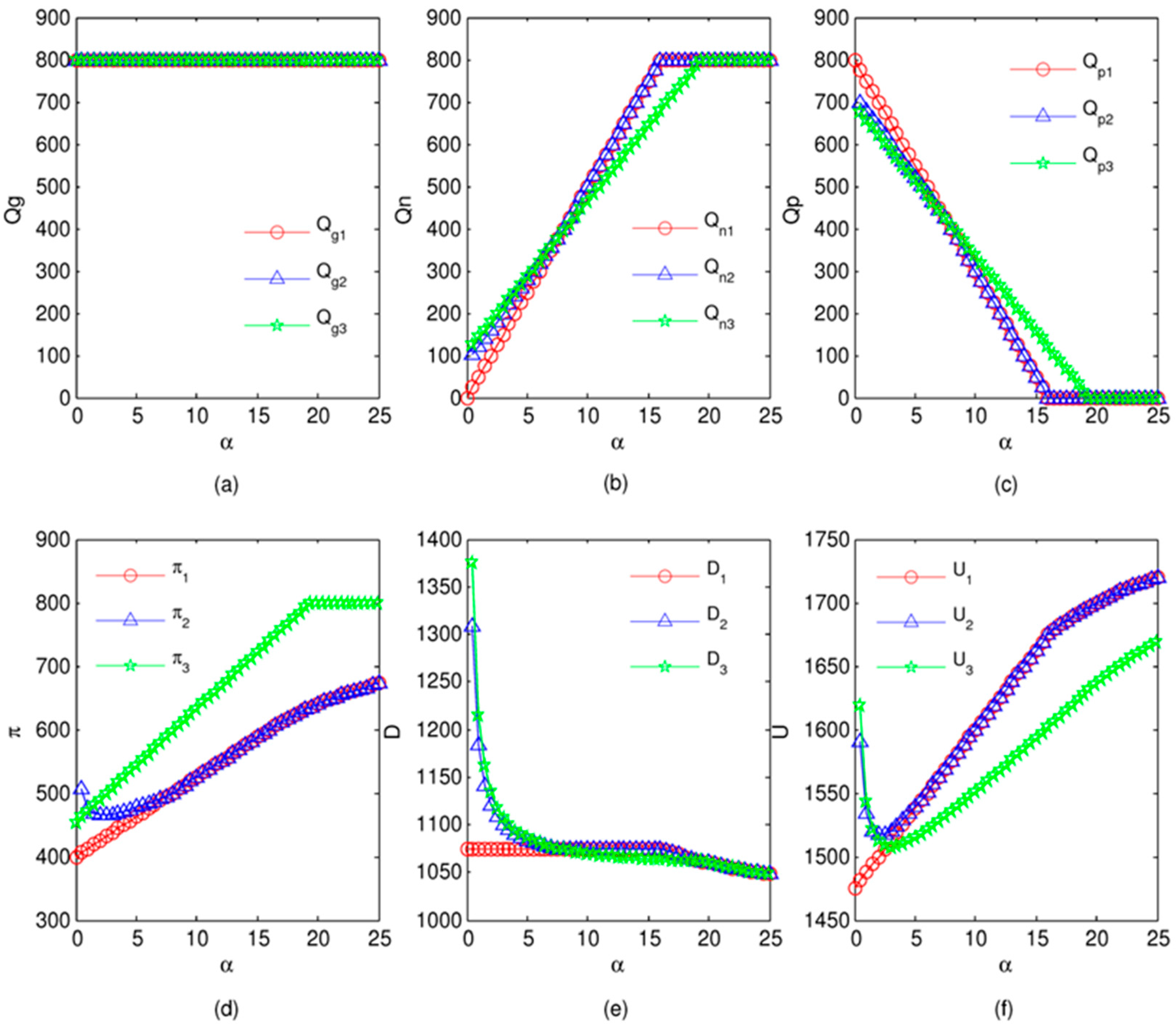
The impact of $\alpha$ on the equilibrium quantity under three scenarios is mainly illustrated in the first three figures above. From Figure 2a, we assume that $q_1,b_1,p$ are constants, so the quantity of users who exhibit the behavior of PT is also a constant. Figure 2b shows that the quantity of users who exhibit the behavior of IPT in scenario three is greater than the other two scenarios when $\alpha <7.5$; while it is less than the other two scenarios when $\alpha >7.5$. Figure 2c shows that the quantity of users who exhibit the behavior of FPT in scenario three is less than the other two scenarios when $\alpha <7.5$; but it is greater than the other two scenarios when $\alpha >7.5$. In addition to that, when $\alpha >19.4$, quantities of users who exhibit the behavior of IPT and FPT in these three scenarios are equal to that of PT and zero respectively. That is, when the PS of leisure travelers is far greater than commuters, the self-resetting of the BSS can be realized in all three scenarios.

The remaining figures above show the impact of $\alpha$ on surplus values and profits, respectively. Figure 2d shows that the operator gets more profit in scenario three compared to the other two scenarios when $\alpha \ge 1$ ($\alpha \approx 1$ is the intersection point of the yield curve between scenario two and three). When $\alpha <1$, the operator’s profit in scenario two is greater than others. Figure 2e shows that surplus value of users in scenario two and three are far greater than the scenario one when $\alpha <7.5$; when $\alpha >7.5$, the surplus value of users in these three scenarios is almost the same. Figure 2f shows that the profit of the government in scenario two and three are greater than one when $\alpha <2.5$, and the profit of the government in scenario one and two are far greater than three when $\alpha >2.5$.

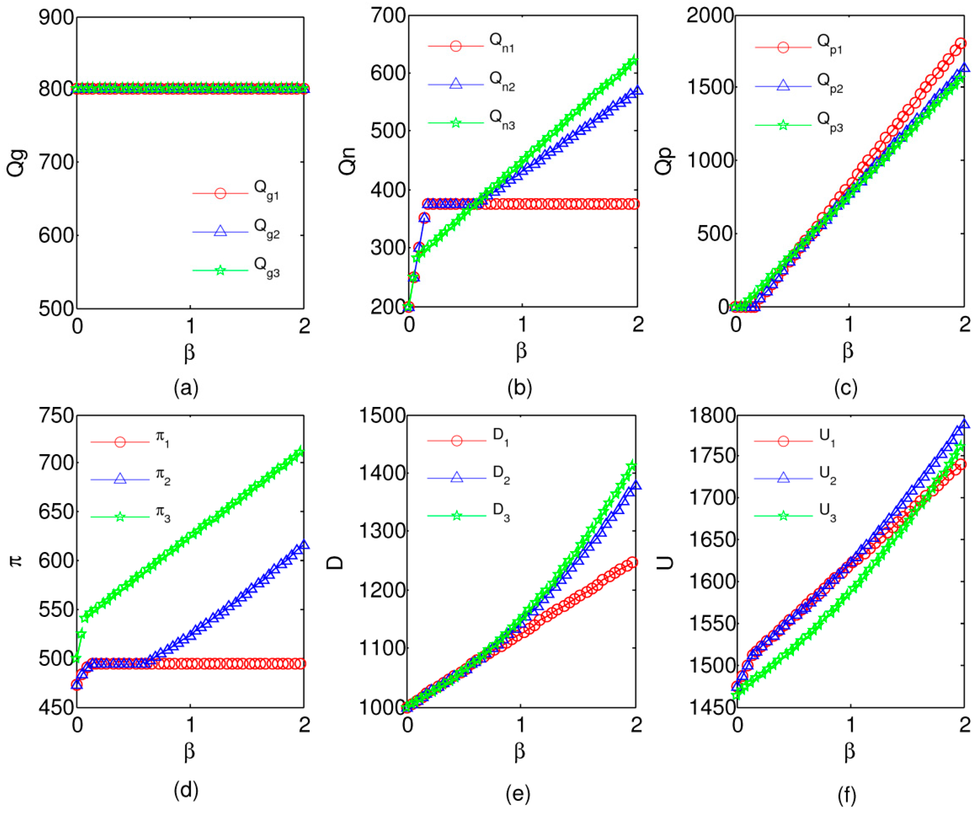
The impact of $\beta$ on the equilibrium quantity under three scenarios is mainly illustrated in the first three figures above. As seen from Figure 3b, the quantity of users who exhibit the behavior of IPT in scenario one and two are greater than three when $\beta \le 0.6$; while scenario two and three are greater than scenario one when $\beta >0.6$. Figure 3d shows that the profit of the operator in scenario three is much greater than the others. In Figure 3e, it shows that the surplus value of users in these three scenarios are all the same when $\beta \le 0.6$, while the scenario two and three are greater than one when $\beta >0.6$. Figure 3f shows that profit of the government in these three scenarios is relatively close.

We summarize our findings based on above numerical examples as follows:

(1)

When BIM is implemented in the BSS, the profit of the operator and the government are improved;

(2)

When $\alpha$ is small, the strategy in scenario two is the best;

(3)

When $\alpha$ is moderate, the strategy in scenario one is the best under the setting $\beta \le 1-\frac{2b_{1}p}{q_1}$; while the strategy in scenario three is the best under the setting $\beta >1-\frac{2b_{1}p}{q_1}$;

(3)

When $\alpha$ is large, there is no difference on the incentive effect of implementing the BIM among these three scenarios. However, scenario three is greater than the others on the operator’s profit side.

5. Case Discussion

In order to find more specific implications and suggestions to make the BSS practicable in the real life, we conduct a questionnaire survey of the users’ travel behavior of BSS in Fuzhou, China. This survey shows the number of leisure users in the BSS is less than commuters ($\beta$ = 0.3). Moreover, we find the age of leisure travelers (45.2 years old) is older than commuters (34 years old). In China, older consumers always have higher price sensitivity than younger consumers [32]. The tough living environments for the old Chinese generation in their childhood mainly lead their saving habits. This causes most of them to be more sensitive in price. However, for most of young people, especially those who born after 1980s, they are less sensitive to the price of goods because of better living condition. Therefore, the PS of leisure travelers is greater than commuters in Fuzhou. According to the numerical analysis, the best decision for the BSS in Fuzhou is to implement the BIM by the operator without subsidy. Furthermore, we find that 64.3% of users choose to use public bicycles during peak hour, only 6% of them choose to avoid peak time. This demonstrates that, without the incentive for leisure travelers, they might travel in rush hour; however, they may change their travel behavior according to the requirement of the BSS with an incentive.

For comparison of $\beta$ in different types of cities, we collect the second-hand data in the BSS of four cities in China. Statistical results are shown in

Table 3. Statistical results of the quantity of leisure travelers and commuters.

City	Commuter	Leisure Traveler	$\mathit{\beta }$	Data Source (Questionnaire Survey)	Implementation Suggestion
Guangzhou	73.0%	27.0%	0.37	Investigation report	Without subsidy
Hangzhou	40.0%	60.0%	1.50	Article	Subsidize the IPT
Nanjing	64.2%	35.8%	0.56	Investigation report	Any one
Fuzhou	76.8%	23.2%	0.30	Questionnaire data	Without subsidy
Zhangjiagang	46.2%	53.8%	1.17	Master thesis	Subsidize the IPT

.

In Table 3, we find that the quantity of commuters is larger than leisure travelers in Guangzhou (large sized city) [33]. According to our numerical analysis, the best strategy is to implement the BIM by operator without subsidy (Scenario one). The quantity of commuters is less than leisure travelers in Zhangjiagang (small sized city) [34]. Thus the best strategy is for the government to directly subsidize users who exhibit travel behavior of IPT (Scenario three). Although Hangzhou is the same size as Nanjing and Fuzhou (medium sized cities), the quantity of commuters in Hangzhou is significantly less than leisure travelers [35], which is opposite to the other two cities [36]. This difference is mainly caused by the purpose of this city: tourism. Here a lot of users use public bicycles for travelling and sightseeing. Therefore, the best strategy for Hangzhou is the same as Zhangjiagang. As for Nanjing, the implementation effects are almost the same in different strategies.

Based on travel data of users, the BSS supervisors can decide how to implement the BIM by finding the corresponding strategy from our numerical analysis.

6. Concluding Remarks

Rebalance of bicycles during rush hour has been one of the major concerns in BSS. In order to solve this concern, we divide users in a BSS into two types: leisure travelers and commuters. The service provider, such as the operator and the government could implement BIM. The aim of this is to stimulate leisure travelers to actively respond to the bicycle resetting needs in a BSS, and guide commuters to avoid travelling during rush hour. By implementing BIM with suitable method, the operator and the government could reduce the bicycles scheduling pressure during rush hour, and even realize the self-resetting of the BSS. In this paper, we propose BIM implementation under three scenarios through cooperation between the government and the operator. Scenario one is the implementation of BIM by an operator without a subsidy. Scenario two is the implementation of BIM by an operator with a subsidy. Scenario three is the implementation of BIM by a direct government subsidy to the users who exhibit travel behavior of IPT. A Stackelberg game model is analyzed between the operator and the government in a two-echelon BSS. We use the backward induction to obtain the best response functions of system members. Furthermore, numerical examples are used to illustrate the impact of two important parameters on quantities of users’ different travel behaviors, the surplus values of these users, and profits of the operator and the government in these three scenarios. Then we use questionnaire survey in Fuzhou, and collect some second hand data from four representative cities in China, to study travel behaviors of users in a BSS.

We find that:

(1)

The government and the operator can implement BIM to relieve rebalance pressure of bicycles in a BSS. Meanwhile, the benefit of all stakeholders has been enhanced.

(2)

In the developed region, the PS of commuters is greater than leisure travelers. The strategy of implementing BIM by the operator with government subsidy is the best way.

(3)

In the developing region, the PS of leisure travelers is always greater than commuters. The strategy of implementing BIM by the operator without subsidy is the best choice to the large and medium-sized city. The fast pace lifestyle in these cities leads to a large number of commuters. Therefore, the incentive effect is not very obvious in this case. However, as for the small sized or tourist city, the strategy in scenario three (the implementation of BIM by the government direct subsidy to users who exhibit travel behavior of IPT) is the best choice. In these cities, the proportion of leisure travelers is always larger than 50%, resulting in significant incentive effect. Thus, the subsidy from government plays an important role under this case.

In the past year, there has been growing attention on exploiting potentialities of dynamic pricing for BSS. Some of the BSS worldwide have made successful achievements. For example, London’s Barclay’s Cycle Hire system has applied a reward incentive method to minimize its operating costs. Pfrommer et al. found that the user-rebalancing incentives-scheme were viable option when the number of commuters was not much greater than leisure travelers [37], which is similar to our research results. Moreover, the “Reverse Riders Rewards” program provides incentive for users to self-balance their system during rush hour. It has been carried out by some cities, such as Paris, Beijing, cities in North American, etc. [38]. Therefore, we suggest it would be helpful to apply BIM in the BSS and other similar systems.

Possible extension could be to consider the incentive mechanism of public transportation. In particular, consider different types of travel behavior and their VOT. The VOT are significantly different according to various trip intentions of users in a BSS. They will affect the benefit of stakeholders in a further way. We consider the PS in this paper. Another interesting extension is to consider both the PS and VOT.