The Design of a Sustainable Location-Routing-Inventory Model Considering Consumer Environmental Behavior

Abstract

Our aim is to design a sustainable supply chain (SSC) network, which takes into consideration consumer environmental behaviors (CEBs). CEBs not only affect consumers’ demand for products with low carbon emissions, they also affect their willingness to pay premium prices for products with low carbon emissions. We incorporate CEBs into the SSC network model involving location, routing and inventory. Firstly, a multi-objective optimization model comprised of both the costs and the carbon emissions of a joint location-routing-inventory model is proposed and solved, using a multi-objective particle swarm optimization (MOPSO) algorithm. Then, a revenue function including CEBs is presented on the basis of a Pareto set of the trade-off between costs and carbon emissions. A computational experiment and sensitivity analysis are conducted, employing data from the China National Petroleum Corporation (CNPC). The results clearly indicate that our research can be applied to actual supply chain operations. In addition, some practical managerial insights for enterprises are offered.

1. Introduction

Along with the heightened concerns over the past few decades relating to sustainable supply chains (SSC), governments, enterprises and consumers are becoming increasingly aware of the need to reduce carbon emissions. Governments have introduced a number of regulations, such as carbon taxes, cap-and-trade mechanisms and carbon constraints to mandate carbon emission reductions in SSC management [1]. In addition, a few socially responsible enterprises have engaged in voluntary emission reduction programs. Companies such as BP and Nike have taken actions to reduce emissions in order to improve their public image. Wal-Mart and Tesco require their suppliers to reveal their carbon emissions on product labels, where they can be seen by consumers and society. In addition, consumers with higher levels of environmental consciousness are willing to pay a premium price for low carbon products [2,3,4,5]. The demand for low carbon products has become greater and greater [6,7,8]. It can be safely assumed that low carbon products will become more competitively priced in the future. Clearly, the drive for environmental improvement is increasing.

Traditionally, a supply chain network design problem focuses on minimizing the fixed and operational costs that companies directly incur. Only recently, however, have some studies started taking carbon emissions into account [9,10,11]. Many studies indicate that there is a trade-off between the environment and economics in a supply chain [12,13,14]. However, it is possible to significantly reduce carbon emissions without greatly increasing costs, using proper supply chain operations [15,16]. In general, there is a paradox between cost and carbon emissions in SSC management.

Companies are never going to reduce their carbon emissions until factors such as cost, profits, brand awareness and consumer pressure are involved. Currently, the main drive for carbon emission reduction can be classified into two categories. The first is mandatory emission reductions, which includes features such as carbon taxes and carbon cap policies [17]. This approach to carbon emissions is punitive. The alternative method is to encourage enterprises to voluntarily reduce their carbon emissions. This encouragement, in turn, can take the form of two types of motivation. One type is through policies such as carbon allowances and cap-and-trade mechanisms. The second type takes on board market considerations. For example, studies have shown that green products have the marketing potential to endow an enterprise with a good public image, which in turn can improve the relevant products’ pricing structure or increase consumer demand [8,18]. Looking further into the future, the effects of exploiting the marketing potential of products with low carbon emissions will increase substantially. Creating a SSC network is both a challenge and an opportunity. Presumably, the information already available to society at large has made consumers more environmentally mature, and these mature consumers would like to purchase products with smaller carbon footprints. In this study, we propose the design of a SSC network from a market-driven perspective. Specifically, the purpose of this study is to optimize the profitability of a company through CEB. We decide on the design of the SSC network after considering the number and location of warehouses, the routes from manufacturers to warehouses and from warehouses to retailers, and the inventory polices of the various facilities. Firstly, a multi-objective model is constructed to create a trade-off between cost and carbon emissions. Then, a general revenue objective factoring in CEBs is modeled, based on the relationship between cost and carbon emissions. This study allows us to achieve the best of both worlds, i.e., maximizing the profits of companies, while reducing carbon emissions as much as possible. These achievements also represent the main points of innovation in this paper.

The remainder of the paper is organized as follows: Section 2 reviews the relevant literature. Problem descriptions and assumptions are presented in Section 3. Section 4 describes the multi-objective model that creates the trade-off between cost and carbon emissions, and then constructs the general revenue objective function taking CEBs into consideration. The approach used as a solution for the model is given in Section 5. Results of the computational experiment and a sensitivity analysis are conducted in Section 6; the managerial insights are also illustrated in this section. Finally, our conclusions are presented in Section 7.

2. Literature Review

A key driver of any supply chain is its distribution network. This network, however, is generally also the main source of carbon emissions. The operations of a supply chain network consist of three major components, namely location, routing and inventory (LRI). However, most existing literature integrates only any two of the above, i.e., location-routing problems [19], inventory-routing problems [20], and location-inventory problems [21], as their target topics. Ahmadi-Javid and Azad [22] presented for the first time a model to simultaneously optimize location, routing and inventory decisions in a supply chain network. Ahmadi-Javid and Seddighi [23] studied a ternary integration problem that incorporated location, routing and inventory decisions in designing a multi-source distribution network. They then solved the model using a three-phase heuristic. On the whole, very few researchers have studied the ternary integration LRI problem, and fewer still have incorporated carbon emissions into an LRI problem when designing a supply chain network. This is a very important issue, which has unfortunately been largely ignored.

Numerous studies concentrate on the trade-off between the environment and the economy in supply chain management [12,24]. According to the most recent papers, three types of research have been conducted and corresponding suggestions made: (i) Translate carbon emissions into cost by introducing carbon regulations, such as a carbon tax, cap-and-trade mechanisms, etc. Kroes et al. [25] investigated the relationship between a firm’s environmental performance compliance and their marketing success in the context of stringent cap-and-trade regulations. Benjaafar et al. [12] presented a cost optimization model via translating carbon emissions into unit costs by carbon price. The two studies proved that there is a close relationship between economic costs and carbon emissions. Similar research was conducted by Hua et al. [24], which studied managing carbon footprints in an inventory system under a carbon emission trading mechanism. (ii) A mandatory carbon cap is used to reduce emissions. This policy specifically prohibits companies from emitting any carbon emissions in excess of their carbon cap. Diabat et al. [26] proposed a mixed-integer program model with carbon cap constraints when designing a supply chain network. A carbon-constraint economic order quantity (EOQ) model was provided to reduce emissions by properly adjusting order quantities [16]. The effects of carbon-constraint measures are significant. However, it is relatively difficult to implement such policies, as they are currently unacceptable to many companies. Businesses, which are profit-driven, lack the motivation to participate in this non-profitable activity. (iii) Provide a set of Pareto solutions, which shows the trade-off between cost and carbon emissions. The advantage of this method is that it can give a set of non-dominated solutions. In addition, the decision makers can choose their preferred configuration. Wygonik and Goodchild [27] presented trade-offs between cost, service quality and the carbon emissions of an urban delivery system. Wang et al. [28] provided a bi-objective optimization model for a green supply chain network design. One of the two objectives was cost minimization; the other was to minimize carbon emissions. The Pareto results showed that the bi-objective model is an effective tool for solving this kind of problem. However, the terminal decision will be made by managers, and thus, personal preferences will inevitably be involved.

The worldwide reduction framework would involve drawing more companies into carbon reduction activities and also into assuming social responsibilities. In order to determine how to make enterprises voluntarily reduce emissions in the context of an earnings-dominated market, it is first necessary to learn how best to improve the potential motivation for corporations to reduce their carbon emissions. The use of carbon labeling is an effective means to encourage consumers to buy environmentally friendly products. There is, however, a definite need to better understand consumers’ responses to eco-labels [28]. Consumers’ willingness to pay a premium price for products with lower carbon emissions has been shown to be increasing [4,29]. Vanclay et al. [30] defined three levels of carbon labeling (from low to high) as green, yellow and black. They then found that after labeling, the black-labeled (highest carbon emission) product sales decreased by six percent, while green-labeled product sales increased by four percent, when all other conditions were basically unchanged. These results imply that the potential effectiveness of carbon labels in emission reductions is significant. However, green products usually cost more than conventional products, which in turn makes green goods more expensive [3].The key issue is whether consumers will be willing to pay a premium price for the green goods. If not, governments may have to subsidize producers who manufacture green products [5]. Some studies have shown that the higher the CEBs, the higher the price consumers are willing to pay for environmentally friendly products [2].

Economic globalization and rapid high-tech development have intensified market competition to unprecedented levels. New patterns of product competition will emerge over the next few years, and the manufacture of green products as part of that competition is an irresistible trend. Conrad [3] studied the effects of consumer environmental concerns on price, choice of product and market share in the context of duopoly. Liu et al. [8] proved that, as consumers’ environmental awareness increases, retailers and manufacturers with superior eco-friendly operations will benefit in the long run. A model considering the effect of environmental conscious consumers on firms’ adoption of cleaner technologies showed that, as pollution intensifies, consumers play a much more positive role in the companies’ environmental activities. The consumers’ attitudes encourage firms to reduce carbon emissions, even in the absence of emission regulations [7]. However, many studies focus on emission reduction through governmental regulations, and rarely through market forces [31]. Actually, consumer response and preference for greener products, as well as market competition, combine to strongly encourage companies to adopt environmentally friendly operations.

By reviewing previous studies, we find that very little research has been conducted on LRI optimization as a means to minimize carbon emissions. Fewer still have incorporated CEBs into a revenue model. Indeed, most studies fail to properly integrate market-driven factors—in particular CEBs—and LRI operations and revenue objectives with cost-environment trade off. In this paper, we make the following contributions: (i) The concept of consumer environmental behaviors (CEBs) was proposed and incorporated into a revenue function. CEBs not only affect consumers’ demand for low carbon emission products, but also their willingness to pay a premium price for low carbon emission products. (ii) A multi-objective mixed-integer formulation for the trade-off between cost and carbon emissions was presented first. The solution was then found using the multi-objective particle swarm optimization (MOPSO). Hence, a set of distributed Pareto optimal solutions can be obtained. On this basis, revenue function can be maximized. (iii) We conduct a computational experiment based on data from the China National Petroleum Corporation (CNPC) to test the presented models. Then, the Pareto solutions are presented. In addition, a number of sensitivity analyses are implemented on multiple variables. Hence, we obtain interesting managerial insights that may be of use to logistics service firms.

3. Description and Assumptions

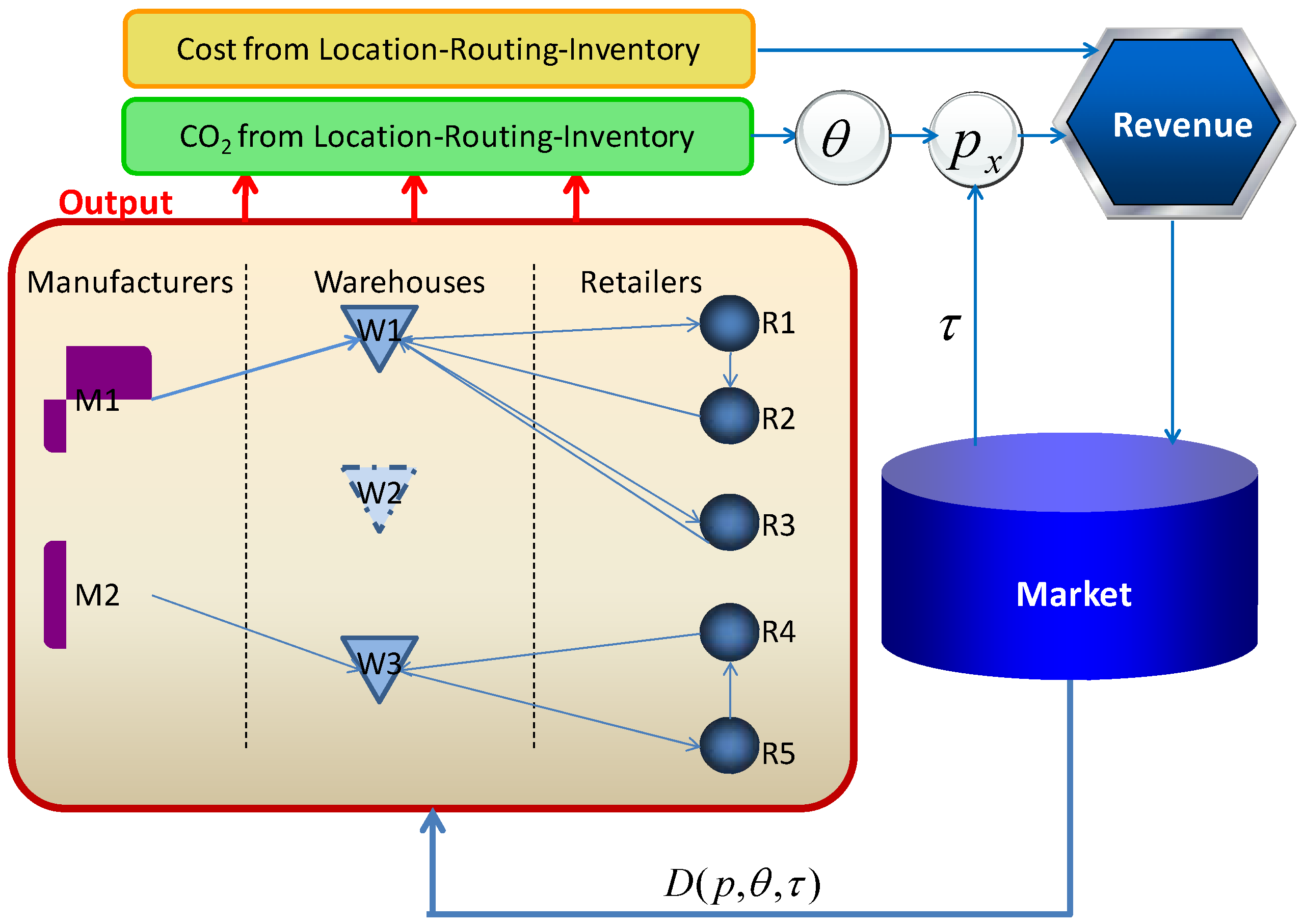
3.1. Problem Description

For a supply chain network consisting of manufacturers (M), warehouses (W) and retailers (R), the location of warehouses is potentially significant. In addition, each warehouse has a specific capacity level, which makes the supply chain network more realistic. The goals of our model are to choose and allocate warehouses, schedule vehicle routes and determine an inventory policy to meet retailers’ demands taking into consideration CEBs. The framework of the problem is depicted in Figure 1.

In Figure 1, the operations generate cost and CO₂ in a supply chain network involving location, routing and inventory. $\mathsf{\theta }$ is the green level coefficient of products, which is decided by the CO₂ emissions from the LRI operations, which can in turn be calculated by Equation (14); $\tau$ is the consumer environmental behaviors (CEBs), and a larger $\tau$ indicates that consumers are willing to pay a higher premium for greener products. CEBs can be calculated as $\tau ={\displaystyle {\int }_{\underset{\_}{g}}^{\overline{g}}\tau (g)\mathsf{\beta }}$, where $\mathsf{\tau }(g)$ is the CEBs of consumer group $g$, $\mathsf{\beta }$ is a correction factor of CEBs over time. We assume $\mathsf{\beta }\ge 1$, because CEBs would not decrease over time; $\underset{\_}{g}$ is the consumer group with the worst CEBs, and $\overline{g}$ is the consumer group with the best CEBs. $p$ is the price of the product, which is decided by $\mathsf{\theta }$ and the CEBs $\tau$. The market demand of a product depends on $\mathrm{p}$, $\mathsf{\theta }$ and $\tau$. Conversely, operation-induced emissions and cost will be influenced by the market, which is important, especially in a situation of oversupply. To maximize profits, supply chain enterprises will certainly endeavor to meet consumers’ preferences, so as to improve their businesses’ performance.

3.2. Assumptions

We assume that the consumers are under symmetric information regarding products’ carbon emissions. With the preferences displayed by CEBs, we aim to find the optimal supply chain network design and operational strategy.

(i)

In this paper, the CEB choices focus on the carbon emissions from the LRI, including sourcing, production and/or recovery. It is reasonable to choose supply chain services as the study object, as they represent a major source of carbon emissions.

(ii)

There is no difference among delivery routes, and the road conditions are nearly the same. In other words, the carbon emissions and costs are only affected by the distance travelled.

(iii)

Each warehouse is assumed to follow a $(Q,R)$ inventory policy. That is, when the inventory of a warehouse reaches the reorder point $R$, a fixed quantity $Q$ is ordered from the upper stream plant.

(iv)

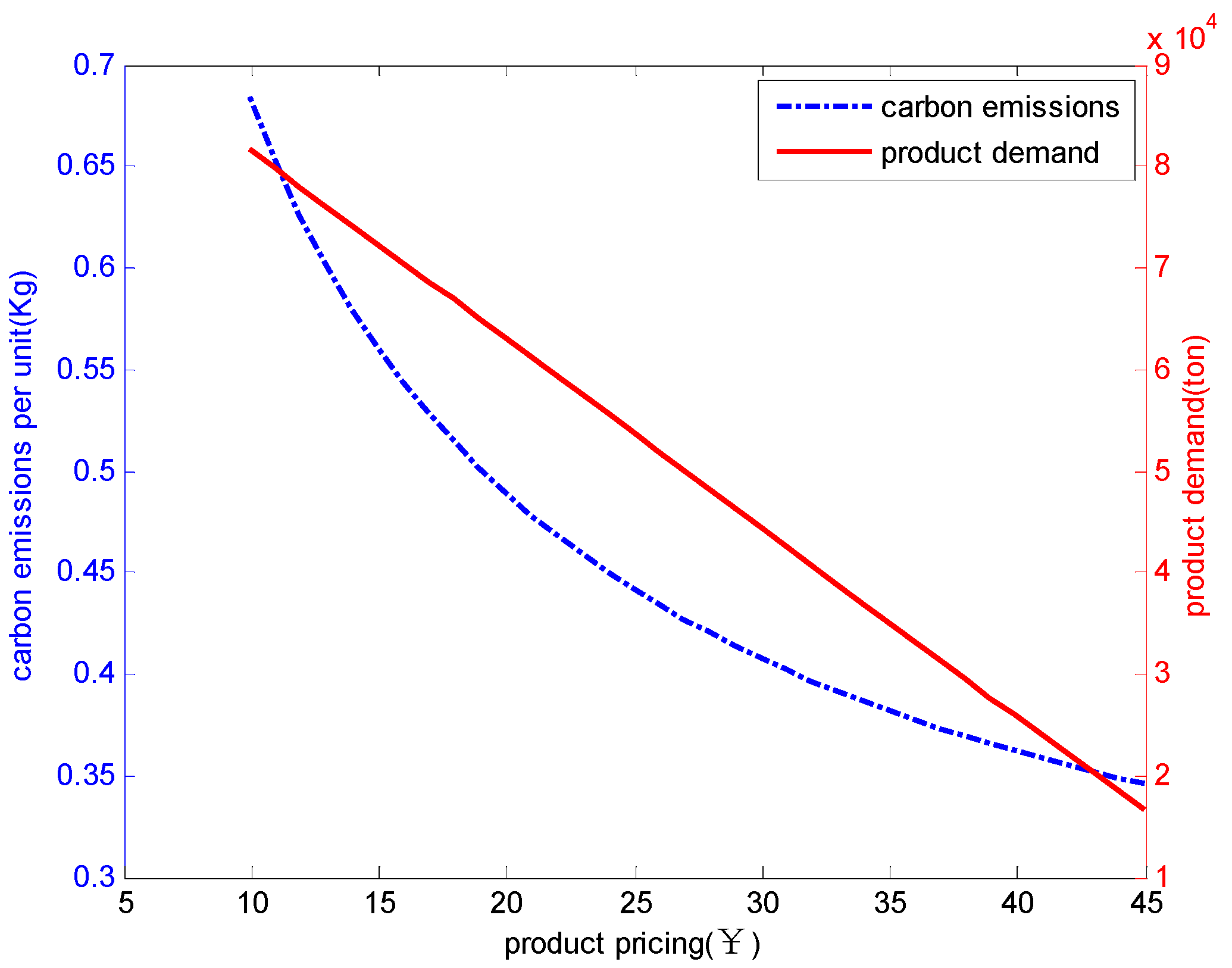
The discussed products/services are in an oversupplied market. CEBs are in positive correlation with market demand. We assume the consumer demand function is expressed as:

$$D(p_x,\mathsf{\theta },\mathsf{\tau })=D_0-{\mathsf{\lambda }}_1{p}_x+\frac{1}{2}{\mathsf{\lambda }}_2\mathsf{\tau }\mathsf{\theta }$$

(1)

where D₀ is the initial demand without considering CEBs or a premium for greener products, λ₁ is the market inverse demand coefficient, λ₂ is the attraction coefficient with the environmentally friendly level of products, and τ is the consumers’ environmental preference for low carbon products. Obviously, the market demand is a decreasing function of price, and an increasing function of $\mathsf{\theta }$ and τ.

4. The Model

4.1. A Multi-Objective Model for Cost and Carbon Emissions

There is a trade-off between cost and carbon emissions in supply chain operations. Generally, a set of optimal Pareto solutions $(c_x,e_x)$ can be obtained, and particularly, the extreme values on the Pareto curve are $(\underset{\_}{c},\overline{e})$ and $(\overline{c},\underset{\_}{e})$. The aim of this paper is to find the optimal solution $({c_x}^{*},{e_x}^{*})$ in the supply chain; one which will maximize profits while taking CEBs into consideration. For these operations, we should make the following decisions:

(i)

Location decisions—how many warehouses should be opened, and where to locate the opened warehouses.

(ii)

Routing decisions—how to assign the vehicle routes from manufacturers to warehouses (M-to-W) and from warehouses to Retailers (W-to-R).

(iii)

Inventory decisions—what is the order quantity, and how many safety stocks should be maintained?

(iv)

What is the most appropriate level of green to choose?

Thus, the decision variables can be denoted as

$$y_j=\{\begin{array}{ll}1,\hfill & \text{if warehouse} j\hspace{0.17em}\text{is}\hspace{0.17em}\text{opened}\hspace{0.17em}\hfill \\ 0,\hfill & \text{otherwise}\hfill \end{array},j\in J$$

$$x_{ji}^r=\{\begin{array}{ll}1,\hfill & \text{if} \text{retailer} i\hspace{0.17em}\text{is}\hspace{0.17em}\text{assigned}\hspace{0.17em}\text{to}\hspace{0.17em}\text{warehouse} j\hfill \\ 0,\hfill & \text{otherwise}\hfill \end{array},i\in I,j\in J$$

$$x_{kj}^p=\{\begin{array}{ll}1,\hfill & \text{if}\hspace{0.17em}\text{warehouse} j\hspace{0.17em}\text{is}\hspace{0.17em}\text{assigned}\hspace{0.17em}\text{to}\hspace{0.17em}\text{manufacture} k\hfill \\ 0,\hfill & \text{otherwise}\hfill \end{array},j\in J,k\in K$$

$$z_{miv}=\{\begin{array}{ll}1,\hfill & \text{if}\hspace{0.17em}m\hspace{0.17em}\text{precedes}\hspace{0.17em}i\hspace{0.17em}\text{in}\hspace{0.17em}\text{the route}\hspace{0.17em}\text{of}\hspace{0.17em}\text{vehicle}\hspace{0.17em}v\hfill \\ 0,\hfill & \text{otherwise}\hfill \end{array},\forall m\in (I\cup J),i\in I.$$

$Q_j$ is the order quantity of warehouse $j$.

The multi-objective function includes cost and carbon emissions from location, routing and inventory. First, the cost is composed using the following terms:

(i)

Location cost. The cost of warehouse location is ${\displaystyle \sum _{j\in J}{f}_j{y}_j}$, where $f_j$ is the single cost of opening warehouse $j$.

(ii)

Routing cost occurs in the distribution from M-to-W and from warehouse to retailer (W-to-R), which are ${\displaystyle \sum _{k\in K}{\displaystyle \sum _{j\in J}{t}_1{d}_{kj}{x}_{kj}^p}}$ and ${\displaystyle \sum _{j\in J}{\displaystyle \sum _{i\in I}{\displaystyle \sum _{m\in (I\cup J)}{t}_2{d}_{mi}}{z}_{miv}}}$, respectively, where $t_1$ is the M-to-W routing cost per distance; $d_{kj}$ is the distance from manufacturer $k$ to warehouse $j$; $t_2$ is W-to-R routing cost per distance; and $d_{mi}$ is the distance from warehouse $j$ (or retailer $k$ $k$) to retailer $k^{\text{'}}$

(iii)

Inventory cost. Working inventory is ${\displaystyle \sum _{j\in J}{\displaystyle \sum _{i\in I}(h_o\frac{{\displaystyle {\sum }_{i\in I}{\mathsf{\mu }}_i{x}_{ij}^r}}{Q_j}+h_j\frac{Q_j}{2})}}$, and safety stock is ${\displaystyle \sum _{j\in J}{h}_j{z}_{\mathsf{\alpha }}\sqrt{L_j{\displaystyle \sum _{i\in I}{\mathsf{\sigma }}_i^2{x}_{ji}^r}}}$ [22], where $h_o$ is the ordering cost, ${\mathsf{\mu }}_i$ is the demand by retailer $i$, $h_j$ is the hold cost per unit; $L_j$ is the lead time of DC $j$; $z_{\mathsf{\alpha }}$ is left $\mathsf{\alpha }$-percentile of standard normal random variable $Z$, i.e., $P(Z\le z_{\alpha })=\mathsf{\alpha }$ ($\mathsf{\alpha }$ is the desired percentage of retailers’ orders that should be satisfied); ${\mathsf{\sigma }}_i^2$ is the variance of demand from retailer $i$.

The carbon emissions are composed of the following terms:

(i)

Carbon emissions from facilities. The carbon emissions of a warehouse location can be denoted as ${\displaystyle \sum _{j\in J}{\widehat{f}}_j{y}_j}$, where ${\widehat{f}}_j$ is the carbon emissions of building warehouse $j$.

(ii)

Carbon emissions from routing. The routing emissions from the M-to-W and W-to-R transportations are denoted as ${\displaystyle \sum _{k\in K}{\displaystyle \sum _{j\in J}{\widehat{t}}_1{d}_{kj}{x}_{kj}^p}}$ and ${\displaystyle \sum _{j\in J}{\displaystyle \sum _{i\in I}{\displaystyle \sum _{m\in (I\cup J)}{\widehat{t}}_2{d}_{mi}}{z}_{miv}}}$, respectively, where ${\widehat{t}}_1$ is the M-to-W carbon emissions per distance, and ${\widehat{t}}_2$ is the carbon emissions per distance from warehouse $j$ (or retailer $k$) to retailer $k^{\text{'}}$.

(iii)

Carbon emissions from inventory. The inventory emissions come from the working inventory and safety stock, which are ${\displaystyle \sum _{j\in J}{\displaystyle \sum _{i\in I}{\widehat{h}}_j\frac{Q_j}{2}}}$ and ${\displaystyle \sum _{j\in J}{\widehat{h}}_j{z}_{\mathsf{\alpha }}\sqrt{L_j{\displaystyle \sum _{i\in I}{\mathsf{\sigma }}_i^2{x}_{ji}^r}}}$, respectively, where ${\widehat{h}}_j$ is the carbon emissions per holding inventory. It is worth mentioning that carbon emissions from inventory mainly refer to the energy consumption and product emissions during storage.

(iv)

Other emissions, including emissions from purchasing, production and recovery. The purchasing emission is $Pur\text{'}.{\displaystyle \sum _{i\in I}{\mathsf{\mu }}_i}$, where $Pur\text{'}$ is carbon emissions from purchase per unit. The production emission is $Pn\text{'}.{\displaystyle \sum _{i\in I}{\mathsf{\mu }}_{\mathrm{i}}}$, where $Pn\text{'}$ is carbon emissions from production per unit. The recovery emission is $\mathrm{R}cy\text{'}.{\displaystyle \sum _{i\in I}{\mathsf{\mu }}_i}$, where $\mathrm{R}cy\text{'}$ is carbon emissions from recovery per unit.

The multi-objective problem is formulated as follows:

$$\begin{array}{l}\min c_x=({\displaystyle \sum _{j\in J}{f}_j{y}_j}+{\displaystyle \sum _{k\in K}{\displaystyle \sum _{j\in J}{t}_1{d}_{kj}{x}_{kj}^p}}+{\displaystyle \sum _{j\in J}{\displaystyle \sum _{i\in I}{\displaystyle \sum _{m\in (I\cup J)}{t}_2{d}_{mi}}{z}_{miv}}}\hspace{0.17em}+{\displaystyle \sum _{j\in J}{\displaystyle \sum _{i\in I}(h_o\frac{{\displaystyle {\sum }_{i\in I}{\mathsf{\mu }}_i{x}_{ji}^r}}{Q_j}}}\\ +h_j\frac{Q_j}{2})+{\displaystyle \sum _{j\in J}{h}_j{z}_{\mathsf{\alpha }}\sqrt{L_j{\displaystyle \sum _{i\in I}{\mathsf{\sigma }}_i^2{x}_{ji}^r}}})/{\displaystyle \sum _{i\in I}{\mathsf{\mu }}_i}\end{array}$$

(2)

$$\begin{array}{l}\min e_x=({\displaystyle \sum _{j\in J}{\widehat{f}}_j{y}_j}+{\displaystyle \sum _{k\in K}{\displaystyle \sum _{j\in J}{\widehat{t}}_1{d}_{kj}{x}_{kj}^p}}+{\displaystyle \sum _{j\in J}{\displaystyle \sum _{i\in I}{\displaystyle \sum _{m\in (I\cup J)}{\widehat{t}}_2{d}_{mi}}{z}_{miv}}}+{\displaystyle \sum _{j\in J}{\displaystyle \sum _{i\in I}{\widehat{h}}_j\frac{Q_j}{2}}}\\ +{\displaystyle \sum _{j\in J}{\widehat{h}}_j{z}_{\mathsf{\alpha }}\sqrt{L_j{\displaystyle \sum _{i\in I}{\mathsf{\sigma }}_i^2{x}_{ji}^r}})/{\displaystyle \sum _{i\in I}{\mathsf{\mu }}_i}}\end{array}$$

(3)

$$\text{s.t.} Q_j+z_{\mathsf{\alpha }}\sqrt{L_j{\displaystyle \sum _{i\in I}{\mathsf{\sigma }}_i^2{x}_{ji}^r}}\le N_j, \forall j\in J$$

(4)

$${\displaystyle \sum _{i\in I}{\displaystyle \sum _{m\in (I\cup J)}{\mathsf{\mu }}_i{z}_{miv}}}\le V^c, \forall m\in (I\cup J)$$

(5)

$${\displaystyle \sum _{v\in V}{\displaystyle \sum _{m\in (I\cup J)}{z}_{miv}}}=1, \forall i\in I$$

(6)

$${\displaystyle \sum _{j\in J}{\displaystyle \sum _{i\in I}{z}_{jiv}}}\le 1, \forall v\in V$$

(7)

$${\displaystyle \sum _{m\in (I\cup J)}{z}_{miv}-{\displaystyle \sum _{m\in (I\cup J)}{z}_{imv}}}=0, \forall i\in I, \forall v\in V, \forall m\in (I\cup J)$$

(8)

$$R_{iv}-R_{mv}+(n_r\times z_{miv})\le n_r-1, \forall i\in I, \forall m\in (I\cup J), \forall v\in V$$

(9)

$$y_j=\{0,1\}, \forall j\in J, \forall n\in N_j$$

(10)

$$x_{kj}^p=\{0,1\}, \forall k\in K, \forall j\in J$$

(11)

$$x_{ji}^r=\{0,1\}, \forall j\in J, \forall i\in I$$

(12)

$$z_{miv}=\{0,1\}, \forall m\in (I\cup J), i\in I, \forall v\in V.$$

(13)

Equation (2) minimizes the cost of the CLRIP, where the first three terms are the fixed location cost, inventory cost, and routing cost, respectively. Equation (3) minimizes the carbon emissions. Equation (4) restricts the inventory in warehouse $j$ to remain within its capacity $N_j$. Equation (5) restricts the load of each vehicle to within its capacity $V^c$. Equation (6) ensures one and only one vehicle serves any retailer. Equation (7) requires that each vehicle serves no more than one warehouse. The flow conservation Equation (8) states that a vehicle entering a node must also leave the node, so as to ensure the route is circular. The sub-tour elimination Equation (9) guarantees that each tour contains a warehouse, from which the tour originates and some retailers [32], where $R_{iv}$ is an auxiliary variable defined for retailer $i$ for sub-tour elimination in the route of vehicle $v$, $n_r$ is the number of retailers. Equations (10)–(13) enforce the decision variables to remain within their respective domains.

4.2. The Revenue Model Considering CEBs

This study focuses on the effects of CEBs on the task of designing a supply chain network, which includes making LRI decisions. CEBs not only affect consumers’ willingness to pay premium prices for greener products, but they also affect the market demand for such products. This willingness to pay varies greatly across industries and consumer groups and also changes in intensity over time [4]. If anything, carbon emissions due to logistics operations have been a concern for a considerable length of time, as these operations are a major source of emissions. We are interested in determining how to maximize earnings, as well as how to improve competition, through the influence of CEBs in three supply chain network structures which include location, routing and inventory considerations.

As non-green products have already been in circulation for many years, the general optimal decision is based on cost minimization. In this study, however, in addition to cost, we also consider carbon emissions as a benchmark. There is a terminal consumer group with an average CEB in the market. The green level $\mathsf{\theta }$ is closely related to the carbon emissions from the supply chain. It has been proven that the carbon emissions and cost are in negative correlation, and thus, we assume that the optimal cost corresponds to a poor performance in relation to carbon emissions, and vice versa. Specifically, with an operation map, we can connect inputs $[\underset{\_}{c},\overline{c}]$ to corresponding outputs $[\overline{e},\underset{\_}{e}]$. Then $\mathsf{\theta }$ can be denoted as

$$\mathsf{\theta }=\overline{e}/e_x$$

(14)

where $e_x$ is the actual carbon emission, and thus ($\mathsf{\theta }-1$) is the carbon abatement ratio. $p$ is the price of non-green products, $(\underset{\_}{c},\overline{e})$ represents the cost and carbon emissions, and $p_x$ is the price with $(c_x,e_x)$. As we know, the marginal cost of carbon reduction increases by degrees. The “low hanging fruit” effect also indicates that initial basic improvement is easier, but the cleanup is harder. Thus, the above situation is considered, and the price of a product with green level $\mathsf{\theta }$ is

$$p_x=p{\mathsf{\theta }}^2$$

(15)

It is worth noting that product price is a quadratic function of $\mathsf{\theta }$, since the environmental improvement has an increasing marginal cost, and production price is worked out to the costing. The quadratic function is commonly used to describe the cost related to the product’s environmental improvement. That is, each additional increment of emissions reduction is more difficult, and hence costlier to achieve [8]. Also, from the market’s perspective, consumers with CEBs are willing to pay a premium price for green products. The greener the product, the more expensive it will be. In addition, for an advanced green product, too, even a small improvement will result in a significant price increase. This increase is deemed to be reasonable.

The aim is to find an optimal portfolio $(c_x,e_x)$ under this context. The basic profit function can be defined as

$$\prod =(p_x-c_x-c_0)D-\mathsf{\epsilon }$$

(16)

where constant $c_0$ is the unit cost of raw materials, and $\epsilon$ is other expenditure, which can be ignored in most cases.

Substituting Equations (1)–(15) into Equation (16), then:

$$\prod =(p{\mathsf{\theta }}^2-c_x-c_0)(D_0-{\mathsf{\lambda }}_{1}p{\mathsf{\theta }}^2+\frac{1}{2}{\mathsf{\lambda }}_2\mathsf{\tau }\mathsf{\theta })$$

(17)

Based on Equation (17), if there is no CEB, the enterprise loses the motivation to reduce carbon emissions, which is consistent with the traditional model. We assume the traditional model has revenue of ${\Pi }^C$, with the only measure being the cost, and we mark it as model PC. In this condition, $\mathsf{\theta }=1$, $\mathsf{\tau }=0$, thus:

$${\Pi }^C=(p-\underset{\_}{c}-c_0)(D_0-{\mathsf{\lambda }}_{1}p)$$

(18)

Enterprises have an incentive to join in carbon reduction practices only when $\Pi -{\Pi }^c>0$. $c_0$ is the same constant in $\Pi$ and ${\Pi }^c$, and thus can be ignored. Then, enterprises will participate in carbon emissions when $(p{\mathsf{\theta }}^2-c_x)(D_0-{\mathsf{\lambda }}_{1}p{\mathsf{\theta }}^2+\frac{1}{2}{\mathsf{\lambda }}_2\mathsf{\tau }\mathsf{\theta })$ $>(p-\underset{\_}{c})(D_0-{\mathsf{\lambda }}_{1}p)$, and thus $c_x<p{\mathsf{\theta }}^2-\frac{(p-\underset{\_}{c})(D_0-{\mathsf{\lambda }}_{1}p)}{D_0-{\lambda }_{1}p{\mathsf{\theta }}^2+\frac{1}{2}{\mathsf{\lambda }}_2\mathsf{\tau }\mathsf{\theta }}$. Actually, $\mathsf{\theta }$ is a function of $e_x$; the relationship between $c_x$ and $e_x$ is important, and it will be solved in the next section.

5. Solving Approach

5.1. Particle Swarm Optimization Algorithm

The particle swarm optimization (PSO) algorithm was first proposed by Kennedy and Eberhart [32]. It is a population-based optimization technique and is becoming very popular, due mainly to its simplicity of implementation and ability to quickly converge to a reasonably good solution [33]. It has been extensively applied to many complex network optimization problems. In the PSO heuristic procedure, a swarm of particles is retained in the search process. Each particle follows a specific trajectory in the search space, and each step of the particle determines a trial solution. Each particle has knowledge of its previous best experience, as well as the best global experience of the entire swarm. The current best fitness of, i.e., the best solution found so far by particle $p$ is represented by $x_{pbes{t}_p}$, while the global best fitness among all particles is represented by $x_{gbest}$. The velocity and position of particle $p$ at iteration (time) $t$ in dimension $d$ are represented by $v_{pd}(t)$ and $x_{pd}(t)$, respectively. Each particle updates its direction at time $t$ according to Equation (19) in the following [32]:

$$v_{pd}(t)=\mathsf{\omega }{v}_{pd}(t-1)+c_1{r}_1(t)(x_{pbes{t}_{pd}}-x_{pd}(t))+c_2{r}_2(t)(x_{gbest}-x_{pd}(t))$$

(19)

where $\mathsf{\omega }$ is the inertia influencing the local and global ability of the particle; usually a value between 0.2 to 0.6 is recommended; $c_1$ and $c_2$ are cognitive and social learning rates, respectively, and $r_1(t)$ and $r_2(t)$ are two uniform random numbers such that $r_1,r_2\in [0,1]$.

The position of particle $p$ is then updated according to Equation (20) in the following

$$x_{pd}(t)=x_{pd}(t-1)+v_{pd}(t)$$

(20)

The update of velocity and the position process is repeated for every dimension and for all particles in the swarm. Eventually the swarm as a whole, like a flock of birds collectively foraging for food, is likely to move close to an optimum of the fitness function [33].

5.2. The Hybrid PSO

The multi-objective model contains location and routing assignments involving binary decisions. Multi-objective programming problems with binary variables cannot be directly processed using the Multi-objective Particle Swarm Optimization (MOPSO) heuristic procedure. Following Shankar et al. [33], the velocity of a particle should be modified if $x_d$ is binary. The modified velocity can be updated as:

$$v_{pd}(t)=v_{pd}(t-1)+r_1(t)(x_{pbes{t}_{pd}}-x_{pd}(t-1))+r_2(t)(x_{gbest}-x_{pd}(t-1))$$

(21)

where $r_1(t)$ and $r_2(t)$ are two random numbers. The position of particle $p$ can be updated as:

$$x_{pd}(t)=\{\begin{array}{cc}0,& \text{If}\hspace{0.17em}{\rho }_{pd}<s(v_{pd}(t))\\ 1,& \text{If}\hspace{0.17em}{\rho }_{pd}\ge s(v_{pd}(t))\end{array}$$

(22)

where ${\mathsf{\rho }}_{pd}$ is a uniformly distributed random number such that ${\mathsf{\rho }}_{pd}\in [0,1]$ and $s(v_{pd}(t))$ is the probability threshold given by $s(v_{pd})=\frac{1}{1+\exp (-v_{pd}(t))}$. In the MOPSO heuristic procedure, the velocity and positions of the continuous particles are updated according to Equations (19) and (20), respectively, while those of the binary variables are updated according to Equations (21) and (22), respectively.

5.3. An Improved Constraint of the MOPSO

In order to improve the ability of the heuristic procedure to search the edges crossing unconnected parts of the feasible region, and also to obtain global non-dominated solutions, some infeasible solutions that are near the feasible solutions are retained in the swarm at the beginning of the search process. A constraint that restricts the infeasibility degree of the constraints is used. At the end of the solution process, all particles retained in the swarm must be feasible. Any infeasible particles will be deleted from the external file gradually, throughout the progress of the search process. A dynamic self-adapting process is needed to control the infeasibility degree in the heuristic procedure. In the multi-objective programming model, the $\ell \text{th}$ inequality constraint can be written as $g_{\ell }(x)\le 0$ and the ${\ell }^{\prime }\text{th}$ equality constraint can be written as $h_{{\ell }^{\text{'}}}(x)-\mathsf{\delta }=0$. The infeasibility of a trail solution $x$ can be quantized as follows:

$$C(x)={\displaystyle \sum _{\ell }\max (g_{\ell }(x),0)+{\displaystyle \sum _{{\ell }^{\text{'}}}\max (\left|h_{{\ell }^{\text{'}}}(x)-\delta \right|,0)}}$$

(23)

In Equation (23), $\mathsf{\delta }$ is a permissible deviation, such that $\mathsf{\delta }>0$ and is very small. If $x\in X$, $C(x)=0$. A dynamic infeasibility threshold $\epsilon$ is used that guarantees the final solutions are all feasible. This threshold is defined as:

$$\mathsf{\epsilon }=\{\begin{array}{ll}{\mathsf{\epsilon }}_0\times (1-5t/4T),\hspace{0.17em}\hfill & \text{if}\hspace{0.17em}t\le 0.8T\hfill \\ 0,\hfill & \text{if}\hspace{0.17em}t>0.8T\hfill \end{array}$$

(24)

where ${\mathsf{\epsilon }}_0$ is the initial allowable deviation of all the constraints. Obviously, $\mathsf{\epsilon }$ decreases with the increase in the number of evolutionary generations. In the searching process, the solution $x$ is retained if $C(x)\le \mathsf{\epsilon }$; otherwise it is discarded.

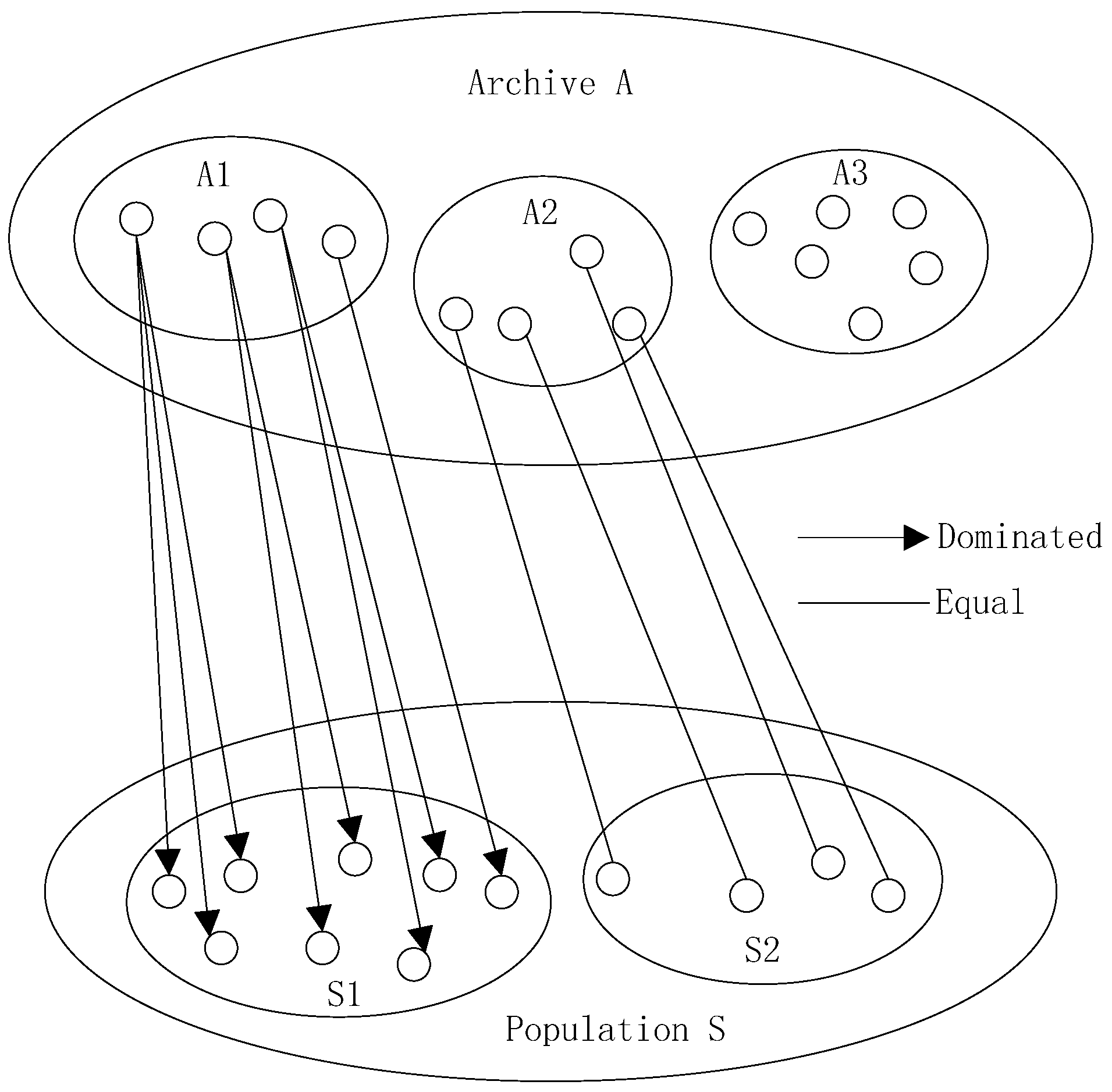
5.4. Selecting the Optimal Particles

The solution of the MOPSO optimization problem is different from a single objective optimization problem. With a single objective problem, it is easy to know which particles are the personal best (pbest) and global best (gbest). With the MOPSO, however, it is difficult to judge which particles are pbest and gbest, because the particles are often non-dominate solutions. However, it is important to pick suitable pbest and gbest particles, since each particle must change its position, as guided by pbest and gbest. Each particle moves toward the non-dominated frontier during the search process [34].

The selection for pbest is relatively simple compared to gbest. A method called Prandom is used in this study, according to which a single pbest is maintained. Pbest is replaced if a new value < pbest, or else, if the new value is found to be mutually non-dominating with pbest, one of the two is randomly selected to be the new best [35]. Before the selection for gbest, there are still some works to illustrate. In the MOPSO algorithm, we usually store the non-dominate solutions in archive, and the archive has a limited capacity. Thus, in order to maintain the archive, the crowding distance should be measured as a base for reserving or discarding non-dominate solutions. The crowding distance $d{t}_{ij}$ can be calculated as:

$$d{t}_{ij}=\sqrt{{\displaystyle \sum _{l=1}^k{f}_l(X_i)-f_l{(X_j)}^2}}$$

(25)

where $f_l(X)$ denotes the objective functions in the dimension $l$. According to Equation (25), the crowding distance matrix can be indicated as:

$$DT=\left[\begin{array}{cccc}d{t}_{11}& d{t}_{12}& \cdots & d{t}_{1n}\\ d{t}_{21}& d{t}_{22}& \cdots & d{t}_{2n}\\ ⋮& ⋮& ⋮& ⋮\\ d{t}_{n1}& d{t}_{n2}& \cdots & d{t}_{nn}\end{array}\right]$$

(26)

where $n$ is the number of non-dominate solutions in the archive. Set S and A represents the populations with particles and archive storing, non-dominate solutions. The particles in S can be divided into two types. One set (S1) is comprised of particles that are dominated by at least one of the non-dominate solutions in A. The other set (S2) is comprised of particles that are not dominated by any one solution in A. $S=S1\cup S2$. In the same way, archive A can also be divided into three types. Set A1 is the non-dominate solutions, which dominate at least one of the particles in S. Set A2 is the non-dominate solutions which have the same position with the particles in S. Set A3 is comprised of the other non-dominate solutions. $A=A1\cup A2\cup A3$. Figure 2 shows the mapping relations of S and A.

For the MOPSO algorithm, the diversity and convergence of population are contradictory issues. One contradiction is the diversity, which guarantees the global best while avoiding the local optimal. The other is the convergence, which promotes particles approaching the Pareto frontier as far as possible. Hence, for particles in S1, if we select non-dominate solutions in A1, which dominate the particles as gbest, the search engines would speed up. However, this can lead to a premature problem. For particles in S2, the global best selection strategy would lead those particles moving to less crowded regions to improve the capability of a global search.

Regardless, each non-dominate solution in the archive has its unique feature. To maintain the diversity of an algorithm, each should have a chance to become a global guide. When paired with these factors, two properties, $f_{ri}$ and $f_{pi}$, are given for non-dominate solutions in the archive. $f_{ri}$ denotes how often the non-dominate solution is selected as gbest, and $f_{pi}$ denotes how many particles in the current population select the non-dominate solution as gbest. Generally, the size of $f_{pi}$ should be restricted. If one gbest is selected by too many particles, the result would be particles converging to a limited region. Based on our experience, we use $f_{pi}\le 0.05N$, where $N$ is the number of particles [36].

Putting the above pieces together, the global best can be selected as follows:

(i)

For each particle in S1, we select a non-dominate solution that randomly dominates the particle from A1 as gbest, but $f_{pi}\le 0.05N$ is necessary. If no solution is found, the gbest should be selected from the A1 with greater crowding distance and smaller $f_{ri}$.

(ii)

For each particle in S2, a random probability model is employed to select gbest from the A2 with greater crowding distance and smaller $f_{ri}$.

The pseudo-code of MOPSO algorithm depicting the entire process is given as follows:

(1)

Initialize positions and velocities of all particles.

(2)

Set the current particle position as Pbest.

(3)

While (iter_count < T)

(4)

for each particle (i = 1:n)

(5)

Select a gbest from the archive.

(6)

Update velocity and position.

(7)

Evaluate the fitness values of the current particle i.

(8)

Update the pbest of each particle by comparison criteria.

(9)

End for

(10)

Update archive by non-dominate solutions.

(11)

For each particle in archive

(12)

If $f_{pi}\le 0.05N$

(13)

Select a dominate solution with greater crowding distance and smaller $f_{ri}$ from archive as gbest randomly.

(14)

End if

(15)

End for

(16)

Output

(17)

End while

6. Computational Experiment

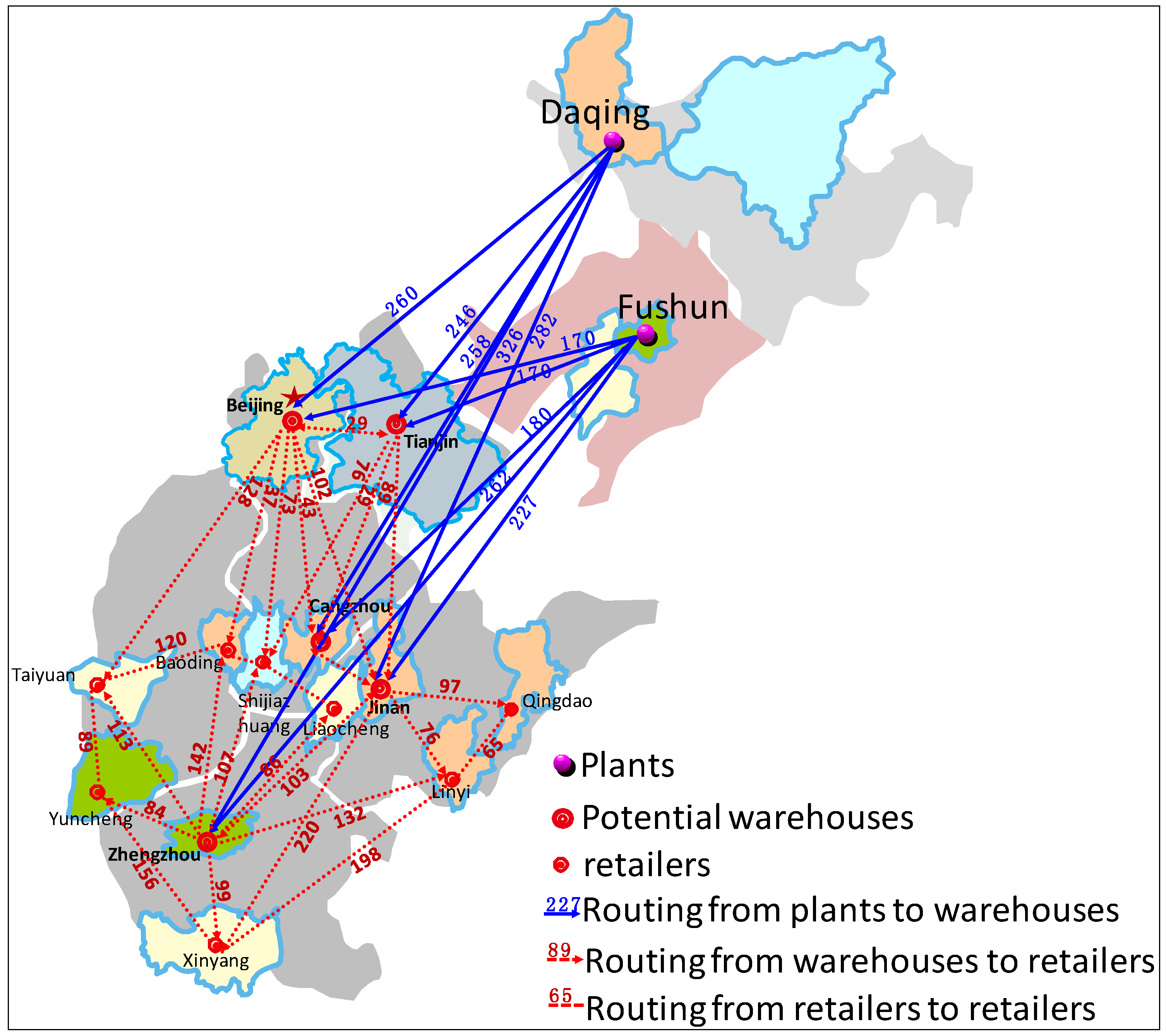
In this section, we evaluate the presented model using a set of numerical data from a real case. The problem is solved by the MOPSO method with Matlab 7.01 on a PC with Intel core i5 and 2.4 GHz. Then, the effects of CEBs and green levels on the decision process are comprehensively analyzed. Finally, some managerial insights are presented.

6.1. Case Study

We consider the experiment based on a case study from the petrochemical industry. Specifically, data from the Northeast Chemical Sales Company of the China National Petroleum Corporation (CNPC) (Beijing, China) was studied. CNPC is a large group, and its supply chain network is responsible for transporting petrochemicals from plants, via warehouses, to retailers. This transportation operation involves location, routing and inventory decisions, as well as the creation of considerable carbon emissions. In this paper, a section of the operational data was analyzed. Specifically, this case study involves two plants, five potential warehouses with retailing functions and eight retailers. Each trajectory is relative to a routing cost and the amount of carbon emission. The routings and distances are shown in Figure 3. The parameters of the warehouses and retailers are listed in

Table 1. The parameters of potential warehouses.

	Beijing	Tianjin	Cangzhou	Jinan	Zhengzhou
Lead time(days)	3	5	6	4	8
Demand variance	12	14	9	11	8
Service level	95%	95%	95%	95%	95%

,

Table 2. The area and fixed location cost of potential DC.

	Area of Location (m2)	Fixed Location Cost (¥)	Hold Cost (¥/ton Day)
Beijing	3000	2,000,000	0.3
Tianjin	3600	1,800,000	0.25
Cangzhou	4000	1,120,000	0.3
Jinnan	4200	1,560,000	0.25
Zhengzhou	5000	1,870,000	0.3

and

Table 3. The parameters of retailers.

	Beijing	Tianjin	Baoding	Cangzhou	Shijiazhuang	Jinan	Liaocheng	Linyi	Qingdao	Xinyang	Zhengzhou	Taiyuan	Yuncheng
Initial demand	430	416	463	577	506	509	522	439	536	696	589	554	694
Service level	92%	91%	95%	95%	90%	98%	91%	94%	95%	95%	95%	95%	90%
Demand variance	9	12	7	8	14	6	6	9	9	11	9	7	9

. In addition, the market inverse demand coefficient is set as 5500, and the attraction coefficient with the environment level of products is set as 5000. CEB is 1, and the routing cost per distance of M-to-W and W-to-R are all equal to q. The order cost is 500, and the capacity of each vehicle is 1500. In addition, ${\widehat{f}}_j^A=29.3N_j$, the carbon emissions per distance are 0.17, and the carbon emissions per inventory are 0.00276.

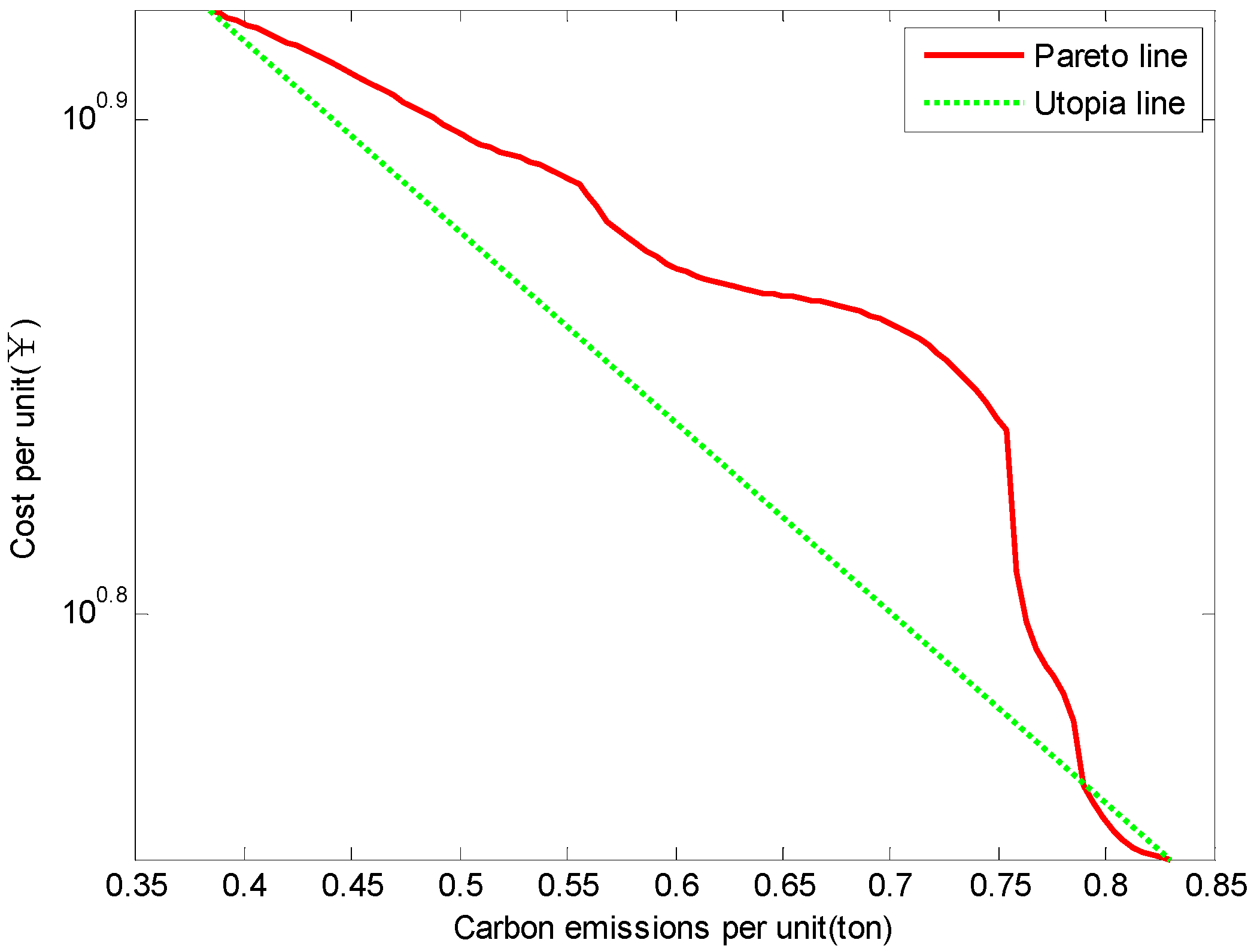
6.2. Numerical Analysis

According to the above data and the approach used to solve the question in Section 5, the trade-off between cost and carbon emissions can be shown as Figure 4.The result provides decision makers with decidedly indifferent choices. In conclusion, all the points on the Pareto line are the solutions, but the managers themselves cannot directly decide. If CEBs are incorporated, the optimal solution is unique (Figure 5). Clearly, revenue first increases and then decreases with increasing carbon emissions. The increasing gradient is greater than the decreasing gradient. This result illustrates that a proper carbon reduction policy can improve corporate revenue, but excessive carbon reduction activities would have a negative impact. Figure 5 shows that the maximum attainable revenue is ¥601,230,000. The optimal configuration can be shown as follows: The location decision is to open Cangzhou, Jinan, and Zhengzhou. The routing decision is divided into two parts. (i) As regards the routing from plants to warehouses, the first decision is that Daqing serves Cangzhou and Jinan, while Fushun serves Zhengzhou. (ii) Considering transportation from warehouses to retailers, the routing schedule of the Cangzhou warehouse is Cangzhou-Tianjin-Beijing-Baoding-Cangzhou-Shijiazhuang-Taiyuan-Cangzhou. The routing schedule for the Jinan warehouse is Jinan-Liaocheng-Linyi-Qingdao-Jinan, and the routing schedule for the Zhengzhou warehouse is Zhengzhou-Xinyang-Yuncheng-Zhengzhou. The order quantities of the three warehouses are 4792, 3156 and 2834 tons, respectively.

We are interested in how CEBs affect companies’ decision making. As we know, CEBs mainly affect demand. The effect of consumers’ environmental preference on demand for products with different carbon emissions is shown in Figure 6. We vary the CEBs from 1 to 1.8 and obtain a series of demand vs. carbon emissions. Clearly, the curves move from left to right as the coefficient increases from 1 to 1.8, which implies that with the same carbon emission levels, larger CEBs lead to greater demand. This is due to the fact that when consumers pay closer attention to environmental protection, enterprises are more likely to take actions that will improve their environmental protection levels. Then, consumers with greater environmental awareness will buy more products from those enterprises with superior eco-friendly operations. This is a virtuous cycle. However, the marginal cost of implementing environmental improvements increases by degrees. As we know, the ultimate goal of enterprise management is to maximize benefits. Similarly, we adjust the carbon emissions variable to analyze the effect of CEBs on revenue (Figure 7). Clearly, revenue increases as the CEBs move from 1 to 1.8. However, the degree of revenue growth is clearly slower than the increasing CEBs. That is to say, the initial improvement brought about by the CEBs greatly affects the operation of supply chain enterprises, but this effect will weaken because of the high costs associated with further reductions of carbon emissions.

We assume that product pricing is a function of carbon emissions. However, it is not a hard and absolute fact that pricing is the single, key factor. Our analysis (Figure 8) shows that higher prices generate greater revenue. What is important is that the higher the price of a product, the bigger the revenue will be obtained with lower carbon emissions. This illustrates that a higher price for green products can stimulate a reduction in carbon emissions, but that higher price can also curb product demand (Figure 9). Clearly, product pricing is increasing with a reduction in carbon emissions. When the price increases, the product demand decreases. In this case, the consumer’s willingness to pay is the most important factor. Hence, the enterprise should encourage consumers to improve their CEBs, and pay closer attention to purchasing green products.

6.3. Managerial Insights

In the current business climate, enterprises and consumers have gradually come to recognize the importance of environmental protection. Both businesses and consumers are more inclined to make an effort to reduce carbon emissions. In particular, consumers with greater environmental awareness are happy to pay a premium price for low carbon emission products. This willingness, which is based on increased environmental awareness, provides an opportunity for logistics enterprises. Our study is consistent with the work of Liu et al. [8], which found that, with consumers’ greater environmental awareness, more of them are willing to pay higher prices for low carbon emission products. In turn, the enterprises that produce those products can earn greater revenue.

In addition, the companies that produce low carbon emissions should also make a concerted marketing effort to shift consumers’ traditional purchasing decision criteria and transform those buyers into a group with a preference for low carbon emission products and services. This study indicates that the returns can be substantial if consumers who are currently not interested in purchasing environmentally friendly products make even a little progress. Moreover, the results show that low carbon emission operations cost more than the operations that do not consider carbon emissions. However, when the CEBs are positive, an optimal degree of carbon reduction will maximize revenue. Sadly, the unavoidable fact is that most consumers loathe paying to pay premium prices for low carbon emission products. If enterprises are going to implement sustainable decisions, they must be certain of CEBs.

7. Conclusions

This paper discussed the effects of consumer environmental behaviors (CEBs) on the design of a sustainable supply chain. CEBs not only affect consumers’ willingness to pay premium prices for low carbon emission products, but also the overall demand for low carbon emission products. We introduced a sustainable supply chain network model based on the joint optimization of location, routing and inventory, taking carbon emissions into consideration. The distinguishing feature of our model is its consideration of the CEBs, which affect both carbon emission decisions and product demand.

First, a multi-objective model is constructed, which provides a trade-off between costs and carbon emissions. The MOPSO algorithm is used to solve the model, and then a Pareto optimal set can be obtained. After that, we model the revenue function based on the Pareto solutions. In the computational experiments, we test the model by the data from the Northeast Chemical Sales Company of CNPC. We first obtain the Pareto optimal curve, which provides a portfolio of configurations for decision makers. Then, we can use the same technique to obtain the revenue curves from different carbon emissions. Hence, the unique optimal revenue levels and the relevant decisions can be acquired. Finally, the sensitivity of the case study was analyzed. We are interested in the effects of CEBs on the demand and revenue in a three-level supply chain. The results show that more positive CEBs result in greater demand and higher revenue. We also observe that the pricing of low carbon operations is critical. Therefore, enterprises should make marketing efforts to strengthen consumers’ environmental preferences. Companies should support their claims to consumers and ensure the degree of CEBs before implementing their carbon emission reduction policies.

Further research is required to determine more specific factors pertaining to CEBs in a supply chain (e.g., the decision makers’ appetite for risk, the expectations of market development and the effects of government intervention via carbon emission reduction policies and legislation), so that the model will be more adaptive to real-life scenarios.

References

1. Hufbauer, G.C.; Charnovitz, S.; Kim, J. Global Warming and the World Trading System; Peterson Institute for International Economics: Washington, DC, USA, 2009. [Google Scholar]
2. Chistra, K. In search of the green consumers: A perceptual study. J. Serv. Res. 2007, 7, 173–191. [Google Scholar]
3. Conrad, K. Price competition and product differentiation when consumers care for the environment. Environ. Resour. Econ. 2005, 31, 1–19. [Google Scholar] [CrossRef]
4. Laroche, M.; Bergeron, J.; Barbaro-Forleo, G. Targeting consumers who are willing to pay more for environmentally friendly products. J. Consum. Market. 2001, 18, 503–520. [Google Scholar] [CrossRef]
5. Moon, W.; Florkowski, W.J.; Brückner, B.; Schonhof, I. Willing to pay for environmental practices: Implications for eco-labeling. Land Econ. 2002, 78, 88–102. [Google Scholar] [CrossRef]
6. Ghosh, D.; Shah, J. A comparative analysis of greening policies across supply chain structures. Int. J. Prod. Econ. 2012, 135, 568–583. [Google Scholar] [CrossRef]
7. Gil-Moltó, M.J.; Varvarigos, D. Emission taxes and the adoption of cleaner technologies: The case of environmentally conscious consumers. Resour. Energy Econ. 2013, 35, 486–504. [Google Scholar] [CrossRef]
8. Liu, Z.L.; Anderson, T.D.; Cruz, J.M. Consumer environmental awareness and competition in two-stage supply chains. Eur. J. Oper. Res. 2012, 218, 602–613. [Google Scholar] [CrossRef]
9. Elhedhli, S.; Merrick, R. Green supply chain network design to reduce carbon emissions. Transp. Res. Part D 2012, 17, 370–379. [Google Scholar] [CrossRef]
10. Paksoy, T.; Özceylan, E.; Weber, G.W.; Barsoum, N.; Weber, G.W.; Vasant, P. A multi objective model for optimization of a green supply chain network. Glob. J. Technol. Optim. 2011, 2, 84–96. [Google Scholar]
11. Paksoy, T.; Özceylan, E. Environmentally conscious optimization of supply chain networks. J. Oper. Res. Soc. 2013, 65, 855–872. [Google Scholar] [CrossRef]
12. Benjaafar, S.; Li, Y.; Daskin, M. Carbon footprint and the management of supply chains: Insights from simple models. IEEE Trans. Autom. Sci. Eng. 2013, 10, 99–115. [Google Scholar] [CrossRef]
13. Kim, N.S.; Janic, M.; Van Wee, B. Trade-off between carbon dioxide emissions and logistics costs based on multiobjective optimization. Transp. Res. Rec. J. Transp. Res. Board 2009, 2139, 107–116. [Google Scholar] [CrossRef]
14. Wang, F.; Lai, X.F.; Shi, N. A multi-objective optimization for green supply chain network design. Decis. Support Syst. 2011, 51, 262–269. [Google Scholar] [CrossRef]
15. Chaabane, A.; Ramudhin, A.; Paquet, M. Design of sustainable supply chains under the emission trading scheme. Int. J. Prod. Econ. 2012, 135, 37–49. [Google Scholar] [CrossRef]
16. Chen, X.; Benjaafar, S.; Elomri, A. The carbon-constrained EOQ. Oper. Res. Lett. 2013, 41, 172–179. [Google Scholar] [CrossRef]
17. Babiker, M.H.; Criqui, P.; Ellerman, A.D.; Reilly, J.M.; Viguier, L.L. Assessing the impact of carbon tax differentiation in the European Union. Environ. Model. Assess. 2003, 8, 187–197. [Google Scholar] [CrossRef]
18. Jabali, O.; Woensel, T.V.; de Kok, A.G. Analysis of Travel Times and CO2 Emissions in Time-Dependent Vehicle Routing. Prod. Oper. Manag. 2012, 21, 1060–1074. [Google Scholar] [CrossRef]
19. Nagy, G.; Salhi, S. Location-routing: Issues, models and methods. Eur. J. Oper. Res. 2007, 177, 649–672. [Google Scholar] [CrossRef]
20. Dror, M.; Ball, M. Inventory/routing: Reduction from an annual to a short-period problem. Naval Res. Logist. (NRL) 1987, 34, 891–905. [Google Scholar] [CrossRef]
21. Shen, Z.J.M.; Coullard, C.; Daskin, M.S. A joint location-inventory model. Transp. Sci. 2003, 37, 40–55. [Google Scholar] [CrossRef]
22. AhmadiJavid, A.; Azad, N. Incorporating location, routing and inventory decisions in supply chain network design. Transp. Res. Part E Logist. Transp. Rev. 2010, 46, 582–597. [Google Scholar] [CrossRef]
23. Ahmadi-Javid, A.; Seddighi, A.H. A location-routing-inventory model for designing multisource distribution networks. Eng. Optim. 2012, 44, 637–656. [Google Scholar] [CrossRef]
24. Hua, G.W.; Cheng, T.C.E.; Wang, S.Y. Managing carbon footprints in inventory management. Int. J. Prod. Econ. 2011, 132, 178–185. [Google Scholar] [CrossRef]
25. Kroes, J.; Subramanian, R.; Subramanyam, R. Operational compliance levers, environmental performance, and firm performance under cap and trade regulation. Manuf. Serv. Oper. Manag. 2012, 14, 186–201. [Google Scholar] [CrossRef]
26. Diabat, A.; David, S. A Carbon-Capped Supply Chain Network Problem. In Proceedings of the IEEE International Conference on Industrial Engineering and Engineering Management, Hong Kong, China, 8–11 December 2009; IEEE press: Piscataway, NJ, USA, 2010; pp. 523–527. [Google Scholar]
27. Wygonik, E.; GooDChild, A. Evaluating CO2 emissions, cost and service quality trade-offs in an urban delivery system case study. IATSS Res. 2011, 35, 7–15. [Google Scholar] [CrossRef]
28. Thøgersen, J. Promoting Green Consumer Behavior with Eco-Labels. In New Tools for Environmental Protection: Education, Information, and Voluntary Measures; Dietz, T., Stern, P., Eds.; National Academy Press: Washington, DC, USA, 2002; pp. 83–104. [Google Scholar]
29. Young, W.; Hwang, K.; McDonald, S.; Oates, C.J. Sustainable consumption: Green consumer behaviour when purchasing products. Sustain. Dev. 2010, 18, 20–31. [Google Scholar] [CrossRef]
30. Vanclay, J.K.; Shortiss, J.; Aulsebrook, A.; Gillespie, A.M.; Howell, B.C.; Johanni, R.; Maher, M.J.; Mitchell, K.M. Customer response to carbon labeling of groceries. J. Consum. Policy 2011, 34, 153–160. [Google Scholar] [CrossRef]
31. Tang, C.S.; Zhou, S. Research advances in environmentally and socially sustainable operations. Eur. J. Oper. Res. 2012, 223, 585–594. [Google Scholar] [CrossRef]
32. Desrochers, M.; Laporte, G. Improvements and extensions to the Miller-Tucker-Zemlin subtour elimination constraints. Oper. Res. Lett. 1991, 10, 27–36. [Google Scholar] [CrossRef]
33. Kennedy, J.; Eberhart, R. Particle swarm optimization. In Proceedings of the IEEE International Conference on Neural Networks, Perth, Australia, 27 November–1 December 1995; pp. 1942–1948.
34. Shankar, B.L.; Basavarajappa, S.; Chen, J.C.; Kadadevaramath, R.S. Location and allocation decisions for multi-echelon supply chain network–a multi-objective evolutionary approach. Expert Syst. Appl. 2013, 40, 551–562. [Google Scholar] [CrossRef]
35. Everson, R.M.; Fieldsend, J.E.; Singh, S. Full Elite Sets for Multi-Objective Optimisation. In Adaptive Computing in Design and Manufacture V; Springer: London, UK, 2002; pp. 343–354. [Google Scholar]
36. Ling, H.F.; Zhou, X.Z.; Jiang, X.L.; Xiao, Y.H. Improved constrained multi-objective particle optimization algorithm. J. Comput. Appl. 2012, 32, 1320–1324. [Google Scholar]
Figure 1. The framework of supply chain network.
Sustainability 08 00211 g001
Figure 2. The mapping relationship of archive A and population S.
Sustainability 08 00211 g002
Figure 3. The network of two plants, five potential warehouses and 14 retailers.
Sustainability 08 00211 g003
Figure 4. Pareto optimal curve between cost and carbon emissions.
Sustainability 08 00211 g004
Figure 5. The relationship between carbon emissions and revenue.
Sustainability 08 00211 g005
Figure 6. The demand in different consumer environmental preferences varying with carbon emissions.
Sustainability 08 00211 g006
Figure 7. The revenue in different consumer environmental preferences varying with carbon emissions.
Sustainability 08 00211 g007
Figure 8. The revenue vs. carbon emissions in different product pricing.
Sustainability 08 00211 g008
Figure 9. The relationship between product pricing -carbon emissions, and product pricing-product demand.
Sustainability 08 00211 g009