Assessing Collective Measures in Rural Policy: The Effect of Minimum Participation Rules on the Distribution of Benefits from Irrigation Infrastructure

Abstract

Despite the increasing interest from both policy makers and scholars in the collective management of natural resources in the rural sector, the literature has not covered many aspects of the incentives targeting collective actors. In this article, we analyze how embedding minimum participation rules in rural policies affect the distribution of benefits of a group of players that cooperate. The article applies the Shapley Value and the Nash–Harsanyi solution, two of the key solutions of cooperative game theory, to an incentive scheme in Emilia-Romagna (Italy) to support the construction of collective reservoirs for irrigation water. Results show that rules on the minimum storage capacity and on the minimum number of users affect the benefit distribution in opposite directions. The main conclusion of the article is that minimum participation rules should be carefully designed if welfare distribution is an issue. However, further studies are required to have a comprehensive assessment of minimum participation rules within rural policies.

1. Introduction

The sustainability of the agricultural sector partially depends on the conservation of key natural resources, such as biodiversity, ecosystem services and freshwater, that are threatened by the increasing demand for food [1]. For this reason, in recent decades, the focus of agricultural policies has shifted from the pure support of market prices/production/income to include the management of these resources. Traditionally, the measures promoting environmentally friendly practices in agriculture have been largely based on support to individual farms [2,3]. However, this is considered less and less effective in achieving ecosystem/resource-related objectives. A collective approach has been advocated for policies focusing on the interconnection between agriculture and natural resource management given that environmental protection exhibits different degrees of non-rivalry and non-excludability and it is characterized by thresholds and spatial factors that require the coordination of farmers [4].

This topic is increasingly relevant for the design of agri-environmental policies, especially in the European Union (EU), which is envisioning and promoting the coordination among farms of the application of environmental efforts, both in the first pillar (for the collective compliance of the “greening” constraints associated with the CAP direct payments) (Art. 46, Regulation (EU) No. 1307/2013 of the European Parliament and of the Council) and in the second pillar (suggesting to Member States to provide higher payments when groups of farmers are jointly the recipients of agri-environment-climate payments) (Paragraph 22 and Art. 28, Regulation (EU) No. 1305/2013 of the European Parliament and of the Council). Often, the strategy to embed a collective approach in rural policies is to link the incentives to collective conditionality constraints such as Minimum Participation Rule (MPR). A MPR sets a minimum number of farmers or a minimum extent of land contracted above which a premium is allocated to the participants. Some examples clarify this. In some specific areas of France, incentives for the implementation of clustered buffer strips (aimed at reducing the impact of non-point source pollution on surface water) are conditional on the contracting of at least 60% of the target area [5]. Such a MPR is set at the landscape level and de facto imposes the cooperation of a number of farmers to be met. In Emilia-Romagna (E-R), Italy, the Rural Development Plan (RDP), one of the key agricultural policies in the EU, provides incentives for the construction of rainwater harvesting reservoirs with the environmental goal of decreasing the pressure on groundwater resources. This measure defines two eligibility constraints for the potential projects: one on the minimum size of the reservoirs (50,000 m³), and the other on the minimum number of participating farmers (20) (in E-R, in the 2000–2006 RDP such a measure is described in the Axes 3, measure 3q; in the 2007–2013 RDP such a financial scheme is granted by Axes 1, measure 125; and, in the 2014–2020 RDP this type of support is introduced in the measure M04—Investments in physical assets (art 17), sub-measure 4.3, operation 4.3 B).

In the literature, incentives for the spatial coordination of environmental efforts have been advocated by Parkhurst et al. [6] who define an “agglomeration bonus”, namely a subsidy for environmental conservation in which a premium is granted when plots of land devoted to conservation are adjacent to each other. The literature has further analyzed the topic, identifying other agglomeration incentive schemes, such as agglomeration payments [7], or multi-round auctions [8]. The analysis of these types of incentives has often been based on Non-Cooperative Game Theory (NCGT) and tested empirically through experimental games. These experiments show that, for example, communication [6], experience in “playing” [9], the availability of information regarding others’ choices [10], and smaller groups [11] are all elements that facilitate the coordination of players. Mathematical models are often employed to assess the degree of effectiveness of these types of incentives in plausible but simplified setups [5,12]. Most of the mathematical models include the land allocation decision in a global optimization objective function [13,14], in some cases allowing side-payments [7]. Concerning water management, “ambient” mechanisms, developed to reduce non-point source pollution from agricultural landscapes, have been proposed [15]. Research on the management of irrigation water (quantity) has traditionally addressed the collective dimension given the large amount of agents involved, the frequent lack of centralized coordination [16], and the economies of scale in infrastructure development [17,18]. However, this literature has mostly overlooked at the relationship and the interactions between policy and agents, at least explicitly [19].

Even though the topic has been the subject of a greater number of analyses in recent years, many aspects of agglomeration incentives in rural policies have not been addressed by the scientific literature. For instance, the distribution of benefits is considered an important issue to take into account in the design of the voluntary approach to the management of natural resources [20] but has not been the subject of much analysis. More generally, equity and distributional considerations are considered relevant determinants of the success of cooperation and the coordination of agents [21,22]. This has been recognized by the agglomeration bonus literature that acknowledges but, to the best of our knowledge, does not analyze, the importance of the bargaining process and the resulting distribution of benefits [7].

Given these considerations, in this article we assess the distribution of the benefits generated by an agglomeration incentive scheme. More specifically, we assess how the imposition of different MPRs affects the bargaining power of farmers, and as a result, the likely individual shares of the policy subsidy. To study this issue, we use a Cooperative Game Theory (CGT) approach with transferable utility. In particular we numerically compute the Shapley Value (SV) and the Nash–Harsanyi (NH) solution of the cooperative environment affected by collective incentives and we assess how these solutions vary with changes in the MPR levels. Our analysis is numerically applied to a simple case that exemplifies the implementation of measure 125 of the RDP 2007–2013 of E-R, which provides financial support for the construction of collective reservoirs. The financial support is conditional on the minimum size of reservoir capacity (q-rule hereinafter) and on the minimum number of participating farms (n-rule hereinafter) [23].

CGT solutions explicitly focus on the distribution of the worth of a joint venture, and thus seem to properly address the questions raised in this study. A vast literature has applied CGT solutions to issues related to the cooperative management of water and environmental resources [24,25], including, for example, the allocation of costs or benefits from water treatments [26,27], droughts management [28], groundwater [29] and multi-reservoir systems [30]. These studies have shed some lights on the implications and on the stability of cooperation without the complexity and difficulty of specifying in details the players’ strategies as in a NCGT framework. The SV gives a normative and unique solution to the problem of allocating the worth of a group of agents working together, a coalition, by defining a share that is based on the average marginal contribution of each player to each possible coalition. For these reasons, the SV can be interpreted as the expected value of cooperating [31] and thus it seems an appropriate proxy for the likely distributional impact of the policy schemes here analyzed. The NH solution attributes the share of the grand coalition worth depending on the disagreement points that are defined by the non-cooperative outcomes. The SV captures more comprehensively the whole implications of different MPR than the NH solution. Nevertheless, by interpreting them as different distributional institutions, the comparison of the two solutions gives insights on the effect of MPR across different preferences and/or hypothesis on benefit distribution [29].

Moreover, it is to be noted that, given that these solutions can only be applied to cases in which the profitability of cooperation has already been verified, we overlook the problem of mechanism design, which would be a prior step. In keeping with this, we take as exogenously given the policy rules that we investigate here. Additional elements of discussions on these issues are presented later in the article.

Our article adds the CGT perspective to the literature on agglomeration incentives and rural policies, providing some insights into the distribution of the expected gains from cooperation generated by a policy program. We acknowledge that most of the analyses on agglomeration bonus are based on NCGT, but we believe that the use of CGT in the context under analysis in this article is justifiable in the light of the considerable amount of anecdotal evidence available regarding communication among players and (de-facto) binding agreements—the two underlying assumptions of CGT—among farmers in a rural community. Moreover, in this context, we also provide an initial assessment of how MPRs can change the structure of the game and subsequently some consideration can be made on how to design such rules for environmental policies in rural landscapes. Models of coalition formation have suggested that a MPRs are potentially helpful coordination devices to solve the free-rider problem associated with the provision of a global public good such as climate change mitigation [32,33,34,35]. However, to the best of our knowledge, their effect on the bargaining power have been overlooked, even though it seems that preferences on MPR levels could also depend on this [36].

The article is structured as follows. In the next section, we describe the theoretical CGT foundation of the current analysis and the numerical application. The paper continues by presenting the results. Finally, the discussion and the conclusion are in the last two sections.

2. Methods

2.1. The Caracteristic Function in a Reservoir Construction Game and the Effect of of the q-Rule and of the n-Rule

Assume that a number of heterogeneous farms i, where i = 1, …, n need to build reservoirs in order to make water available for irrigation. Further imagine that the farms in question can pool together their resources to build the reservoir, and that they can gain financial support from the regional administration if MPRs are met. When all the farms cooperate together we have the “grand coalition” defined by N, the set that includes all i farms. Farms can also arrange themselves in coalitions, sub-groups of the entire population; call S the set of the feasible coalitions in the game, with s indicating a given coalition ($s\subseteq N$).

By cooperating, any coalition gains a value v(s), which is the “characteristic function” of the game. The usual assumption on the characteristic function is its superadditivity, namely that the full cooperation among all the farmers leads to the highest aggregated profits. Assuming we have two disjoint coalition s and t ($s\cap t=\varnothing$), both belonging to S, superadditivity is defined by: $v\left(s\cup t\right)\ge v\left(s\right)+v\left(t\right)$.

Assume in our specific case, that the characteristic function is defined by the following maximization problem, namely each coalition must solve:

$$\mathrm{Max}[R-(1-\alpha P)k\left(Q_s\right)]$$

(1)

s.t.

$$Q_s={\displaystyle \sum _{i\in s}{Q}_i}$$

(2)

$$R={\displaystyle \sum _{i\in s}{R}^i\left(Q_i\right)}$$

(3)

$$P=\{\begin{array}{l}0 \mathrm{if} Q_s<q^t\\ 1 \mathrm{if} Q_s\ge q^t\end{array}$$

(4)

R is the sum of the individual revenues of the members of coalition s as a function of the water quantity (Q_s) given by the reservoir. We assume that individual revenues are given by quadratic functions in the water quantity, so that the inverse demand functions are linear. k(Q_s) is the cost of the reservoir construction exhibiting economies of scale (k’(Q_s) > 0 and k’’(Q_s) < 0) thus satisfying the super-additive assumption. P is a binary variable that indicates whether the coalition participates or not in the RDP. $\alpha \in \left[0,1\right]$ is the share of the costs covered by the RDP. Finally, Equation (4) defines the MPR as a q-rule that links the financial support to the (exogenously determined) minimum size (q^t) of the reservoir. The coalition has to maximize the difference between the sum of the individual benefits generated by irrigation, and the costs of constructing a (possibly) collective reservoir, which thus depends on the aggregate amount of water requested.

The problem entails a binary variable and cannot be solved analytically. There are two choice variables: the water quantity demanded by the farms (the reservoir size), and whether or not it is profitable to participate in the RDP given the threshold q^t and the share of the costs covered by the RDP. To analyse the problem we first assess the optimal reservoir size and profits with and without the financial support, and second we assess the effect of the q-rule. These results are then used to define the characteristic function.

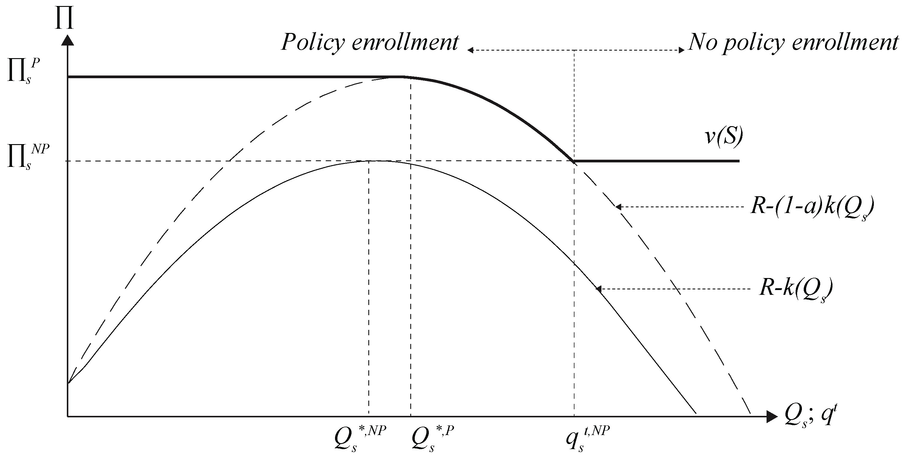
In case there is no public support (α = 0), the first order conditions are given by the point of intersection of the aggregated marginal revenue function and the cost function: $R_{Q_s}=K_{Q_s}$. The result is the optimal reservoir size in the absence of the financial support (superscript “NP”) Q_s^*,NP, and the associated profits Π_s^NP(Q_s^*,NP). q^t = 0, the first order conditions are similar to the previous case: $R_{Q_s}=\alpha K_{Q_s}$, leading to the optimal reservoir size Q_s^*,P and coalition profits Π_s^P(Q_s^*,P). Given the assumptions on the shapes of the functions we have that Q_s^*,P > Q_s^*,NP and Π_s^P(Q_s^*,P) > Π_s^NP(Q_s^*,NP).

The introduction of the q-rule entails that the characteristic function could assume three values, depending on the level of the q-rule relative to the optimal reservoir sizes. First, as long as the q-rule is not binding, Q_s^*,P ≥ q^t, the problem is trivial. The coalition participates in the RDP, the q-rule has no effect, and the value that coalition s obtains is Π_s^P(Q_s^*,P). If we increase q^t above Q_s^*,P, the size of the reservoir is given by the q-rule level and the resulting profits are Π_s^P(q^t). However, the coalition still participates in the RDP as long as q^t ≤ q_s^t,NP, where q_s^t,NP is the level in the q-rule at which Π_s^P(q^t) = Π_s^NP(Q_s^*,NP). Finally, for q^t level higher than q_s^t,NP, the coalition obtains the profits in the absence of the policy support: Π_s^NP(Q_s^*,NP). Accordingly, the characteristic function of the game when a q-rule applies is:

$$v\left(s\right)=\{\begin{array}{l}{\mathsf{\Pi }}_s^P\left(Q_s^{*P}\right) \mathrm{if} Q_s^{*P}\ge q^t\\ {\mathsf{\Pi }}_s^P\left(q^t\right) \mathrm{if} Q_s^{*P}<q^t\mathrm{and} {\mathsf{\Pi }}_s^{P,t}\ge {\mathsf{\Pi }}_s^{NP}\\ {\mathsf{\Pi }}_s^{NP}\left(Q_s^{*NP}\right) \mathrm{if} Q_s^{*P}<q^t\mathrm{and} {\mathsf{\Pi }}_s^{P,t}<{\mathsf{\Pi }}_s^{NP}\end{array}$$

(5)

The theoretical analysis previously described is summarized graphically in Figure 1. Profits with and without financial support increase up to the level of the optimal reservoir size, and then decrease. The characteristic function is constant as long as the q-rule is lower than the optimal reservoir size when costs are partially covered by the regional administration. Then it decreases up to the level of profits without the financial support, which set a floor on the characteristic function level.

The introduction of an n-rule, by setting a threshold on the minimum number of participants (n^t) into the game would add another constraint that changes Equation (4) into:

$$P=\{\begin{array}{l}0 \mathrm{if} Q_s<q^t \mathrm{or} \left|s\right|<n^t\\ 1 \mathrm{if} Q_s\ge q^t \mathrm{and} \left|s\right|\ge n^t\end{array}$$

(6)

where |s| is the cardinality of the set s, i.e., the number of members in the coalition. The characteristic function thus becomes:

$$v\left(s\right)=\{\begin{array}{l}{\mathsf{\Pi }}_s^P\left(Q_s^{*P}\right) \mathrm{if} Q_s^{*,P}\ge q^t\mathrm{and} \left|s\right|\ge n^t\\ {\mathsf{\Pi }}_s^P\left(q^t\right) \mathrm{if} Q_s^{*,P}<q^t \mathrm{and} {\mathsf{\Pi }}_s^P\ge {\mathsf{\Pi }}_s^{NP}\mathrm{and} \left|s\right|\ge n^t\\ {\mathsf{\Pi }}_s^{NP}\left(Q_s^{*NP}\right) \mathrm{if} Q_s^{*,P}<q^t \mathrm{and} {\mathsf{\Pi }}_s^P<{\mathsf{\Pi }}_s^{NP}\mathrm{and} \left|s\right|\ge n^t\\ {\mathsf{\Pi }}_s^{NP}\left(Q_s^{*NP}\right) \mathrm{if} \left|s\right|<n^t \end{array}$$

(7)

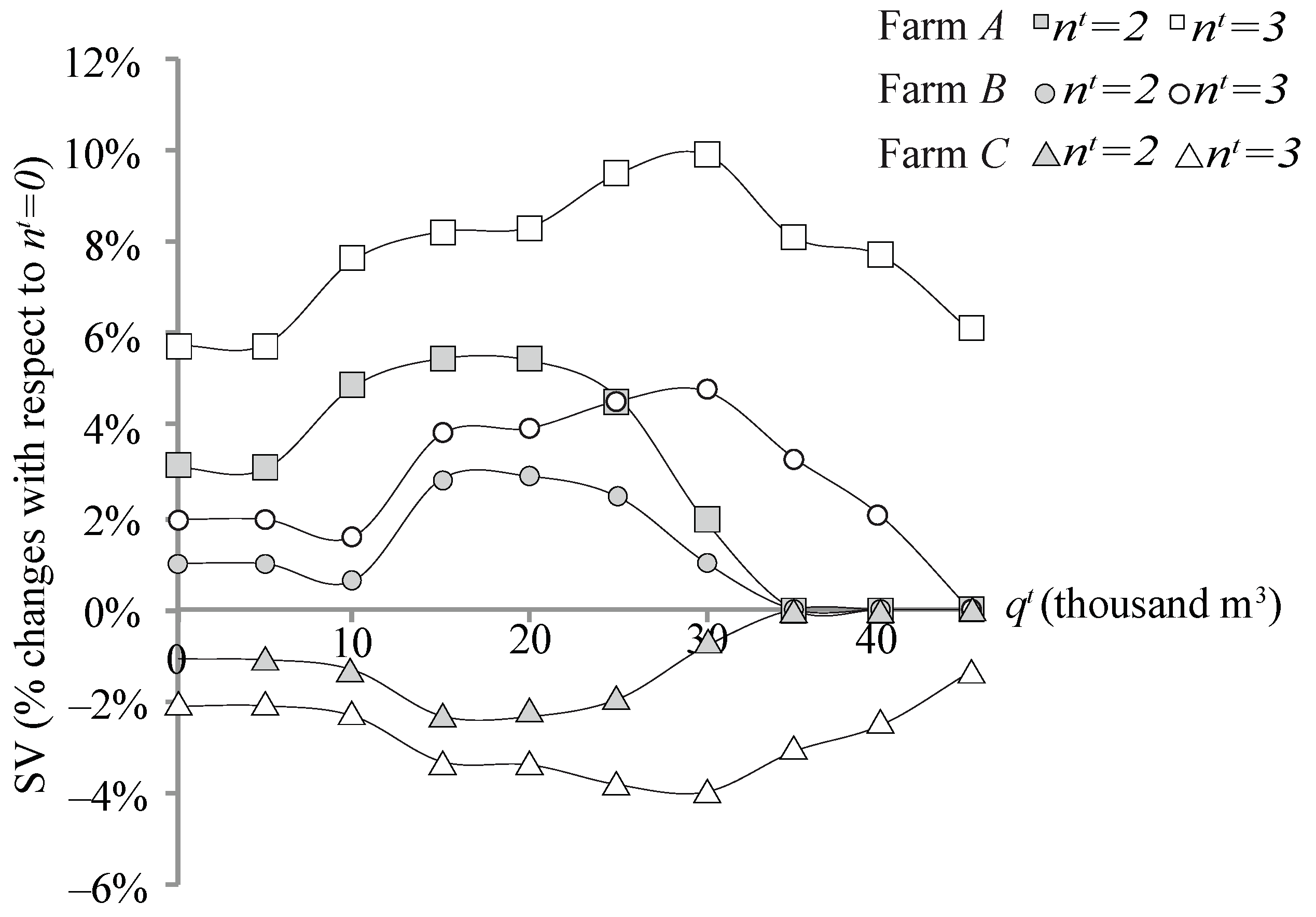
The MPRs not only affect the characteristic function of a single decisional unit but they change the structure of the cooperative game. First, they increase the attractiveness of the full cooperation with respect to the other possible arrangements. For example, assume that there are three players (I = A,B,C) having different revenue function shapes with Q_A^*,P < Q_B^*,P. In addition, recall that given the shape of the cost function we have Q_A^*,P < Q_B^*,P < Q_(A,B)^*,P. As long as q^t ≤ Q_A^*,P, Q_B^*,P the gains from cooperation, are simply given by the economies of scale due to the cost function, since any coalition benefit from the financial support. Further increases in the threshold add to the economies of scale the fact that for singleton coalitions it is relatively more difficult to access the financial support, whereas it is still feasible for the two-players coalition. Cooperation becomes more and more attractive because the q-rule imposes costs on the smaller coalition. This continues as long as q_A^t,NP, q_B^t,NP ≤ q^t < q_(A,B)^t,NP, namely when only singleton coalitions do not enroll in the policy, and thus the gains from cooperation are at the their highest level.

Second, if farms are heterogeneous, MPR affects the game asymmetrically. The increases in the gains from cooperation are first due to the decrease in the profits of player A, and then due to the decrease in the profits of player B. This asymmetry influences the relative bargaining power within the grand coalition. Consider the two q-rule levels q^t1 < q^t2 < Q_N^*P, which do not affect the worth of the grand coalition. Imagine a coalition (A,C) for which v(A,C) = Π_s^P(Q_s^*,P) given a fixed q^t1 and v(A,C) = Π_s^NP(Q_s^*,NP) given a fixed q^t2. The increase in the threshold reduces the potential worth of (A,C), and increases the relative gains from full cooperation. Moreover, the bargaining power of player B is thus greater now, since coalition (A,C) has now a lower opportunity cost of fully cooperating with player B (or, in other terms, cooperation for them becomes relatively more attractive).

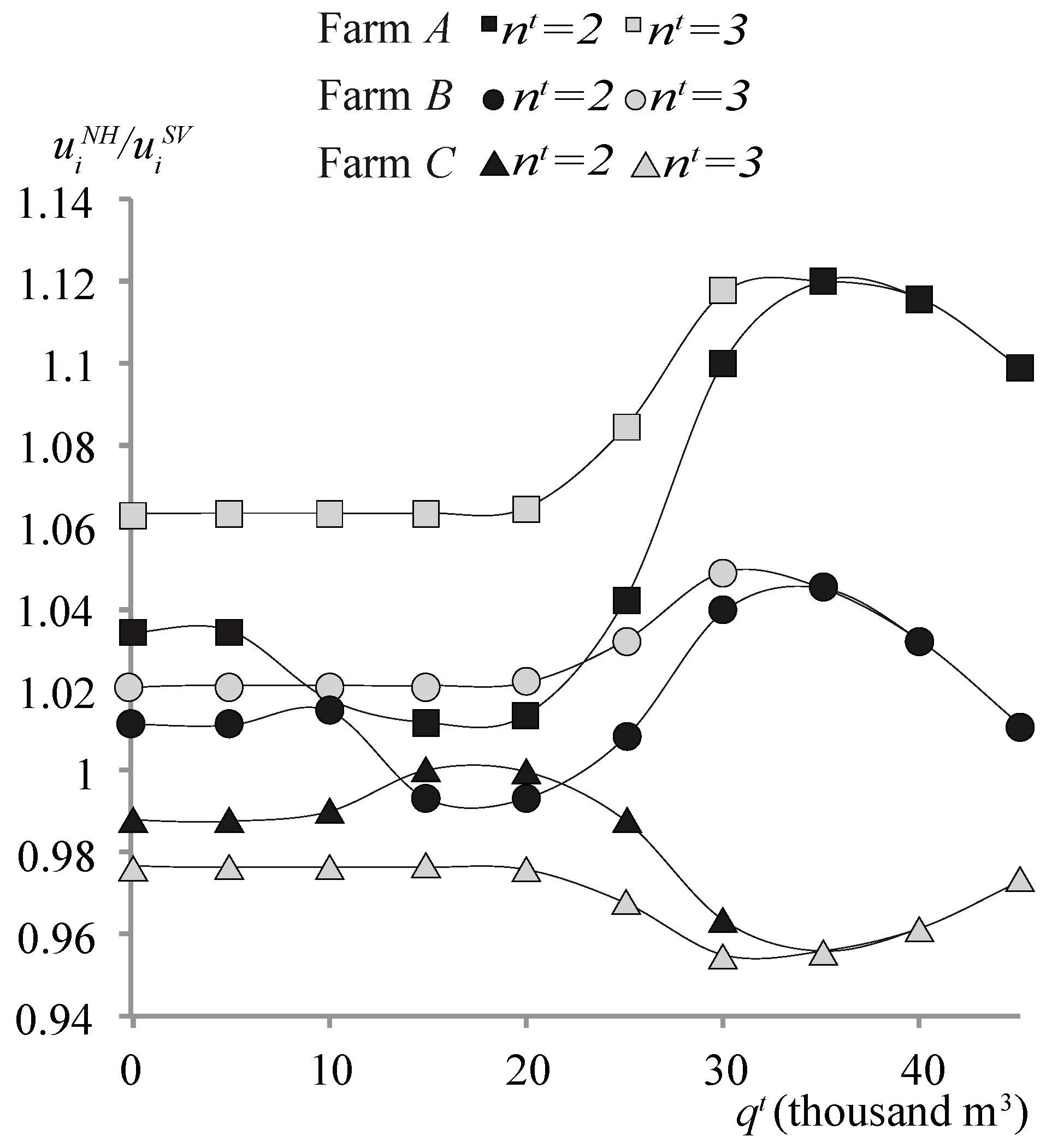
2.2. Shapley Value and Nash–Harsanyi Solution

How to share the worth of cooperation in such a way that all of the i players enter the grand coalition? Call u_i^* the worth attributed to the ith agent in the full cooperation setup. The “core” of a cooperative game defines the set of rationally acceptable solutions u_i^* and it is defined by the following system of inequalities [37]:

$${\displaystyle \sum _{i\in s}{u}_i^{*}}\ge v\left(s\right)\hspace{1em}\hspace{1em}\forall s\in S,S\subseteq N$$

(8)

$${\displaystyle \sum _{i\in N}{u}_i^{*}}=v\left(N\right)$$

(9)

Equation (8) is the rationality constraints, which state that a solution, a share of the grand coalition worth, must be such that all the people cooperating gain more in the full cooperative agreement than in any possible sub-groups, including the singleton coalitions when players act non-cooperatively. Equation (9) is the efficiency constraint, stating that the entire wealth of the grand coalition is to be shared among the players. The non-existence of a solution to the system of Inequalities (8) and (9) defines an “empty” core. In turn, a game characterized by an empty core is considered to be unstable, since there is no possibility to share the grand coalition worth in such a way that all players find such an arrangement profitable. In this condition, most likely the grand coalition will not form. In addition, if it does not meet the core conditions, a sharing rule will not be accepted by the whole set of players.

The SV is a unique solution that in the case of convex games undoubtedly satisfies the previous inequalities, and is thus in the core [38,39]:

$$u_i^{*}=u_i^{SV}={\displaystyle \sum _{\begin{array}{l}S\subseteq N\\ i\in S\end{array}}\frac{\left(n-\left|s\right|\right)!\left(\left|s\right|-1\right)}{n!}}\left[v\left(s\right)-v\left(s-\left\{i\right\}\right)\right]$$

(10)

where for ∀i ∈ N, |s| is the number of members in the coalitions, and n is the total number of participants in the game [29]. Equation (10) states that the worth attributed to the ith player through the SV is given by its average marginal contribution to any possible grouping of the players. The marginal contribution of any player i is defined by the expression v(s) − v(s − {i}), which indicates that is given by the value obtained by the coalition minus the value obtained by the coalition when player i is not a member of it. The greater the contribution of a player is to a coalition, the greater his or her final share of the grand coalition is worth.

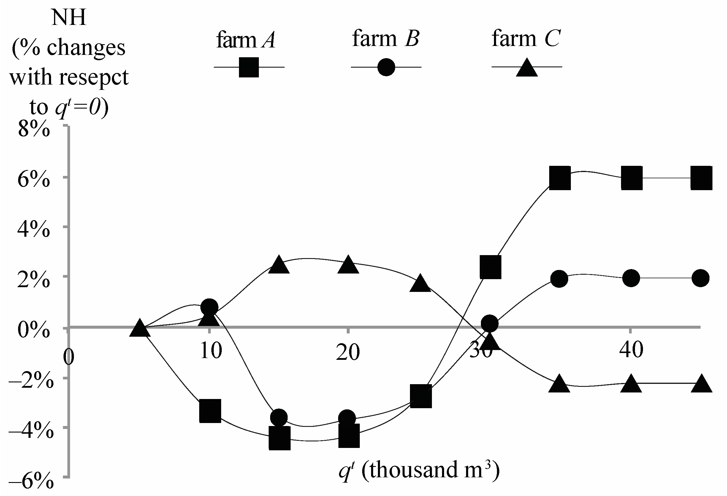
An example clarifies what is the marginal contribution of a player, and how could be potentially affected by changes in MPR levels. Imagine we have three farmers (i = A,B,C) that as singletons have profits of v(A) = 10, v(B) = 20 and v(C) = 30. Further consider that v(A,B) = 40. Imagine there are policy incentives linked to a MPR level of three farmers (n^t = 3), so that by both pooling resources and receiving the subsidy they obtain: v(A,B,C) = 100. In this situation, the marginal contribution of player C to the coalition (A,B,C) is given by: v(A,B,C) − v(A,B) = 60. Now imagine that there is an alteration in the MPR level so that the n-rule becomes n^t = 2, and v(A,B)’ = 65. The marginal contribution of C is now v(A,B,C) − v(A,B)’ = 35. Everything else constant, in the second situation the bargaining power of player C is greatly reduced, even though neither the aggregated final payoff, nor his singleton payoff has changed. MPR thus might increase the gap between the cooperative arrangements that meet the requirements of the MPR and the smaller groupings that are administratively excluded, resulting in changes in the bargaining power of the players that ultimately affect the distribution of the benefits.

The NH solution is the extension to the n-person game of the Nash solution to the bargaining problem. The solution is given by the result of the following maximization problem:

$$\max {\displaystyle \prod _i^n\left(u_i^{NH}-v\left(i\right)\right)}$$

(11)

subject to the core conditions (Equations (8) and (9)). Equation (11) indicates that the NH solution is obtained by maximizing the product of the gains from cooperation with respect to the non-cooperative outcomes. Thus, the NH is relatively more sensible to changes in the in singleton coalitions’ worth than to changes in the value obtained by e.g., 2-players coalitions.

These solutions are often compared in terms of the stability of the wealth allocation. There are a number of methods to compare the different CGT solutions in terms of stability. One of these is Propensity To Disrupt index (PTD) [40], that has been often used as an indicator of the stability of cooperation [29]. The PTD for player i measures the ratio between how much the players other than i would lose if i leaves the grand coalition and the loss that i would face. The lower the PTD, the higher player i gains from cooperating with respect to the other players and so the relatively higher are his or her incentives to cooperate. Mathematically, the PTD is defined by:

$$PT{D}_i=\frac{{\displaystyle \sum _{j\ne i}{u}_j^{*}-v\left(N-\left\{i\right\}\right)}}{u_i^{*}-v\left(i\right)}$$

(12)

In the next section we provide an example that more closely resembles the problem of the collective reservoir and the subsidy schemes, to which we apply the SV and the NH solution.

2.3. Numerical Application

Here we apply the previous analysis to a numerical example for illustrative purposes, parameterizing the model as much as possible on actual data while maintaining the tractability and intelligibility of the game. The example is based on secondary data taken from the E-R region, from an area where irrigation water is managed by the Consorzio di Bonifica della Romagna Occidentale (CBRO), a local Water User Association. The choice of the area is due to the high rate of successful applications to the measure 125 of the regional RDP, since eight out of sixteen applications in E-R were submitted by group of farmers through the CBRO.

Assume there are three farms (i = A,B,C) that are characterized by different levels of water productivity. As a numerical example, we take the revenue function from a mathematical programming model elaborated by Viaggi et al. [41]. The model is a farm profit maximization problem where land allocation and irrigation are some of the decision variables, and water availability is one of the key constraints. The original model is applied to an area within the CBRO territory where farms are grouped through a cluster analysis, where the discriminants are farm size and share of land allocated to crop types [41]. In this paper, we use three of the five original farm clusters: cluster 2 (farm A), cluster 3 (farm B), and cluster 4 (farm C). All three of the farm clusters are characterized by a relatively high share of land allocated to permanent crops (highly dependent on water availability) and they represent the most frequent farm typologies in the area. Here the results from [41] are simplified by using a quadratic interpolation (to be consistent with the previous analysis) of the gross margin results generated by a sensitivity analysis on water availability, not considering the costs of the water provision:

$$R^i=l_i\left({\eta }_i{q}_i^2+{\beta }_i{q}_i+{\gamma }_i\right)$$

(13)

where q_i is the water quantity per hectare, and total water used by the farm is $Q_i=l_i{q}_i$. The farm specific parameters are listed in

Table 1. Farm specific parameters.

Revenue Function Parameters	Farm A	Farm B	Farm C
η	−0.0002	−0.0005	−0.0006
β	1.2017	1.1498	1.1803
γ	680.22	747.05	817.76
l	3.76 ha	12.54 ha	32.59 ha

. The three farms are relatively heterogeneous in terms of both land availability, and water productivity. Farm A is the smallest and the one with the steepest revenue function.

Restricting focus to a three-player game ensures the tractability of the problem and the comprehensiveness of the results. However, there is a clear trade-off between tractability and (i) the ability of the model to represent the heterogeneity of the composition of the farmers in the group; and (ii) the degree of discrepancy with respect to the actual number of users in each reservoir, which are in a range of 20–50 [42].

The construction costs of the reservoir are given by the annualization (λ = 0.05) of the investment costs derived from the following function: 140(Q_s)^0.641. The cost function was formulated in collaboration with officials of the CBRO, and represents the interpolation of the costs assessment of a number of planned reservoirs with different capacity levels. Moreover, we introduce running costs (c) to account for electricity and management. We assume that running costs are dependent on the coalition size and account for economies of scale in management, technical choices, and more likely water scarcity for the smaller reservoirs. According to CBRO officials, these are key factors to be considered when decisions on building reservoirs are made. In the absence of more precise functions, marginal running costs are assumed to be dependent on the number of reservoirs user: c = 0.45 if |s| = 1, c = 0.30 if |s| = 2, and c = 0.15 if |s| = 3. We do not address the problem of the connection costs among the farms and the reservoir as it is not possible to properly represent the complexity of such an issue (spatial elements, congestion costs) in a three-player game. However, CBRO officials report that these costs can be higher than 50% of total costs for existing reservoirs. The drawback is thus that the model certainly overestimates the reservoir capacity. The final cost function is $K\left(Q_s\right)=\lambda \cdot 140{\left(Q_s\right)}^{0.641}+c{Q}_s$.

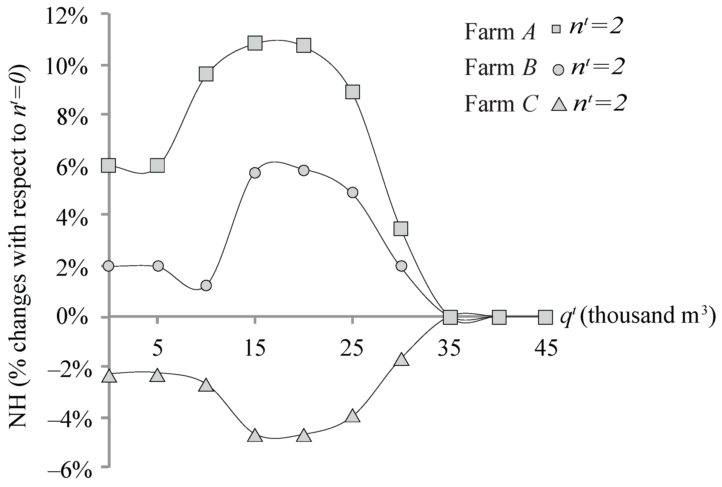
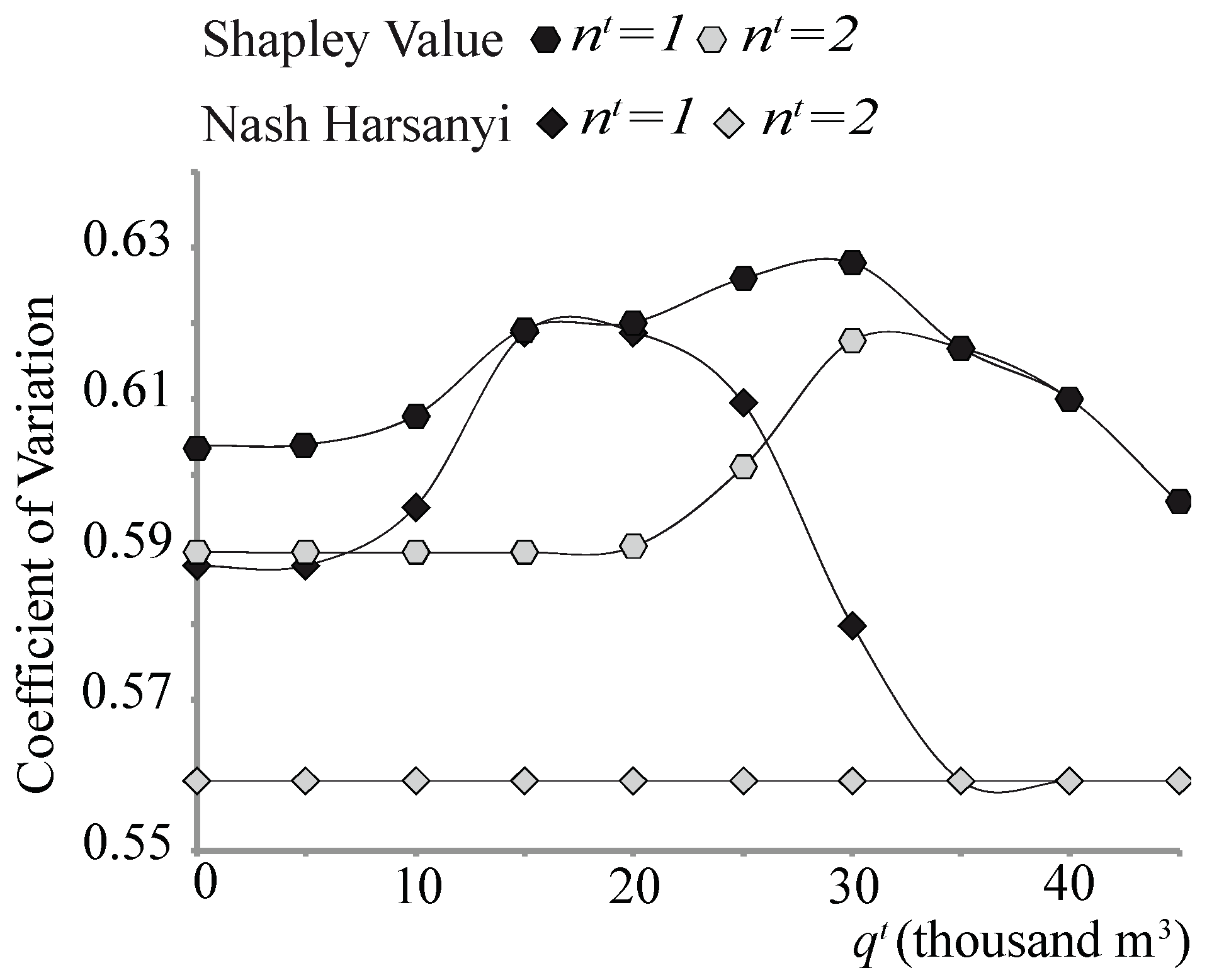
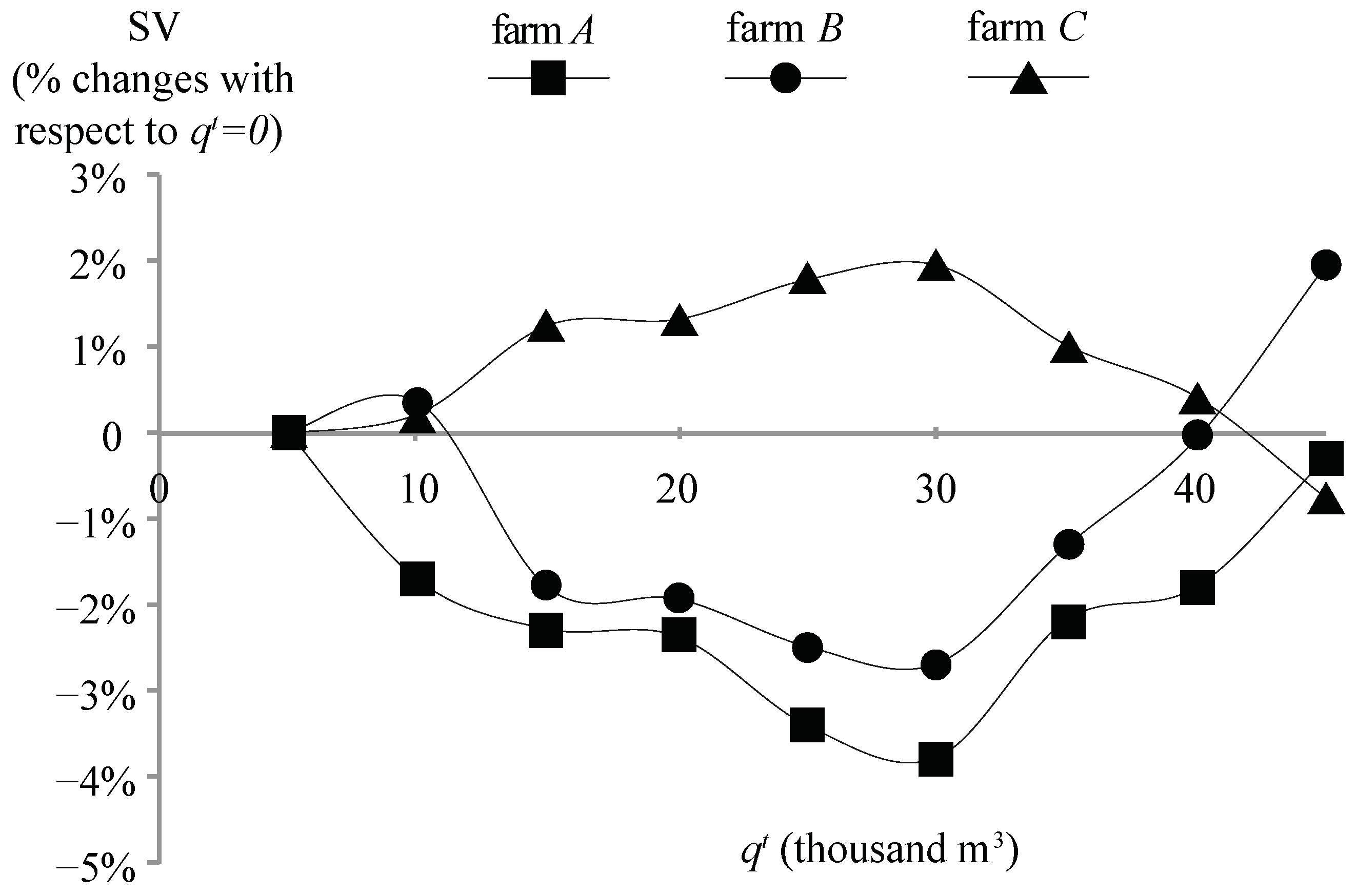
We explore the characteristic function, the SV and the NH solution for different levels of q-rules and n-rules (n^t = 1, n^t = 2, n^t = 3) in case of α = 0.7. Once again, the tractability of the results imposes a simplification and scaling down of the MPRs applied for the example described here (n^t = 0, and q^t = 50,000 m³ are the actual levels).

3. Results

3.1. Effect of MPR on the Characteristic Function

Table 2. Profits with (Π_s^P(Q_s^*,P)) and without financial support (Π_A^NP(Q_A^*,NP)), q-rule threshold (q_s^t,NP) and optimal reservoir size in case of financial support (Q_s^*,P).

Coalition	ΠsP(Qs*,P) (€)	ΠsNP(Qs*,NP) (€)	qst,NP (m3)	Qs*,P (m3)
(A)	4951	3610	12,082	7009
(B)	12,170	10,622	15,048	8754
(C)	33,693	30,996	32,344	20,150
(A,B)	19,126	16,585	28,893	18,261
(A,C)	41,938	38,328	47,523	31,185
(B,C)	49,386	45,620	50,680	33,292
(A,B,C)	62,306	57,438	70,992	49,036

presents the elements, for each coalition, that the previous section has highlighted to be relevant in the assessment of the effect of the MPR on the characteristic function (Π_s^P(Q_s^*,P), Π_s^NP(Q_s^*,NP), q_s^t,NP and Q_s^*,P). As it is clear from the Table 2, the size of the farms plays a key role given that the q-rule is in absolute values. Relatively low q-rule levels make it profitable for (A) and (B) as singletons to withdraw from the policy, and does likewise to the bigger coalitions and (C). Above q^t = 32,344 any singleton coalition do not enroll in the RDP and the policy benefits are only ensured by joining bigger coalitions. This continues up to q^t = 49,036, after which the q-rule also imposes costs on the grand coalition’s worth and thus restricts the benefit from fully cooperating. Above q^t = 70,992, even the grand coalition withdraws from the policy, and the only gains from joining the grand coalition are due to the economies of scale of the original game, which sets a floor for the characteristic function of the game (hence further values are not analyzed).

Table 2 shows the two effects, highlighted in the previous section, that raising the threshold could have on the game. First, it increases the attractiveness of the full cooperative arrangement, since the gains from cooperation in our game are due to the economies of scale and to the enrolment in the policy. For example, at q^t = 0, the added value of cooperation is ${\mathsf{\Pi }}_n^P\left(Q_n^{*P}\right)-{\displaystyle \sum _i{\mathsf{\Pi }}_i^P\left(Q_i^{*P}\right)}=11,492$, whereas for 32,344 < q^t ≤ 49,036 it becomes ${\mathsf{\Pi }}_n^P\left(Q_n^{*P}\right)-{\displaystyle \sum _i{\mathsf{\Pi }}_i^{NP}\left(Q_i^{*NP}\right)}=17,078$. Keeping q^t = 0, the same result is reached by increasing the n-rule, passing from n^t = 1 to n^t = 2. Second, it asymmetrically affects the marginal contribution of the players, and thus their bargaining power. For instance, passing from q^t = 0 to q^t = 8000 entails a reduction in the marginal contribution of farm B to coalition (AB) from Π_(A,B)^P(Q_(A,B)^*,P) − Π_A^P(Q_A^*,P) = 14,157 to Π_(A,B)^P(Q_(A,B)^*,P) − Π_A^NP(Q_A^*,NP) = 15,516, whereas any other marginal contribution remains constant.

3.2. Shapley Value

The entire relative changes in SVs across the different policy schemes and threshold levels are due to relative changes in the opportunity costs of the arrangements other (smaller) than the grand coalition. Recall that for q-rule levels q^t ≤ Q_N^*,P = 49,036, the threshold does not affect the grand coalition’s worth, and any change in the SV is only due to the costs imposed by the q-rule on the smaller arrangements.

In the absence of any policy (α = 0), the SV for the three players are u_A^SV = 7358, u_B^SV = 14,511, and u_C^SV = 35,569, representing respectively 13%, 25% and 62% of the grand coalition worth. Introducing the financial support of the policy, and in the absence of any MPR (q^t = 0 and n^t = 1), the SV allocates benefits as follow: u_A^SV = 8490, u_B^S = 15,824, and u_C^SV = 37,991. These values represent respectively 14%, 25% and 61% of the grand coalition worth. Not surprisingly, in both cases, farm C (i.e., the biggest one) gains the highest share, followed by farm B and finally farm A. Consider also that the financial support increases profits by 15% for farm A, 9% for farm B and 7% for farm C, with respect to the no-policy situation. How the MPRs affect the distribution of the benefits in the SV case?

First we present the results when the financial support is dependent on the size of the reservoirs but not on the number of the farmers that are connected. We thus analyse the effect on the SV of the q-rule (q^t ≥ 0), when no n-rule applies (n^t = 1). To observe the effect of the q-rule, in Figure 2 we depict how, by increasing the q-rule level, the SV changes in percentage terms with respect to q^t = 0 (absolute values are reported in the

Table A1. Shapley Value for any Minimum Participation Rule level.

	nt = 1			nt = 2			nt = 3
Farm	A	B	C	A	B	C	A	B	C
qt = 0	8490	15,824	37,991	8751	15,981	37,574	8981	16,133	37,192
qt = 5000	8490	15,824	37,991	8751	15,981	37,574	8981	16,133	37,192
qt = 10,000	8346	15,881	38,079	8751	15,981	37,574	8981	16,133	37,192
qt = 15,000	8298	15,539	38,469	8751	15,981	37,574	8981	16,133	37,192
qt = 20,000	8290	15,520	38,495	8740	15,970	37,596	8981	16,133	37,192
qt = 25,000	8202	15,432	38,671	8581	15,811	37,914	8981	16,133	37,192
qt = 30,000	8171	15,401	38,734	8327	15,557	38,421	8981	16,133	37,192
qt = 35,000	8307	15617	38,382	8307	15,617	38,382	8981	16,133	37,192
qt = 40,000	8339	15,814	38,153	8339	15,814	38,153	8981	16,133	37,192
qt = 45,000	8466	16,133	37,707	8466	16,133	37,707	8981	16,133	37,192

). Both farms A and B decrease their SV as long as q^t ≤ 30,000, up to, respectively, −2% and −4% with respect to q^t = 0. The opposite occurs for farm C that increases its SV by a maximum of 2%. Using the notation of the previous section, an increase in the q-rule level rapidly imposes to farm A and B a quantity greater than the coalition optimal reservoir size, thus imposing a cost on the coalitions (q^t > Q_s^*,P). This entails that their opportunity costs of not joining the grand coalition decrease rapidly so that farm C can legitimately claim a progressively larger share of the grand coalition’s worth. Above q^t = 30,000, singletons (A) and (B) and coalition (A,B) are not affected by increases to the q-rule. Within the same range of q^t levels, (C) withdraws from the policy, and its only chance to obtain financial support is now by joining with the other farms. Its opportunity costs are thus decreased, as is its share of the grand coalition’s worth.

Note that these changes are greater if we use the no-policy situation as a reference point. With respect to a counter-world where there is no policy, for farm A the gains from the policy range from a 15% increase at q^t = 0, down to an 11% when q^t = 30,000, and up again to a maximum of 21% when q^t = 50,000. Farms B and C are less affected by the q-rule: gains are in the range of 6% and 11% for farm B, and between 6% and 9% for farm C.

Second, we describe the effect of the n-rule. We compare the SV of the three players when the financial support is not conditional on the number of the users of the reservoirs (n^t = 1, the previous case), with a situation where such a support is granted if at least two (n^t = 2) and three farms (n^t = 3) are connected to the reservoir. When n^t = 3, the q-rule has no effect on the distribution of the benefits. Figure 3 depicts for the three farms the result in the SV at n^t = 2 and n^t = 3 in percentage terms with respect to n^t = 1, for any q-rule levels. The results show that the n-rule has a different and neater effect on the SV. First, the higher the n-rule, the higher the SV of players A and B, and the lower the share of player C. Second, the n-rule has a greater effect than the q-rule. While the maximum change in the SV due to the q-rule was around 2%–4%, the n-rule n^t = 3 increases the SV of farm A up to almost 10%, up to 5% for farm B, and it decreases the SV up to −4% for farm C. Size matters relatively less, since the big players cannot have access to the greater advantage of cooperation granted by access to the RDP and need the cooperation of the smaller farms. In other terms, with the q-rule even singleton players can obtain the financial support, and get Π_s^P, while in case of the n-rule they cannot obtain more than Π_s^NP, which is lower.

3.3. Nash–Harsanyi Solution

In the case of no policy support, the NH solution would attribute €7680 to farm A (13%), 14,692 to farm B (26%) and 35,065 to farm C (61%). In the case of the policy financial support, and no MPR, the shares of the grand coalition worth are 8782 for farm A (14%), 16,001 (26%) for farm B and 37,523 (60%) for farm C. These shares represent an increase of 14% for farm A, 9% for farm B and 7% for farm C with respect to the no policy scenario.

Similar to Figure 2, Figure 4 presents the effect of the MPR on the NH solution, depicting the change in percentage terms with respect to q^t = 0 (absolute values are reported in the

Table A2. Nash–Harsanyi solution for any Minimum Participation Rule level.

	nt = 1			nt = 2			nt = 3
Farm	A	B	C	A	B	C	A	B	C
qt = 0	8782	16,001	37,524	9303	16,315	36,688	9303	16,315	36,688
qt = 5000	8782	16,000	37,524	9303	16,315	36,688	9303	16,315	36,688
qt = 10,000	8492	16,115	37,699	9303	16,315	36,688	9303	16,315	36,688
qt = 15,000	8396	15,431	38,479	9303	16,315	36,688	9303	16,315	36,688
qt = 20,000	8404	15,416	38,486	9303	16,315	36,688	9303	16,315	36,688
qt = 25,000	8546	15,558	38,203	9303	16,315	36,688	9303	16,315	36,688
qt = 30,000	8990	16,002	37,314	9303	16,315	36,688	9303	16,315	36,688
qt = 35,000	9303	16,315	36,688	9303	16,315	36,688	9303	16,315	36,688
qt = 40,000	9303	16,315	36,688	9303	16,315	36,688	9303	16,315	36,688
qt = 45,000	9303	16,315	36,688	9303	16,315	36,688	9303	16,315	36,688

). The NH solution is mostly affected by the value of the non-cooperative outcome, and this is reflected in the graph. Up to q^t = 20,000 the value of v(A) and v(B) decreases up to Π_s^NP(Q_s^*,NP) level, while v(C) remain constant. As a consequence, the NH solutions gives an increasing share of the grand coalition worth to farm C. Above q^t = 20,000, the q-rule negatively affect farm C too, and, keeping in mind that v(A,B,C) remain constant, a progressively higher share of the grand coalition worth is assigned to the players A and B. This marks a difference between the SV and NH solution, since the highest gains for player C comes at bigger q-rule levels. At q^t = 35,000 the q-rule is so high that also player C finds no longer profitable to participate in the RDP, and the NH no longer is affected by the q-rule.

The effect of the n-rule is substantially different on the NH than on the SV. Here the n-rule affects the distribution of the benefit when passing from n^t = 1 to n^t = 2, but there is no change in passing from n^t = 2 to n^t = 3. Again, the reason behind this result is that the NH solution is more sensible to changes in the non-cooperative outcome than to changes in the other coalition worth. Passing form n^t = 1 to n^t = 2 entails that the singleton coalitions are no longer eligible for the financial support and their characteristic functions becomes Π_s^NP(Q_s^*,NP), but further changes are not absorbed by the NH solution. As it is clear from Figure 5 the difference in NH solution with respect to the SV are not qualitatively different if we only consider the changes from n^t = 1 to n^t = 2. Farm A and farm B gain from the greater n^t values, whereas farm C is the one suffering from the change. However, changes are more ample than in the SV.

3.4. Comparison of the Solutions

Figure 6 below depicts the NH solution as a share of the SV for the q-rule levels and for n^t = 1 and n^t = 2. Since at n^t = 3 the q-rule is irrelevant, such a result is not depicted in the graph. However, the ratio in such a case is 1.03, 1.01 and 0.98 for respectively farm A, farm B and farm C, at any level of the q-rule. First, these results shows how farm A and B have a greater share of the grand coalition worth in a NH institutional setting than in the SV setting irrespectively on the MPR levels. If the distribution institutional arrangement would be endogenously chosen, e.g., by voting, the NH arrangement would be the one that emerges. Second, the differences between the solutions increase with the q-rule levels. The reason is that the major changes in the q-rule are not accounted by the NH solution.

An additional point of comparison is the heterogeneity in the distribution. As it was noted in the introduction, distributional considerations are regarded to be important when cooperation is at stake. In Figure 7 we depict the coefficient of variation of the benefits distributed by the SV and by the NH solution for different q-rule and n-rule levels. The results on n^t = 3 are not depicted because in any case they are not affected by the q-rule. At n^t = 3, the coefficient of variation for the SV is 0.58, while in case of the NH solution is 0.56 for any q-rule level. First, as it is clear from the figure, the SV entails a more heterogeneous benefit distribution than the NH solution for any q-rule level. Second, the effect of the q-rule on the heterogeneity of the SV is less pronounced than in the NH solution. The SV coefficient of variation passes from a maximum of 0.63 to a minimum of 0.60, while the coefficient of variation of the NH solution shows a maximum of 0.62 to a minimum of 0.56. This is again due to the fact that in the NH solution changes in the non-cooperative outcome are not buffered by the marginal contributions to the bigger coalitions as in the case of the SV.

The final mean of comparison that we use is the Propensity To Disrupt index (PTD) [40]. All the results of the PTD are in the Appendix B (

Table B1. Propensity to disrupt index in the case of the Shapley Value, for any Minimum Participation Rule level.

	nt = 1			nt = 2			nt = 3
Farm	A	B	C	A	B	C	A	B	C
qt = 0	1.25	1.24	1.21	0.81	0.82	0.85	1.43	1.42	1.38
qt = 5000	1.25	1.24	1.21	0.81	0.82	0.85	1.43	1.42	1.38
qt = 10,000	1.19	1.19	1.16	0.81	0.82	0.85	1.43	1.42	1.38
qt = 15,000	0.99	0.99	0.99	0.81	0.82	0.85	1.43	1.42	1.38
qt = 20,000	0.99	0.99	0.99	0.81	0.82	0.86	1.43	1.42	1.38
qt = 25,000	1.03	1.03	1.02	0.87	0.88	0.91	1.43	1.42	1.38
qt = 30,000	1.04	1.04	1.03	0.97	0.97	0.98	1.43	1.42	1.38
qt = 35,000	0.99	0.99	0.99	0.99	0.99	0.99	1.43	1.42	1.38
qt = 40,000	1.09	1.08	1.06	1.09	1.08	1.06	1.43	1.42	1.38
qt = 45,000	1.27	1.24	1.19	1.27	1.24	1.19	1.43	1.42	1.38

and

Table B2. Propensity to disrupt index in the case of the Nash–Harsanyi solution, for any Minimum Participation Rule level.

	nt = 1			nt = 2			nt = 3
Farm	A	B	C	A	B	C	A	B	C
qt = 0	1.08	1.14	1.48	0.64	0.71	1.14	1.3	1.35	1.59
qt = 5000	1.08	1.14	1.48	0.64	0.71	1.14	1.3	1.35	1.59
qt = 10,000	1.11	1.06	1.37	0.64	0.71	1.14	1.3	1.35	1.59
qt = 15,000	0.95	1.03	0.98	0.64	0.71	1.14	1.3	1.35	1.59
qt = 20,000	0.94	1.03	0.99	0.64	0.71	1.15	1.3	1.35	1.59
qt = 25,000	0.89	0.97	1.22	0.64	0.71	1.32	1.3	1.35	1.59
qt = 30,000	0.73	0.81	1.56	0.64	0.71	1.59	1.3	1.35	1.59
qt = 35,000	0.64	0.75	1.59	0.64	0.75	1.59	1.3	1.35	1.59
qt = 40,000	0.73	0.9	1.59	0.73	0.9	1.59	1.3	1.35	1.59
qt = 45,000	0.94	1.17	1.59	0.94	1.17	1.59	1.3	1.35	1.59

). Analysing the results show that players A and B have always a greater PTD in the case of the SV benefit allocation than in the NH solution. The opposite occurs for player C. These findings further underpin that the NH solution would be the most preferred institutional setup in this game. Furthermore, they show that increasing the n-rule causes an increase in the PTD for all the players and for both distributional institutions. The effect of the q-rule is more ambiguous and it depends on the n-rule level.

4. Discussion

The results show the effect of MPRs on the potential sharing of the worth of a common project. Such rules affect the opportunity costs of joining a grand coalition, so that the bargaining power of the players is also affected. Setting relatively high MPR reduces the value of the sub-optimal coalitions, which can no longer access public financial support, and it increases the relative advantages of full cooperation in the grand coalition. We assess and compare two solutions developed by CGT under different MPR: the SV and the NH solution. The SV distributes the worth of the grand coalition taking into account all of the possible arrangements other than the grand coalition that can emerge, reporting a value that reflects the contributions that each player provides to the coalitions. The NH distributes benefits according to the disagreement points, which are in turn defined by the non-cooperative outcomes. The MPRs that we analyzed here affect differently the opportunity costs of participating in the grand coalition, and thus influence the bargaining power of the players, which is ultimately reflected in changes to the SV and in the NH, and in different effects on the two solutions.

The two rules (based on a minimum total volume and a minimum number of players) affect the SV and the NH of the players in different ways. An initial increase in the q-rule tends to depress the shares of the grand coalition worth of the smaller players and to benefit the bigger players as long as the smaller players are the ones that are relatively more affected by the cost imposed by the q-rule. Further increases re-equilibrate the distribution after the big farm withdraws from the policy and its access to the financial support is granted only by cooperating. This result is not qualitatively different across the two solutions. However, the effects of changes in the q-rule are relatively greater in the NH than in the SV solution. On the other hand, a rule on the number of players tends to favour the smaller players since the participation in the RDP is granted only by coordinating with other players and the financial support is a major component of the benefits of cooperation. Moreover, such a rule exhibits a qualitatively different effect across the two solutions. Being relatively more sensible to changes in the value of singletons, the NH does no address the changes in the n-rule when n^t is raised above n^t = 2.

The comparison of the two solutions shows that in any case the NH would be the preferred distributional institution. Two out of three players gain more in the NH than in the SV. Moreover, both the heterogeneity in the distribution and the PTD are lower in the NH than in the SV, indicating that a NH solution is likely to be more stable. This result however should be best tested empirically through, e.g., laboratory experiments aimed at assessing both the importance and the preference on distributional issues. Such findings would also be important for the identification of the most appropriate proxy for a proper ex-ante assessment of the distributional impact of the introduction of MPR in agricultural policies.

The results are difficult to compare with other studies, except for those straightforward, such as the effect of policy support on optimal water quantity and profits. However, our results seem to be qualitatively in line with the findings of Kesternich, even though his analysis is at the country level [36]. The author, using online surveys, investigates the preferences of delegates to the United Nations Framework Convention on the level of MPR regarding both the minimum number of participating countries, and minimum amount of emission reductions. Results indicate that preferences are rather different according to country of origin. Small countries prefer rather high MPRs that thus can garner them greater bargaining power. On the other hand, larger economies favor the formation of smaller coalitions (relatively low MPR) and relatively high emission reduction levels.

The results and the methodology are subject to a number of limitations.

First, the results are numerically obtained, and thus they are partially dependent on the choices of the parameters. For instance, reducing the heterogeneity in the farms would also result in a less heterogeneous shares and MPR effects. On the other hand, increasing the steepness of the water demand function would stress the effect of increasing the MPR. The effect of the n-rule on the NH solution is likely to be relatively robust, even though major changes in the characteristic functions might affect it through the core conditions.

Second, results are to be carefully interpreted since MPR and policies are to be assessed also, of course, in terms of efficiency and/or effectiveness. Recall that CGT solutions can only be applied after the superadditivity of the game have been verified. Since we were mainly interested in the distributional effect of the conditional constraints of the policy, we took a relatively simple example, where cooperation is always profitable. However, it is not difficult to imagine that joint costs in water development projects are affected by interactions across players other than the economies of scale. Transaction costs associated with bargaining and network costs are both elements that are dependent on the number of players involved in the project. The inclusion of these types of costs in the model could change the effect of the policy scheme on the profitability of the cooperative arrangements (in the CGT approach, that would be a change in the characteristic function of the game). More precisely, in the presence of relatively high club costs, the financial support of the RDP might actually be needed to make cooperation profitable. On the other hand, setting a low participation threshold would again hamper cooperation, making the singleton arrangement relatively more profitable. The main outcome of a better analysis of the characteristic function would likely reduce the range of parameter levels within which the game is superadditive, and the CGT solutions can be applied.

Moreover, we analyzed a three-player game to have a clear understanding of the main issues that are the subject of the research. CGT analyses are not easy to scale up given their combinatorial nature and the need of clear and detailed information on the characteristic function of the game for all of the possible coalitions. On the other hand methodological advancements have been employed to apply CGT to larger systems, such as the meaningful spatial aggregation of units [43], the modification of the SV to account for different probabilities of coalition formation [44], and sampling approaches to compute the SV [45].

On the other hand, the findings of this analysis can be extended to the different agglomeration incentives that have been proposed to create clusters of protected areas. Even though the structure of the problem is different, CGT solutions seem indeed to be some of the proper tools for the assessment of the distributional effects of agglomeration incentives since it can easily address some of the key features of these. For instance, spatial elements (soil quality, spatial relations among players) can be easily introduced. It is worth imagining, for instance the assessment of different thresholds on the extent of the land contracted: in a Ricardian framework an increase in the size-rule would imply that better land is contracted in the context of conservation programs, thus increasing the opportunity costs of participating in the project, and ultimately affecting the SV of the players. Alternatively, say for instance that farm B is in between farm A and C, which do not share borders with each other. Clearly, any agglomeration incentives could not be accessed by players A and C without the presence of player B, so that its bargaining power is higher, and it can legitimately claim a relatively greater share of grand coalition worth.

5. Conclusions

In this paper, we study how collective conditionality constraints that determine the eligibility of a water reservoir development project using public financial support affect the allocation of the worth generated by the project in two different distributional institutions (the SV and the NH). The results show that setting MPR affects the relative profitability of alternative cooperative arrangements and the individual profitability of joining different arrangements. It also affects the individual and collective gains from financial support through policy. More precisely, first, the results indicate that MPRs tend to increase the attractiveness of cooperation. Second, they suggest that setting a minimum size rule tends to increase the power of the larger players, whereas setting a minimum number of players relatively favors more the smaller players. However, a more comprehensive assessment of MPR must include detailed assessment of the costs strictly associated with coordinated efforts (i.e., transaction costs, pipeline network), and it is needed to better define the characteristic functions of the game (the maximum worth a coalition can obtain), and in particular the actual effects of low threshold levels.

The results are subject to a number of limitations and the assumptions related to the specific problems analyzed herein, and mostly important the reliance on simplified data. In spite of this, some of the findings can likely be extended to a broad class of issues related to biodiversity and environmental conservation actions in RDPs—in particular when the incentive structure encourages cooperation among players to achieve better environmental/ecological outcomes. Moreover, it seems that the CGT solutions can be successfully applied to the analysis of agglomeration incentive policies. Future research could be dedicated to the application of cooperative game theory to these types of policies, addressing the associated specificities (i.e., spatial relations, and Ricardian models).

Altogether, collective conditionality of rural policy appears to be gaining in importance, and CGT shows promise as a tool for the assessment of distributional effects and as a support to policy design.

References

1. Velten, S.; Leventon, J.; Jager, N.; Newig, J. What Is Sustainable Agriculture? A Systematic Review. Sustainability 2015, 7, 7833–7865. [Google Scholar] [CrossRef]
2. Lefebvre, M.; Espinosa, M.; Gomez y Paloma, S.; Paracchini, M.L.; Piorr, A.; Zasada, I. Agricultural landscapes as multi-scale public good and the role of the Common Agricultural Policy. J. Environ. Plan. Manag. 2014. [Google Scholar] [CrossRef]
3. Baylis, K.; Peplow, S.; Rausser, G.; Simon, L. Agri-environmental policies in the EU and United States: A comparison. Ecol. Econ. 2008, 65, 753–764. [Google Scholar] [CrossRef]
4. Organisation for Economic Co-Operation and Development (OECD). Providing Agri-Environmental Public Goods through Collective Action; OECD: Paris, France, 2013. [Google Scholar]
5. Dupraz, P.; Latouche, K.; Turpin, N. Threshold effect and co-ordination of agri-environmental efforts. J. Environ. Plan. Manag. 2009, 52, 613–630. [Google Scholar] [CrossRef]
6. Parkhurst, G.M.; Shogren, J.F.; Bastian, C.; Kivi, P.; Donner, J.; Smith, R.B.W. Agglomeration bonus: An incentive mechanism to reunite fragmented habitat for biodiversity conservation. Ecol. Econ. 2002, 41, 305–328. [Google Scholar] [CrossRef]
7. Wätzold, F.; Drechsler, M. Agglomeration payment, agglomeration bonus or homogeneous payment? Resour. Energy Econ. 2014, 37, 85–101. [Google Scholar] [CrossRef]
8. Reeson, A.F.; Rodriguez, L.C.; Whitten, S.M.; Williams, K.; Nolles, K.; Windle, J.; Rolfe, J. Adapting auctions for the provision of ecosystem services at the landscape scale. Ecol. Econ. 2011, 70, 1621–1627. [Google Scholar] [CrossRef]
9. Parkhurst, G.M.; Shogren, J.F. Spatial incentives to coordinate contiguous habitat. Ecol. Econ. 2007, 64, 344–355. [Google Scholar] [CrossRef]
10. Banerjee, S.; de Vries, F.P.; Hanley, N.; van Soest, D.P. The impact of information provision on agglomeration bonus performance: An experimental study on local networks. Am. J. Agric. Econ. 2014, 96, 1009–1029. [Google Scholar] [CrossRef]
11. Banerjee, S.; Kwasnica, A.M.; Shortle, J.S. Agglomeration bonus in small and large local networks: A laboratory examination of spatial coordination. Ecol. Econ. 2012, 84, 142–152. [Google Scholar] [CrossRef]
12. Albers, H.J.; Ando, A.W.; Batz, M. Patterns of multi-agent land conservation: Crowding in/out, agglomeration, and policy. Resour. Energy Econ. 2008, 30, 492–508. [Google Scholar] [CrossRef]
13. Bamière, L.; David, M.; Vermont, B. Agri-environmental policies for biodiversity when the spatial pattern of the reserve matters. Ecol. Econ. 2013, 85, 97–104. [Google Scholar] [CrossRef]
14. Drechsler, M.; Wätzold, F.; Johst, K.; Shogren, J.F. An agglomeration payment for cost-effective biodiversity conservation in spatially structured landscapes. Resour. Energy Econ. 2010, 32, 261–275. [Google Scholar] [CrossRef]
15. Romstad, E. Team approaches in reducing nonpoint source pollution. Ecol. Econ. 2003, 47, 71–78. [Google Scholar] [CrossRef]
16. Ostrom, E. Governing the Commons: The Evolution of Institutions for Collective Action; Cambridge University Press: Cambridge, UK, 1990. [Google Scholar]
17. Jeuland, M.; Baker, J.; Bartlett, R.; Lacombe, G. The costs of uncoordinated infrastructure management in multi-reservoir river basins. Environ. Res. Lett. 2014, 9, 105006. [Google Scholar] [CrossRef]
18. Ward, F.A. Financing Irrigation Water Management and Infrastructure: A Review. Int. J. Water Resour. Dev. 2010, 26, 321–349. [Google Scholar] [CrossRef]
19. Anderies, J.M.; Janssen, M.A. Robustness of Social-Ecological Systems: Implications for Public Policy. Policy Stud. J. 2013, 41, 513–536. [Google Scholar] [CrossRef]
20. Segerson, K. Voluntary Approaches to Environmental Protection and Resource Management. Annu. Rev. Resour. Econ. 2013, 5, 161–180. [Google Scholar] [CrossRef]
21. Janssen, M.A.; Anderies, J.M.; Joshi, S.R. Coordination and cooperation in asymmetric commons dilemmas. Exp. Econ. 2011, 14, 547–566. [Google Scholar] [CrossRef]
22. Marchiori, C. Inequality and rules in the governance of water resources. Ecol. Econ. 2014, 105, 124–129. [Google Scholar] [CrossRef] [Green Version]
23. Zavalloni, M.; Raggi, M.; Viaggi, D. Water harvesting reservoirs with internal water reallocation: A case study in Emilia Romagna, Italy. J. Water Supply Res. Technol. 2014, 63, 489–496. [Google Scholar] [CrossRef]
24. Parrachino, I.; Dinar, A.; Patrone, F. Cooperative Game Theory and Its Application to Natural, Environmental, and Water Resource Issues: 3. Application to Water Resources; World Bank Policy Research Working Paper; World Bank: Washington, DC, USA, 2006. [Google Scholar]
25. Dinar, A.; Albiac, J.; Sánchez-Soriano, J. Game Theory and Policy Making in Natural Resources and the Environment; Routledge: London, UK, 2008; Volume 10. [Google Scholar]
26. Dinar, A.; Howitt, R.E. Mechanisms for Allocation of Environmental Control Cost: Empirical Tests of Acceptability and Stability. J. Environ. Manag. 1997, 49, 183–203. [Google Scholar] [CrossRef]
27. Jiang, Y.; Hellegers, P. Joint pollution control in the Lake Tai Basin and the stabilities of the cost allocation schemes. J. Environ. Manag. 2016, 184, 504–516. [Google Scholar] [CrossRef] [PubMed]
28. Kahil, M.T.; Dinar, A.; Albiac, J. Cooperative water management and ecosystem protection under scarcity and drought in arid and semiarid regions. Water Resour. Econ. 2016, 13, 60–74. [Google Scholar] [CrossRef]
29. Madani, K.; Dinar, A. Cooperative institutions for sustainable common pool resource management: Application to groundwater. Water Resour. Res. 2012, 48. [Google Scholar] [CrossRef]
30. Madani, K.; Hooshyar, M. A game theory–reinforcement learning (GT–RL) method to develop optimal operation policies for multi-operator reservoir systems. J. Hydrol. 2014, 519, 732–742. [Google Scholar] [CrossRef]
31. Slikker, M.; van den Nouweland, A. Social and Economic Networks in Cooperative Game Theory; Springer: New York, NY, USA, 2012. [Google Scholar]
32. Black, J.; Levi, M.D.; de Meza, D. Creating a Good Atmosphere: Minimum Participation for Tackling the “Greenhouse Effect”. Economica 1993, 60, 281–293. [Google Scholar] [CrossRef]
33. Carraro, C.; Marchiori, C.; Oreffice, S. Endogenous Minimum Participation in International Environmental Treaties. Environ. Resour. Econ. 2009, 42, 411–425. [Google Scholar] [CrossRef]
34. McEvoy, D.; Cherry, T.; Stranlund, J. Endogenous Minimum Participation in International Environmental Agreements: An Experimental Analysis. Environ. Resour. Econ. 2015, 62, 729–744. [Google Scholar] [CrossRef]
35. Rutz, S. Minimum Participation Rules and the Effectiveness of Multilateral Environmental Agreements; Swiss Federal Institute of Technology; Center for Economic Research: Zürich, Switzerland, 2001. [Google Scholar]
36. Kesternich, M. Minimum participation rules in international environmental agreements: Empirical evidence from a survey among delegates in international climate negotiations. Appl. Econ. 2016, 48, 1047–1065. [Google Scholar] [CrossRef]
37. Gillies, D.B. Solutions to general non-zero-sum games. Contrib. Theory Games 1959, 4, 47–85. [Google Scholar]
38. Shapley, L.S. Cores of convex games. Int. J. Game Theory 1971, 1, 11–26. [Google Scholar] [CrossRef]
39. Shapley, L.S. A value for n-person games. Ann. Math. Stud. 1953, 28, 307–318. [Google Scholar]
40. Gately, D. Sharing the Gains from Regional Cooperation: A Game Theoretic Application to Planning Investment in Electric Power. Int. Econ. Rev. 1974, 15, 195–208. [Google Scholar] [CrossRef]
41. Viaggi, D.; Raggi, M.; Bartolini, F.; Gallerani, V. Designing contracts for irrigation water under asymmetric information: Are simple pricing mechanisms enough? Agric. Water Manag. 2010, 97, 1326–1332. [Google Scholar] [CrossRef]
42. Consorzio di Bonifica della Romagna Occidentale (CBRO). L’utilizzo dei Fondi Europei per la Valorizzazione del Territorio Rurale. Presentazione dei Progetti Realizzati Nell’ambito del PSR 2007–2013; CBRO: Lugo, Italy, 2015. (In Italian) [Google Scholar]
43. Young, H.P.; Okada, N.; Hashimoto, T. Cost allocation in water resources development. Water Resour. Res. 1982, 18, 463–475. [Google Scholar] [CrossRef] [Green Version]
44. Loehman, E.; Orlando, J.; Tschirhart, J.; Whinston, A. Cost allocation for a regional wastewater treatment system. Water Resour. Res. 1979, 15, 193–202. [Google Scholar] [CrossRef]
45. Castro, J.; Gómez, D.; Tejada, J. Polynomial calculation of the Shapley value based on sampling. Comput. Oper. Res. 2009, 36, 1726–1730. [Google Scholar] [CrossRef]
Figure 1. Graphical analysis of the construction of the characteristic function.
Sustainability 09 00001 g001
Figure 2. Percentage changes in the SV for different levels of qt with respect to qt = 0.
Sustainability 09 00001 g002
Figure 3. Percentage changes in the SV for nt = 2 and nt = 3 with respect to nt = 1.
Sustainability 09 00001 g003
Figure 4. Percentage changes in the NH solution for different levels of qt with respect to qt = 0.
Sustainability 09 00001 g004
Figure 5. Percentage changes in the NH for nt = 2 with respect to nt = 1.
Sustainability 09 00001 g005
Figure 6. Ratio of NH solution to the SV.
Sustainability 09 00001 g006
Figure 7. Coefficient of variation of the SV and NH solutions at nt = 1, nt = 2, and different q-rule levels.
Sustainability 09 00001 g007